Emerging Communications for Wireless Sensor Networks Part 13 potx
Bạn đang xem bản rút gọn của tài liệu. Xem và tải ngay bản đầy đủ của tài liệu tại đây (1.08 MB, 20 trang )
Indoor Location Tracking using Received Signal Strength Indicator 233
1.1.4 Device Aspect
From the device aspect of location system in Fig. 1, there are basically three types of distance
measurement tools: antenna array, RF transceiver, ultrasonic transducer. Among them,
antenna array is used to measure angle of received signal (Abdalla, et al., 2003) by
comparing the phase difference of signals from different antennas. The measurement result
can be used in AOA ranging.
If only RF transceiver is used, it can measure the received power and provide to RSS
ranging method. In most of the RF transceiver, a dedicated register is used to store the
received signal strength indicator (RSSI). Therefore, it is a low-cost and convenient way to
measure distance.
If either RF transceiver or ultrasonic transducer is used, then they only can measure arrival
time of signals. Thus, it can be used in TOA ranging method. If both RF transceiver and
ultrasonic transducer are used (Smith, et al., 2004), then two different signals: RF and
ultrasound signals are propagating through the path with different speeds. In small range
applications, RF propagation time can be ignore and considered zero second whereas
ultrasound takes longer time. Therefore, the time difference between two signals can be
measured by starting a timer at RF signal arrival and stopping the timer at ultrasonic signal
arrival.
1.2 Positioning Techniques
Positioning techniques are the first to consider in the initial state of location system design.
This is because positioning techniques determine the ways of computation, and thus the
methods used in distance measurement, and finally devices selection. In the previous
section, three major positioning methods were mentioned. In this section, the details of
location estimation using proximity, angulation, and lateration are given.
1.2.1 Proximity Estimation
Proximity estimation is usually used in localization of the wireless sensor nodes in a
network. Because of the nature of information provided, exact location coordinate is not
available but locations of surrounding sensor nodes can be obtained. Thus, it is not suitable
to be selected for location tracking applications. However, it is good for localizing large scale
sensor network (He, et al., 2005).
Many approaches to proximity estimation have been proposed. The typical and
authoritative range-free location estimation schemes include centroid algorithm (Bulusu, et
al., 2000), DV-hop scheme (Niculescu, et al., 2003), and area-based approximate point-in-
triangulation test (APIT) algorithm (He, et al., 2005).
Centroid localization algorithm broadcasts all possible reference node’s location information
to all other target nodes. The target nodes use the location information (x
i
, y
i
) from
surrounding reference nodes to estimate its location coordinate (x
target
, y
target
) as shown in the
following expression (Bulusu, et al., 2000):
N
i
i
N
i
i
y
N
x
N
yx
11
targettarget
1
,
1
,
(1)
where N is the total number of surrounding reference nodes considered in the location
estimation iteration.
Centroid algorithm is not considered accurate enough because of the simplicity and
incompleteness. The difficulty of centroid algorithm is the number of reference nodes to be
considered in the estimation. By default, it is the total number of surrounding reference
nodes that the target node can detect and communicate. However, estimation result could
be unacceptable if the target node is located near the edge of the whole network.
To avoid the problem of centroid algorithm, it is necessary to take into consideration of the
distance between reference node and target node. More precisely, the “distance” is
measured in a form of hop counting as range-free approach does not perform distance
ranging task. Therefore, the number of surrounding reference nodes can be limited in first or
second levels (hops) of message passing.
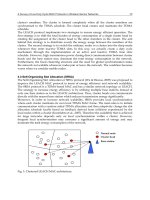
DV-Hop localization algorithm (Niculescu, et al., 2003) was proposed to consider hop counting
for distance estimation. This work uses an approach that is similar to vector routing
algorithms. At first, all sensor nodes broadcast their node ID and information to the nearest
sensor nodes. These surrounding nodes receive it first-hand, thus a distance vector is stored in
these nodes with reference to the source nodes as first hop. These first-hand nodes diffuse
distance vector outward with hop-count values incremented at every intermediate hop. If the
reference nodes receive distance vector with higher hop-count value as compared to
previously received hop-count value, no action is to be taken. As a result, all sensor nodes
have a distance vector of all other sensor nodes. An example of a target node A and the stored
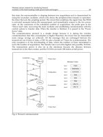
hop-count for the distance vector in all other nodes is shown in Fig. 2 (He, et al., 2005).
Fig. 2. Hop-count Spreading (He, et al., 2005).
After hop-count distances are obtained in every node for all other nodes, the next step of
DV-Hop is to find the average distance between hops using the following expression
(Niculescu, et al., 2003):
j
jiji
i
h
yyxx
HopSize
22
(2)
Emerging Communications for Wireless Sensor Networks234
where HopSize
i
is the average single hop distance for sensor node i. (x
i
, y
i
) is the location of
the node i and (x
j
, y
j
) is the location for all other nodes. h
j
is the hop-count distance from
node j to node i. If the target sensor node can hear more than three sensor nodes which are
location aware, trilateration or multilateration can be used to estimate the location of target
node by combining hop-count distance vector and HopSize.
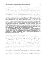
DV-Hop performs well when the deployment of sensor nodes is regular in node density and
the distances among sensor nodes. However, the estimation result may not be optimal if the
radio pattern is irregular and random node deployment is used in practical. To solve this
problem and have better localization result, APIT algorithm (He, et al., 2005) was proposed
for area-based range-free localization solution. In APIT approach, all sensor nodes can be
localized from just few GPS equipped anchors. Using the location information provided
from these anchors, APIT algorithm divides the area occupied by sensor nodes into many
triangular regions among beaconing nodes as shown in Fig. 3 (He, et al., 2005).
Fig. 3. Localization using APIT (He, et al., 2005).
The process of APIT algorithm first starts from localizing sensor nodes using the three GPS
equipped anchors to reduce the possible area that a sensor node may be inside or outside the
triangular regions. After the possible region is reduced, some sensor nodes can be anchors to
further divide the area into more and smaller triangular regions in next round. This process
continues until the possible region of a node can be resided small enough to obtain more
accurate location estimation. This approach provide excellent accuracy when irregular radio
patterns and random node placement are considered, thus it is sufficient to support location
information to various scenarios of applications in sensor networks deployment.
1.2.2 Triangulation Estimation
Triangulation estimation is a trigonometric approach of determining an unknown location
based on two angles and a distance between them. In sensor network, two reference nodes
are required to be located on a horizontal baseline for x axis, and two sensor nodes are
located on a vertical baseline for y axis. The distance d
r
between the two reference nodes on
the baseline can be measured in preliminary stage and stored in memory. The two angles
1
and
2
are measured between the baseline and the line formed by the reference node and
target node as shown in Fig. 4.
Fig. 4. Triangulation Estimation (Pu, 2009).
In Fig. 4, reference nodes R
1
and R
2
form the baseline of X-axis. Reference node R
1
can be
reused to form the baseline of Y-axis together with reference node R
3
. A target node T
1
moves freely around in the area. Based on basic triangulation, the location coordinate (x, y)
of T
1
can be determined by using the combination of R
1
and R
3
to find x, and the
combination of R
1
and R
2
to find y (Pu, 2009):
21
21
21
21
sin
sinsin
sin
sinsin
xx
xxrx
yy
yyry
d
y
d
x
(3)
Alternatively, the expressions can be reformed to a simpler way using trigonometric identity (Pu,
2009):
2
1
1
1
2
1
1
1
tantan
tantan
xx
rx
yy
ry
d
y
d
x
(4)
Depending on the architecture of location system, the computation of triangulation can be
performed either in a centralized system that collects those angle measurements from
distributed reference nodes, or in the target node itself. For the first case, the target node
broadcasts a signal and the surrounding reference nodes measure the angle of received
signal. The reference nodes forward the measured angles to a centralized system as shown
in Fig. 5. In this case, the first reference node measures acute angle and the second node
Indoor Location Tracking using Received Signal Strength Indicator 235
where HopSize
i
is the average single hop distance for sensor node i. (x
i
, y
i
) is the location of
the node i and (x
j
, y
j
) is the location for all other nodes. h
j
is the hop-count distance from
node j to node i. If the target sensor node can hear more than three sensor nodes which are
location aware, trilateration or multilateration can be used to estimate the location of target
node by combining hop-count distance vector and HopSize.
DV-Hop performs well when the deployment of sensor nodes is regular in node density and
the distances among sensor nodes. However, the estimation result may not be optimal if the
radio pattern is irregular and random node deployment is used in practical. To solve this
problem and have better localization result, APIT algorithm (He, et al., 2005) was proposed
for area-based range-free localization solution. In APIT approach, all sensor nodes can be
localized from just few GPS equipped anchors. Using the location information provided
from these anchors, APIT algorithm divides the area occupied by sensor nodes into many
triangular regions among beaconing nodes as shown in Fig. 3 (He, et al., 2005).
Fig. 3. Localization using APIT (He, et al., 2005).
The process of APIT algorithm first starts from localizing sensor nodes using the three GPS
equipped anchors to reduce the possible area that a sensor node may be inside or outside the
triangular regions. After the possible region is reduced, some sensor nodes can be anchors to
further divide the area into more and smaller triangular regions in next round. This process
continues until the possible region of a node can be resided small enough to obtain more
accurate location estimation. This approach provide excellent accuracy when irregular radio
patterns and random node placement are considered, thus it is sufficient to support location
information to various scenarios of applications in sensor networks deployment.
1.2.2 Triangulation Estimation
Triangulation estimation is a trigonometric approach of determining an unknown location
based on two angles and a distance between them. In sensor network, two reference nodes
are required to be located on a horizontal baseline for x axis, and two sensor nodes are
located on a vertical baseline for y axis. The distance d
r
between the two reference nodes on
the baseline can be measured in preliminary stage and stored in memory. The two angles
1
and
2
are measured between the baseline and the line formed by the reference node and
target node as shown in Fig. 4.
Fig. 4. Triangulation Estimation (Pu, 2009).
In Fig. 4, reference nodes R
1
and R
2
form the baseline of X-axis. Reference node R
1
can be
reused to form the baseline of Y-axis together with reference node R
3
. A target node T
1
moves freely around in the area. Based on basic triangulation, the location coordinate (x, y)
of T
1
can be determined by using the combination of R
1
and R
3
to find x, and the
combination of R
1
and R
2
to find y (Pu, 2009):
21
21
21
21
sin
sinsin
sin
sinsin
xx
xxrx
yy
yyry
d
y
d
x
(3)
Alternatively, the expressions can be reformed to a simpler way using trigonometric identity (Pu,
2009):
2
1
1
1
2
1
1
1
tantan
tantan
xx
rx
yy
ry
d
y
d
x
(4)
Depending on the architecture of location system, the computation of triangulation can be
performed either in a centralized system that collects those angle measurements from
distributed reference nodes, or in the target node itself. For the first case, the target node
broadcasts a signal and the surrounding reference nodes measure the angle of received
signal. The reference nodes forward the measured angles to a centralized system as shown
in Fig. 5. In this case, the first reference node measures acute angle and the second node
Emerging Communications for Wireless Sensor Networks236
measures obtuse angle . Thus, the supplementary angle of or ( - ) is the acute angle for
the second node.
Fig. 5. Estimation in Centralized System (Pu, 2009).
For the second case, computation of triangulation can be performed inside the target node if
a magnetic compass is attached to the sensor node. The magnetic compass provides
orientation of the sensor node. All reference nodes broadcast signal to the target node.
Hence, the target node measures the angles , , and from the received signals of the three
reference nodes as shown in Fig. 6. The target sensor node computes its location coordinate
using triangulation and forwards the result to centralized system for data storage or
monitoring purpose.
Fig. 6. Estimation in Target Node (Pu, 2009).
Using electronic magnetic compass (EMC) module attached to the sensor node, an offset
angle can be obtained. This offset angle is used to justify all measurements to a reference
orientation regardless of the sensor node’s orientation. Thus, all acute angles for
triangulation using (3) or (4) can be found as follows (Pu, 2009):
1
2
1
2
0.5
1.5
x
x
y
y
(5)
Besides the mentioned basic triangulation solutions, there are more complicated and complete
solutions using triangulation for different kinds of implementation and environment such as
(Rao, et al., 2007). In addition, the needs of locating objects in three dimensions lead to the
development of dynamic triangulation algorithm (Favre-Bulle, et al., 1998).
Fig. 7. Delaunay Triangulation (Pu, 2009).
With today’s technology, large scale implementation is possible to achieve. Therefore,
localization algorithms also must be good enough for such large scale sensor network
operation. To realize this scenario as shown in Fig. 7, Delaunay triangulation (Li, et al., 2003,
Satyanarayana, et al, 2008) can be used for the localization of multiple points that randomly
forms complicated and connected triangles in the field. The formation of meshed triangles
shape can be optimized using steepest descent method as in (He, 2008). An objective function
was suggested to optimize the shape of triangle elements for the best mesh construction.
1.2.3 Trilateration Estimation
Trilateration estimation is also used to find an unknown location from several reference
locations. However, the difference between trilateration and triangulation is the information
provided into the process of estimation. Instead of measuring the angles among locations,
trilateration uses the distances among the locations to estimate the coordinate of the
unknown location. In trilateration, the distances between reference locations and the
unknown location can be considered as the radii of many circles with centers at every
reference location. Thus, the unknown location is the intersection of all the sphere surfaces
as shown in Fig. 8.
Indoor Location Tracking using Received Signal Strength Indicator 237
measures obtuse angle . Thus, the supplementary angle of or ( - ) is the acute angle for
the second node.
Fig. 5. Estimation in Centralized System (Pu, 2009).
For the second case, computation of triangulation can be performed inside the target node if
a magnetic compass is attached to the sensor node. The magnetic compass provides
orientation of the sensor node. All reference nodes broadcast signal to the target node.
Hence, the target node measures the angles , , and from the received signals of the three
reference nodes as shown in Fig. 6. The target sensor node computes its location coordinate
using triangulation and forwards the result to centralized system for data storage or
monitoring purpose.
Fig. 6. Estimation in Target Node (Pu, 2009).
Using electronic magnetic compass (EMC) module attached to the sensor node, an offset
angle can be obtained. This offset angle is used to justify all measurements to a reference
orientation regardless of the sensor node’s orientation. Thus, all acute angles for
triangulation using (3) or (4) can be found as follows (Pu, 2009):
1
2
1
2
0.5
1.5
x
x
y
y
(5)
Besides the mentioned basic triangulation solutions, there are more complicated and complete
solutions using triangulation for different kinds of implementation and environment such as
(Rao, et al., 2007). In addition, the needs of locating objects in three dimensions lead to the
development of dynamic triangulation algorithm (Favre-Bulle, et al., 1998).
Fig. 7. Delaunay Triangulation (Pu, 2009).
With today’s technology, large scale implementation is possible to achieve. Therefore,
localization algorithms also must be good enough for such large scale sensor network
operation. To realize this scenario as shown in Fig. 7, Delaunay triangulation (Li, et al., 2003,
Satyanarayana, et al, 2008) can be used for the localization of multiple points that randomly
forms complicated and connected triangles in the field. The formation of meshed triangles
shape can be optimized using steepest descent method as in (He, 2008). An objective function
was suggested to optimize the shape of triangle elements for the best mesh construction.
1.2.3 Trilateration Estimation
Trilateration estimation is also used to find an unknown location from several reference
locations. However, the difference between trilateration and triangulation is the information
provided into the process of estimation. Instead of measuring the angles among locations,
trilateration uses the distances among the locations to estimate the coordinate of the
unknown location. In trilateration, the distances between reference locations and the
unknown location can be considered as the radii of many circles with centers at every
reference location. Thus, the unknown location is the intersection of all the sphere surfaces
as shown in Fig. 8.
Emerging Communications for Wireless Sensor Networks238
Fig. 8. Trilateration Estimation (Pu, 2009).
In Fig. 8, three reference nodes are randomly allocated. A target node is moving around the
reference nodes. The target node (T
1
) can be located using the coordinates of the reference
nodes (R
1
, R
2
, and R
3
) and the distances (d
1
, d
2
, d
3
) between the reference nodes and the
target node. A simple solution can be achieved using Pythagorean theorem as shown in the
following expressions (Pu, 2009):
2
3
2
3
2
3
2
2
2
2
2
2
2
1
2
1
2
1
yyxxd
yyxxd
yyxxd
(6)
Rearrange the equations in (6) and solve for x and y, the location coordinate of the target
node can be obtained as shown in the following expressions (Pu, 2009):
213132321
211332
213132321
211332
2
2
XyXyXy
CXBXAX
y
YxYxYx
CYBYAY
x
(7)
where
2
3
2
3
2
3
2
2
2
2
2
2
2
1
2
1
2
1
dyxC
dyxB
dyxA
(8)
and
1221
3113
2332
xxX
xxX
xxX
(9)
1221
3113
2332
yyY
yyY
yyY
(10)
Localization using (7) is very convenient because the distances (d
1
, d
2
, d
3
) can be obtained
from ranging, and the location coordinates of all reference nodes are previously stored in
sensor nodes. In large scale sensor network, perhaps there are only several sensor nodes are
equipped with GPS module. Thus, all other nodes are required to be located using these
GPS equipped sensor nodes.
There are three possible scenarios that localizing a large scale sensor network could meet if
only few sensor nodes among them are equipped with GPS:
1. The sensor nodes are able to reach at least three GPS-node
2. The sensor nodes are able to reach one or two GPS-nodes only
3. The sensor nodes are not able to reach any GPS-node
To use lateration techniques, at least three reference nodes are required. The second and
third scenarios are not able to fulfill the requirement. For this reason, atomic and iterative
multilaterations (Savvides, et al., 2001) were developed for large scale network. Atomic
multilateration is used to estimate the location directly from three or more reference nodes
as shown in Fig. 9(a). If all sensor nodes are able to reach at least three GPS-nodes, then
atomic multilateration is used.
If sensor nodes are too far away from GPS-nodes, it is not able to fulfill the requirement of at
least three reference nodes. Therefore, iterative localization may be considered to spread
location to other nodes. This approach is called iterative multilateration. In this approach,
sensor nodes are converted to reference nodes after localized by GPS-nodes as shown in Fig.
9(b). In next step, these reference nodes can be used to localize other nodes that are not
reachable to GPS-nodes. This process continues until all sensor nodes in the network are
localized.
In a large scale sensor network, atomic and iterative multilaterations can be used to localize
any sensor nodes if the first scenario happens at initial state. However, the random
allocation of GPS-nodes could be far to each other. Thus, no sensor node can reach at least
three GPS-nodes at initial state. This leads to second and third scenarios at initial state. To
solve this problem, collaborative multilateration (Savvides, et al., 2001) was proposed as
shown in Fig. 9(c). In this approach, two sensor nodes are close to each other. These two
sensor nodes are not able to localize themselves as each of them only can reach two GPS-
nodes at initial state. Collaborative multilateration helps to determine their location by
exchanging location information between the two sensor nodes.
Indoor Location Tracking using Received Signal Strength Indicator 239
Fig. 8. Trilateration Estimation (Pu, 2009).
In Fig. 8, three reference nodes are randomly allocated. A target node is moving around the
reference nodes. The target node (T
1
) can be located using the coordinates of the reference
nodes (R
1
, R
2
, and R
3
) and the distances (d
1
, d
2
, d
3
) between the reference nodes and the
target node. A simple solution can be achieved using Pythagorean theorem as shown in the
following expressions (Pu, 2009):
2
3
2
3
2
3
2
2
2
2
2
2
2
1
2
1
2
1
yyxxd
yyxxd
yyxxd
(6)
Rearrange the equations in (6) and solve for x and y, the location coordinate of the target
node can be obtained as shown in the following expressions (Pu, 2009):
213132321
211332
213132321
211332
2
2
XyXyXy
CXBXAX
y
YxYxYx
CYBYAY
x
(7)
where
2
3
2
3
2
3
2
2
2
2
2
2
2
1
2
1
2
1
dyxC
dyxB
dyxA
(8)
and
1221
3113
2332
xxX
xxX
xxX
(9)
1221
3113
2332
yyY
yyY
yyY
(10)
Localization using (7) is very convenient because the distances (d
1
, d
2
, d
3
) can be obtained
from ranging, and the location coordinates of all reference nodes are previously stored in
sensor nodes. In large scale sensor network, perhaps there are only several sensor nodes are
equipped with GPS module. Thus, all other nodes are required to be located using these
GPS equipped sensor nodes.
There are three possible scenarios that localizing a large scale sensor network could meet if
only few sensor nodes among them are equipped with GPS:
1. The sensor nodes are able to reach at least three GPS-node
2. The sensor nodes are able to reach one or two GPS-nodes only
3. The sensor nodes are not able to reach any GPS-node
To use lateration techniques, at least three reference nodes are required. The second and
third scenarios are not able to fulfill the requirement. For this reason, atomic and iterative
multilaterations (Savvides, et al., 2001) were developed for large scale network. Atomic
multilateration is used to estimate the location directly from three or more reference nodes
as shown in Fig. 9(a). If all sensor nodes are able to reach at least three GPS-nodes, then
atomic multilateration is used.
If sensor nodes are too far away from GPS-nodes, it is not able to fulfill the requirement of at
least three reference nodes. Therefore, iterative localization may be considered to spread
location to other nodes. This approach is called iterative multilateration. In this approach,
sensor nodes are converted to reference nodes after localized by GPS-nodes as shown in Fig.
9(b). In next step, these reference nodes can be used to localize other nodes that are not
reachable to GPS-nodes. This process continues until all sensor nodes in the network are
localized.
In a large scale sensor network, atomic and iterative multilaterations can be used to localize
any sensor nodes if the first scenario happens at initial state. However, the random
allocation of GPS-nodes could be far to each other. Thus, no sensor node can reach at least
three GPS-nodes at initial state. This leads to second and third scenarios at initial state. To
solve this problem, collaborative multilateration (Savvides, et al., 2001) was proposed as
shown in Fig. 9(c). In this approach, two sensor nodes are close to each other. These two
sensor nodes are not able to localize themselves as each of them only can reach two GPS-
nodes at initial state. Collaborative multilateration helps to determine their location by
exchanging location information between the two sensor nodes.
Emerging Communications for Wireless Sensor Networks240
Fig. 9. Atomic, Iterative, and Collaborative Multilateration (Savvides, et al., 2001).
2. RSS Ranging in Indoor Environment
2.1 RSS Ranging
The strength of received power from a signal can be used to estimate distance because all
electromagnetic waves have inverse-square relationship between received power and
distance (Savvides, et al., 2001) as shown in the following expression:
2
1
d
P
r
(11)
where P
r
is the received power at a distance d from transmitter. This expression clearly
states that the distance of signal travelled can be found by comparing the difference between
transmission power and received power, or it is called “path loss”.
In practical measurement, the increment of pass loss due to increment of distance may be
different when it is in different environments. This leads to environmental characterization
using path loss exponent n as shown in the following expression (Pu, 2009):
n
d
r
dd
P
p
0
)0(
/
(12)
where P
(d0)
is the received power measured at distance d
0
. Generally, d
0
is fixed as a constant
d
0
= 1 m. Path loss exponent n in the expression is one of the most important parameters for
environmental characterization. If the increment of path loss is more drastic when distance
increases, the value of path loss exponent n would be larger as shown in Fig. 10. The solid
line on top indicates the attenuation or path loss if n = 2.0. The dash line next to the solid
line indicates the attenuation if n = 2.5, and so forth.
Fig. 10. Effects of Path Loss Exponent (Pu, 2009).
Another important feature that constitutes the rules of path loss in Fig. 10 is the beginning
point of each curve. The starting point of all curves is fixed at 37 dBm. If this setting is
smaller, then all curves would be shifted lower. In fact P
(d0)
= 37 dBm exactly. Therefore,
P
(d0)
is also one of the important parameters that characterizes environment
In most radio transceiver modules, the measurement of received power is just an auxiliary
function. The measured value provided by the module may not be exactly received power
in dBm. However, received signal strength indicator (RSSI) is used to represent the
condition of received power level. This can be easily converted to a received power by
applying offset to calibrate to the correct level.
RSSI is generally implemented in most of the wireless communication standards. The
famous standards include IEEE 802.11 and IEEE 802.15.4. RSSI value can be measured in the
intermediate frequency stage, which is before the intermediate frequency amplifier, or in the
baseband stage of circuits. After obtaining RSSI value, the processor or microcontroller with
built-in analog-to-digital converter (ADC) converts it to digital value. This value is then
stored in a register of the controller for quick data acquisition.
2.2 RSSI in Indoor Environment
To use RSS ranging method effectively, we have to identify the differences between indoor
and outdoor location tracking using RSSI. With RSSI adopted, the performance and
implementation methods are totally different between indoor and outdoor. Therefore, if we
Indoor Location Tracking using Received Signal Strength Indicator 241
Fig. 9. Atomic, Iterative, and Collaborative Multilateration (Savvides, et al., 2001).
2. RSS Ranging in Indoor Environment
2.1 RSS Ranging
The strength of received power from a signal can be used to estimate distance because all
electromagnetic waves have inverse-square relationship between received power and
distance (Savvides, et al., 2001) as shown in the following expression:
2
1
d
P
r
(11)
where P
r
is the received power at a distance d from transmitter. This expression clearly
states that the distance of signal travelled can be found by comparing the difference between
transmission power and received power, or it is called “path loss”.
In practical measurement, the increment of pass loss due to increment of distance may be
different when it is in different environments. This leads to environmental characterization
using path loss exponent n as shown in the following expression (Pu, 2009):
n
d
r
dd
P
p
0
)0(
/
(12)
where P
(d0)
is the received power measured at distance d
0
. Generally, d
0
is fixed as a constant
d
0
= 1 m. Path loss exponent n in the expression is one of the most important parameters for
environmental characterization. If the increment of path loss is more drastic when distance
increases, the value of path loss exponent n would be larger as shown in Fig. 10. The solid
line on top indicates the attenuation or path loss if n = 2.0. The dash line next to the solid
line indicates the attenuation if n = 2.5, and so forth.
Fig. 10. Effects of Path Loss Exponent (Pu, 2009).
Another important feature that constitutes the rules of path loss in Fig. 10 is the beginning
point of each curve. The starting point of all curves is fixed at 37 dBm. If this setting is
smaller, then all curves would be shifted lower. In fact P
(d0)
= 37 dBm exactly. Therefore,
P
(d0)
is also one of the important parameters that characterizes environment
In most radio transceiver modules, the measurement of received power is just an auxiliary
function. The measured value provided by the module may not be exactly received power
in dBm. However, received signal strength indicator (RSSI) is used to represent the
condition of received power level. This can be easily converted to a received power by
applying offset to calibrate to the correct level.
RSSI is generally implemented in most of the wireless communication standards. The
famous standards include IEEE 802.11 and IEEE 802.15.4. RSSI value can be measured in the
intermediate frequency stage, which is before the intermediate frequency amplifier, or in the
baseband stage of circuits. After obtaining RSSI value, the processor or microcontroller with
built-in analog-to-digital converter (ADC) converts it to digital value. This value is then
stored in a register of the controller for quick data acquisition.
2.2 RSSI in Indoor Environment
To use RSS ranging method effectively, we have to identify the differences between indoor
and outdoor location tracking using RSSI. With RSSI adopted, the performance and
implementation methods are totally different between indoor and outdoor. Therefore, if we
Emerging Communications for Wireless Sensor Networks242
just consider indoor location tracking scenario, we are able to simplify system complexity
and improve estimation method according to indoor environment.
After going through study and experiments, we considered the differences in design,
implementation, and deployment stages. Table 1 illustrates the comparison between indoor
and outdoor environment.
Outdoor Indoor
Path loss model Linear Affected by multi-path
and shadowing
Accuracy Easy to achieve but not
necessary (wide space)
Difficult to achieve but
important (small space)
Space Wide and not limited Small and mostly
rectangular
Deployment Random and ac hoc Can be planned
Transmission power Maximum to maintain
LQI
Adjusted to avoid
interference
Height of reference
nodes
Ground Ceiling
Map Global Local
Table 1. Comparison of Indoor and Outdoor Location Tracking (Pu, 2009).
In Table 1, path loss model (Phaiboon, 2002) is a radio signal propagation model, which is
used to model the nature of signal attenuation over space. After going through
environmental characterization or calibration, we are able to use this model to convert RSSI
value to distance value.
In indoor environment, the signal strength is not linear as the distance linearly increased
because of multi-path fading (Sklar, 1997) and indoor shadowing (Eltahir, 2007) effects. We
have to study a better way to tackle this problem for better estimation accuracy.
From experiments, we knew that non-linear path loss becomes more serious as the size of
indoor area (for example, a room) is small, leading to difficult accuracy achievement.
However, indoor area is always smaller as compared to outdoor. Thus, the resultant location
error becomes obvious as the accuracy is worst.
To calculate the absolute location coordinate, distances among sensor nodes are combined
using lateration method. When the number of involved reference nodes is increased,
lateration matrix size can be large causing increased computational complexity. Therefore,
we can calculate absolute location coordinate by just using three reference nodes in a room
(trilateration) (Thomas, et al., 2005). This helps to reduce system complexity and
computational power.
In addition, the indoor area is always rectangular shape. During deployment stage, we can
carefully plan the location of various reference nodes. Therefore, ac hoc deployment of
sensor nodes is not suitable to be used in indoor deployment although many researchers
focused on the study of ac hoc sensor network. Through location planning, we can allocate
the reference nodes at strategic locations of the squared area (room). Using this kind of
deployment, we can further simplify estimation formulas. Hence, in-network processing
becomes possible.
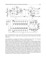
Another important difference between indoor and outdoor implementation is the signal
transmission power. Our experiments show that radio signal energy spread when it
propagates through outdoor free area as shown in Fig. 11. Error! Reference source not
found.This figure indicates the minimum power required to maintain link quality indicator
(LQI) at 100 for various distances. Therefore, transmission power for outdoor environment
must be as high as possible to maintain a safety level of LQI, thus ensuring the quality of
wireless communication channel.
Fig. 11. Minimum Power Required for Communication (Pu, 2009).
On the other hand, signal transmission in indoor environment must be adjusted to suitable
level for interference avoidance from neighbor area. It is not encouraged to use the reference
sensor nodes located in neighbor area to estimate the location coordinate of the target node
in current area. This is because path loss model could be seriously inaccurate and non-linear
while radio signal propagates through wall with high signal attenuation. There is no worry
about maintaining LQI as difficult as outdoor because the radio signal energy can be
conserved within enclosed area.
For outdoor ac hoc deployment, sensor nodes are allocated randomly on ground. However,
indoor deployment requires the reference nodes to be fixed beneath ceiling to avoid
obstacles and must be the same height among them. This manual installation of reference
nodes also needs to be planed for better strategic location. Because of the partitioned area of
indoor space, it is more convenient if we display the target node’s location using local axis
method. In this method, every area has its own axis. To find location in the display map,
areas can be differentiated by area ID.
3. Location Tracking System Design and Implementation
The design of a complete location system involves three areas of knowledge including (a)
the signal and information processing to compute location information as output, (b)
Indoor Location Tracking using Received Signal Strength Indicator 243
just consider indoor location tracking scenario, we are able to simplify system complexity
and improve estimation method according to indoor environment.
After going through study and experiments, we considered the differences in design,
implementation, and deployment stages. Table 1 illustrates the comparison between indoor
and outdoor environment.
Outdoor Indoor
Path loss model Linear Affected by multi-path
and shadowing
Accuracy Easy to achieve but not
necessary (wide space)
Difficult to achieve but
important (small space)
Space Wide and not limited Small and mostly
rectangular
Deployment Random and ac hoc Can be planned
Transmission power Maximum to maintain
LQI
Adjusted to avoid
interference
Height of reference
nodes
Ground Ceiling
Map Global Local
Table 1. Comparison of Indoor and Outdoor Location Tracking (Pu, 2009).
In Table 1, path loss model (Phaiboon, 2002) is a radio signal propagation model, which is
used to model the nature of signal attenuation over space. After going through
environmental characterization or calibration, we are able to use this model to convert RSSI
value to distance value.
In indoor environment, the signal strength is not linear as the distance linearly increased
because of multi-path fading (Sklar, 1997) and indoor shadowing (Eltahir, 2007) effects. We
have to study a better way to tackle this problem for better estimation accuracy.
From experiments, we knew that non-linear path loss becomes more serious as the size of
indoor area (for example, a room) is small, leading to difficult accuracy achievement.
However, indoor area is always smaller as compared to outdoor. Thus, the resultant location
error becomes obvious as the accuracy is worst.
To calculate the absolute location coordinate, distances among sensor nodes are combined
using lateration method. When the number of involved reference nodes is increased,
lateration matrix size can be large causing increased computational complexity. Therefore,
we can calculate absolute location coordinate by just using three reference nodes in a room
(trilateration) (Thomas, et al., 2005). This helps to reduce system complexity and
computational power.
In addition, the indoor area is always rectangular shape. During deployment stage, we can
carefully plan the location of various reference nodes. Therefore, ac hoc deployment of
sensor nodes is not suitable to be used in indoor deployment although many researchers
focused on the study of ac hoc sensor network. Through location planning, we can allocate
the reference nodes at strategic locations of the squared area (room). Using this kind of
deployment, we can further simplify estimation formulas. Hence, in-network processing
becomes possible.
Another important difference between indoor and outdoor implementation is the signal
transmission power. Our experiments show that radio signal energy spread when it
propagates through outdoor free area as shown in Fig. 11. Error! Reference source not
found.This figure indicates the minimum power required to maintain link quality indicator
(LQI) at 100 for various distances. Therefore, transmission power for outdoor environment
must be as high as possible to maintain a safety level of LQI, thus ensuring the quality of
wireless communication channel.
Fig. 11. Minimum Power Required for Communication (Pu, 2009).
On the other hand, signal transmission in indoor environment must be adjusted to suitable
level for interference avoidance from neighbor area. It is not encouraged to use the reference
sensor nodes located in neighbor area to estimate the location coordinate of the target node
in current area. This is because path loss model could be seriously inaccurate and non-linear
while radio signal propagates through wall with high signal attenuation. There is no worry
about maintaining LQI as difficult as outdoor because the radio signal energy can be
conserved within enclosed area.
For outdoor ac hoc deployment, sensor nodes are allocated randomly on ground. However,
indoor deployment requires the reference nodes to be fixed beneath ceiling to avoid
obstacles and must be the same height among them. This manual installation of reference
nodes also needs to be planed for better strategic location. Because of the partitioned area of
indoor space, it is more convenient if we display the target node’s location using local axis
method. In this method, every area has its own axis. To find location in the display map,
areas can be differentiated by area ID.
3. Location Tracking System Design and Implementation
The design of a complete location system involves three areas of knowledge including (a)
the signal and information processing to compute location information as output, (b)
Emerging Communications for Wireless Sensor Networks244
realization of the system by implementing using various technologies available, and (c)
acquisition of location data and store, analyze, monitor, and display in a centralized
management server. In this chapter, the first two areas are the focus whereas the third area
was excluded.
3.1 System Design
In general, the first task to be considered in a location system design work is the core of
information handling through signal processing and data mining. This decides how the
process goes through from raw signal to valuable information.
3.1.1 System Block Diagram
We need to consider how to find the location coordinate from raw RSSI data. It has to go
through several processing steps as shown in Fig. 12.
Fig. 12. The Findings of Location from Raw RSSI (Pu, 2009).
In Fig. 12, RSSI values are collected from reference nodes in distance estimation step. Using
these RSSI values, we can perform environmental characterization to find suitable
parameters for that area. When calibration process is over, the environmental parameters
are fixed and will not be change unless large changes happen to the objects within the area.
The next step is to obtain continuous RSSI values from the reference nodes in the online
operation. With both RSSI values and environmental parameters ready, we can convert
those RSSI values into distance using path loss model.
After RSSI-Distance conversion, we are able to obtain the distances between target sensor
node and the reference nodes. By applying trilateration, it combines distances and find the
exact location coordinate of the target sensor node within the area. The overall system block
diagram is shown in Fig. 13.
Fig. 13. Overall System Block Diagram (Pu, 2009).
3.1.2 RSSI Measurement Step
In this step, RSSI values are collected from the reference sensor nodes. Practically, RSSI
value is not exactly the received power at the RF pins of the radio transceiver. Therefore, it
has to be converted to the actual power values in dBm using the following expression (Pu,
2009):
offset
RSSIRSSIP
ii
(13)
where P
i
is the actual received power from beacon node i. RSSI
i
is the measured RSSI value
for reference node i, which is stored in the RSSI register of the radio transceiver. RSSI
offset
is
the offset found empirically from the front end gain and it is approximately equal to 45
dBm. This is to make sure that the actual received power value has dynamic range from
100 to 0 dBm, where 100 dBm indicates the minimum power that can receive, and 0 dBm
indicates the maximum received power.
3.1.3 RSSI Signal Improvement Step
In indoor environment, raw RSSI data is highly uncertain and it is fluctuating over time. The
study must go back to the investigation of radio signal propagation in indoor environment.
For RSS ranging application, the analysis of the radio propagation manner is slightly
different from the well-established theory for just digital communication purpose.
In digital communication, the study of received power is to avoid burst error and ensure
high bit-error rate communication. The level change of RSS is not important as long as it is
maintained within the safety region. However, when RSS is used in estimating distance, the
estimation result is directly based on the level of RSS. Therefore, it is necessary to improve
the signal quality of RSS.
From analysis, the reasons of RSSI variation in indoor environment can be well categorized
for better understanding as shown in Fig. 14. Based on past research and analysis, we
classified the reasons of RSSI variation in terms of both small/large scale and
temporal/spatial characteristics. Fig. 14 clearly states all possible reasons of indoor RSSI
variation in the two-dimensional classification diagram. In term of scale level, RSSI variation
can be fluctuating slowly or quickly if it is in the temporal domain, and fluctuating narrowly
or widely if it is in the spatial domain.
Indoor Location Tracking using Received Signal Strength Indicator 245
realization of the system by implementing using various technologies available, and (c)
acquisition of location data and store, analyze, monitor, and display in a centralized
management server. In this chapter, the first two areas are the focus whereas the third area
was excluded.
3.1 System Design
In general, the first task to be considered in a location system design work is the core of
information handling through signal processing and data mining. This decides how the
process goes through from raw signal to valuable information.
3.1.1 System Block Diagram
We need to consider how to find the location coordinate from raw RSSI data. It has to go
through several processing steps as shown in Fig. 12.
Fig. 12. The Findings of Location from Raw RSSI (Pu, 2009).
In Fig. 12, RSSI values are collected from reference nodes in distance estimation step. Using
these RSSI values, we can perform environmental characterization to find suitable
parameters for that area. When calibration process is over, the environmental parameters
are fixed and will not be change unless large changes happen to the objects within the area.
The next step is to obtain continuous RSSI values from the reference nodes in the online
operation. With both RSSI values and environmental parameters ready, we can convert
those RSSI values into distance using path loss model.
After RSSI-Distance conversion, we are able to obtain the distances between target sensor
node and the reference nodes. By applying trilateration, it combines distances and find the
exact location coordinate of the target sensor node within the area. The overall system block
diagram is shown in Fig. 13.
Fig. 13. Overall System Block Diagram (Pu, 2009).
3.1.2 RSSI Measurement Step
In this step, RSSI values are collected from the reference sensor nodes. Practically, RSSI
value is not exactly the received power at the RF pins of the radio transceiver. Therefore, it
has to be converted to the actual power values in dBm using the following expression (Pu,
2009):
offset
RSSIRSSIP
ii
(13)
where P
i
is the actual received power from beacon node i. RSSI
i
is the measured RSSI value
for reference node i, which is stored in the RSSI register of the radio transceiver. RSSI
offset
is
the offset found empirically from the front end gain and it is approximately equal to 45
dBm. This is to make sure that the actual received power value has dynamic range from
100 to 0 dBm, where 100 dBm indicates the minimum power that can receive, and 0 dBm
indicates the maximum received power.
3.1.3 RSSI Signal Improvement Step
In indoor environment, raw RSSI data is highly uncertain and it is fluctuating over time. The
study must go back to the investigation of radio signal propagation in indoor environment.
For RSS ranging application, the analysis of the radio propagation manner is slightly
different from the well-established theory for just digital communication purpose.
In digital communication, the study of received power is to avoid burst error and ensure
high bit-error rate communication. The level change of RSS is not important as long as it is
maintained within the safety region. However, when RSS is used in estimating distance, the
estimation result is directly based on the level of RSS. Therefore, it is necessary to improve
the signal quality of RSS.
From analysis, the reasons of RSSI variation in indoor environment can be well categorized
for better understanding as shown in Fig. 14. Based on past research and analysis, we
classified the reasons of RSSI variation in terms of both small/large scale and
temporal/spatial characteristics. Fig. 14 clearly states all possible reasons of indoor RSSI
variation in the two-dimensional classification diagram. In term of scale level, RSSI variation
can be fluctuating slowly or quickly if it is in the temporal domain, and fluctuating narrowly
or widely if it is in the spatial domain.
Emerging Communications for Wireless Sensor Networks246
Fig. 14. Types of RSSI Variation in Indoor Environment (Pu, 2009).
Fast fading belongs to small scale variation such as multipath or Rayleigh fading, and
environmental changes belongs to large scale variation as it is slowly time-variant. In the
spatial domain, RSSI values do not vary in the stationary condition. RSSI values vary only
when receiver moves over space or distance. Multipath or Rayleigh fading is also a spatial
small scale variation. Log-distance path loss model is a large scale effect in spatial domain.
Lognormal shadowing is considered as a medium size variation in the space domain.
To improve RSSI signal from both temporal and spatial variation, we can use a modified
version of Kalman filter that estimates the speed of variation and use it to predict the future
possible values. Based on past, current and future predicted values, RSSI variation can be
reduced. With this, it is also able to cover some parts of small and large scale variation. The
update of current RSSI and its variation speed can be found using the following expressions
(Pu, 2009):
ipredipreviprediest
RRaRR
ˆˆˆ
(14)
iprediprev
s
iprediest
RR
T
b
VV
ˆˆˆ
(15)
The prediction of the RSSI and its variation speed can be found using the following
expressions (Pu, 2009):
siestiestipred
TVRR
ˆˆˆ
1
(16)
iestipred
VV
ˆˆ
1
(17)
where
iest
R
ˆ
is the i
th
estimation value of RSSI,
ipred
R
ˆ
is the i
th
predicted value of RSSI,
iprev
R is the i
th
previous value of RSSI,
iest
V
ˆ
and
ipred
V
ˆ
are the i
th
estimation speed
and i
th
predicted speed. Parameters a and b are the gain constant, T
s
is the time duration of
samples arrival. After going through this processing, highly fluctuating RSSI values are
smoothed and become more stable.
3.1.4 Environmental Characterization Step
In this step, RSSI values are collected with the corresponding location of target node. Using
the pair of (RSSI, Location) information to calibrate system parameters to the most
appropriate level. After environmental characterization step, the distance estimation of the
signal is adjusted to the minimum error state.
The important parameters used to characterize environment include path loss exponent n
and the received power P
r(d0)
measured at distance d
0
to the transmitter. For each enclosed
area of indoor environment, a pair of these parameters (n, P
r(d0)
) are used to represent the
conditions of the area. To characterize the area for RSS ranging, received power P
r(d0)
is first
measured by allocating a receiver d
0
apart from the transmitter. d
0
is generally fixed at 1
meter. After P
r(d0)
is obtained, the receiver is moved to other locations to measure path loss
exponent n using the following expression (Pu, 2009):
010
)()0(
/log10 dd
PP
n
drdr
(18)
where P
r(d)
is the received power of the receiver measured at a distance d to the transmitter,
which is expressed in dBm.
Theoretically, every room or area has their environmental parameters. However, the fact is
that every location also has their environmental parameters although two locations are in
the same room and they are neighbor. The reasons of this problem are from the RSSI
variation in indoor environment especially in the medium scale spatial domain variation.
Suppose we use inaccurate and uncertain RSSI source for calibration, it is impossible that we
are able to obtain accurate environmental parameters from experiments. There will be
different environmental parameters obtain at every location. This indeed increases the
difficulty of environmental calibration works.
3.1.5 RSSI-Distance Conversion Step
If RSS ranging is used to measure the distances between reference nodes and target node,
log-distance path loss model (Phaiboon, 2002) is used to express the relationship between
received power and the corresponding distance as shown in the following expression (Pu,
2009):
0
10)0()(
log10
d
d
nPP
drdr
(19)
After the step of environmental characterization, the two main environmental parameters n
and P
r(d0)
are obtained. Thus, the distance between transmitter and receiver can be estimated
using the following expression (Pu, 2009):
( 0) ( )
0
exp
10
r d r d
P P
d d
n
(20)
Indoor Location Tracking using Received Signal Strength Indicator 247
Fig. 14. Types of RSSI Variation in Indoor Environment (Pu, 2009).
Fast fading belongs to small scale variation such as multipath or Rayleigh fading, and
environmental changes belongs to large scale variation as it is slowly time-variant. In the
spatial domain, RSSI values do not vary in the stationary condition. RSSI values vary only
when receiver moves over space or distance. Multipath or Rayleigh fading is also a spatial
small scale variation. Log-distance path loss model is a large scale effect in spatial domain.
Lognormal shadowing is considered as a medium size variation in the space domain.
To improve RSSI signal from both temporal and spatial variation, we can use a modified
version of Kalman filter that estimates the speed of variation and use it to predict the future
possible values. Based on past, current and future predicted values, RSSI variation can be
reduced. With this, it is also able to cover some parts of small and large scale variation. The
update of current RSSI and its variation speed can be found using the following expressions
(Pu, 2009):
ipredipreviprediest
RRaRR
ˆˆˆ
(14)
iprediprev
s
iprediest
RR
T
b
VV
ˆˆˆ
(15)
The prediction of the RSSI and its variation speed can be found using the following
expressions (Pu, 2009):
siestiestipred
TVRR
ˆˆˆ
1
(16)
iestipred
VV
ˆˆ
1
(17)
where
iest
R
ˆ
is the i
th
estimation value of RSSI,
ipred
R
ˆ
is the i
th
predicted value of RSSI,
iprev
R is the i
th
previous value of RSSI,
iest
V
ˆ
and
ipred
V
ˆ
are the i
th
estimation speed
and i
th
predicted speed. Parameters a and b are the gain constant, T
s
is the time duration of
samples arrival. After going through this processing, highly fluctuating RSSI values are
smoothed and become more stable.
3.1.4 Environmental Characterization Step
In this step, RSSI values are collected with the corresponding location of target node. Using
the pair of (RSSI, Location) information to calibrate system parameters to the most
appropriate level. After environmental characterization step, the distance estimation of the
signal is adjusted to the minimum error state.
The important parameters used to characterize environment include path loss exponent n
and the received power P
r(d0)
measured at distance d
0
to the transmitter. For each enclosed
area of indoor environment, a pair of these parameters (n, P
r(d0)
) are used to represent the
conditions of the area. To characterize the area for RSS ranging, received power P
r(d0)
is first
measured by allocating a receiver d
0
apart from the transmitter. d
0
is generally fixed at 1
meter. After P
r(d0)
is obtained, the receiver is moved to other locations to measure path loss
exponent n using the following expression (Pu, 2009):
010
)()0(
/log10 dd
PP
n
drdr
(18)
where P
r(d)
is the received power of the receiver measured at a distance d to the transmitter,
which is expressed in dBm.
Theoretically, every room or area has their environmental parameters. However, the fact is
that every location also has their environmental parameters although two locations are in
the same room and they are neighbor. The reasons of this problem are from the RSSI
variation in indoor environment especially in the medium scale spatial domain variation.
Suppose we use inaccurate and uncertain RSSI source for calibration, it is impossible that we
are able to obtain accurate environmental parameters from experiments. There will be
different environmental parameters obtain at every location. This indeed increases the
difficulty of environmental calibration works.
3.1.5 RSSI-Distance Conversion Step
If RSS ranging is used to measure the distances between reference nodes and target node,
log-distance path loss model (Phaiboon, 2002) is used to express the relationship between
received power and the corresponding distance as shown in the following expression (Pu,
2009):
0
10)0()(
log10
d
d
nPP
drdr
(19)
After the step of environmental characterization, the two main environmental parameters n
and P
r(d0)
are obtained. Thus, the distance between transmitter and receiver can be estimated
using the following expression (Pu, 2009):
( 0) ( )
0
exp
10
r d r d
P P
d d
n
(20)
Emerging Communications for Wireless Sensor Networks248
In this expression, the estimated distance d is in centimeter if the value of d
0
provided is in
centimeter such as d
0
= 100 cm.
3.1.6 Trilateration Step
In indoor environment, the shapes of target area are in arbitrary shape. The location
coordinate of the target node can be estimated using trilateration by applying equation (7).
Nevertheless, we are able to implement the reference nodes of location system in a regular
way such as in a shape of rectangle or square. This helps to reduce the computation
complexity of lateration. Two approaches of strategic reference node allocation can be
considered as shown in Fig. 15. Error! Reference source not found.
Fig. 15. Locations for Simplified Trilateration (Pu, 2009).
In Fig. 15(a), the reference sensor nodes are located at the corners of the rectangular area.
This approach only requires three reference nodes for trilateration. To estimate the location
coordinate, two reference sensor nodes R1 and R2 along the x-axis are sufficient to provide
inputs for calculating x. Since reference node R1 is aligned with R3 along the y-axis, R1 also
can be used together with R3 to provide inputs for calculating y.
In Fig. 15(b), the reference sensor nodes are located at the edges of the rectangular area. This
approach requires four reference nodes for trilateration. To estimate the location coordinate
of target node, two reference nodes R1 and R2 are used to provide inputs for calculating x
while R3 and R4 are used to provide inputs for calculating y.
The distances among sensor nodes (d
1
, d
2
, d
3
, and d
4
) are obtained using log-distance path
loss model to convert RSSI values to distances. The distances (d
1
and d
2
) can be used to
determine x as shown in the following expression (Pu, 2009):
u
ddu
x
2
2
2
2
1
2
(21)
In the first approach, the distances (d
1
and d
3
) can be used to determine y as shown in the
following expression (Pu, 2009):
v
ddv
y
2
2
3
2
1
2
(22)
In the second approach, the distances (d
3
and d
4
) can be used to determine y as shown in the
following expression (Pu, 2009):
v
ddv
y
2
2
4
2
3
2
(23)
3.2 Network Implementation
After the flow of location information processing was decided, the next step is to investigate
the current technologies available and choose the most suitable solution to implement the
operation network. Among many alternatives, WSN technology has the capability to
perform such indoor location system works and it provides many advantages for ubiquitous
implementation.
These advantages include: low power consumption, devices are not expensive, small size,
software configurable and flexible, wide radio coverage, good processing ability, sufficient
I/O for sensing and actuating, and etc. Most important factor is that WSN has been well
established in various fields of research. Therefore, many resources and good algorithms are
available from other research efforts. Hence, WSN was chosen as the main operation
network to implement indoor location system.
3.2.1 Network Structure
The construction of the operation network for indoor location system based on WSN is
related to the source of raw data and the sink of useful information. Thus, the characteristics
of the WSN implementation for indoor location system are investigated and shown in Fig.
16 and the following points:
Fig. 16. Network Structure (Pu, 2009).
Indoor Location Tracking using Received Signal Strength Indicator 249
In this expression, the estimated distance d is in centimeter if the value of d
0
provided is in
centimeter such as d
0
= 100 cm.
3.1.6 Trilateration Step
In indoor environment, the shapes of target area are in arbitrary shape. The location
coordinate of the target node can be estimated using trilateration by applying equation (7).
Nevertheless, we are able to implement the reference nodes of location system in a regular
way such as in a shape of rectangle or square. This helps to reduce the computation
complexity of lateration. Two approaches of strategic reference node allocation can be
considered as shown in Fig. 15. Error! Reference source not found.
Fig. 15. Locations for Simplified Trilateration (Pu, 2009).
In Fig. 15(a), the reference sensor nodes are located at the corners of the rectangular area.
This approach only requires three reference nodes for trilateration. To estimate the location
coordinate, two reference sensor nodes R1 and R2 along the x-axis are sufficient to provide
inputs for calculating x. Since reference node R1 is aligned with R3 along the y-axis, R1 also
can be used together with R3 to provide inputs for calculating y.
In Fig. 15(b), the reference sensor nodes are located at the edges of the rectangular area. This
approach requires four reference nodes for trilateration. To estimate the location coordinate
of target node, two reference nodes R1 and R2 are used to provide inputs for calculating x
while R3 and R4 are used to provide inputs for calculating y.
The distances among sensor nodes (d
1
, d
2
, d
3
, and d
4
) are obtained using log-distance path
loss model to convert RSSI values to distances. The distances (d
1
and d
2
) can be used to
determine x as shown in the following expression (Pu, 2009):
u
ddu
x
2
2
2
2
1
2
(21)
In the first approach, the distances (d
1
and d
3
) can be used to determine y as shown in the
following expression (Pu, 2009):
v
ddv
y
2
2
3
2
1
2
(22)
In the second approach, the distances (d
3
and d
4
) can be used to determine y as shown in the
following expression (Pu, 2009):
v
ddv
y
2
2
4
2
3
2
(23)
3.2 Network Implementation
After the flow of location information processing was decided, the next step is to investigate
the current technologies available and choose the most suitable solution to implement the
operation network. Among many alternatives, WSN technology has the capability to
perform such indoor location system works and it provides many advantages for ubiquitous
implementation.
These advantages include: low power consumption, devices are not expensive, small size,
software configurable and flexible, wide radio coverage, good processing ability, sufficient
I/O for sensing and actuating, and etc. Most important factor is that WSN has been well
established in various fields of research. Therefore, many resources and good algorithms are
available from other research efforts. Hence, WSN was chosen as the main operation
network to implement indoor location system.
3.2.1 Network Structure
The construction of the operation network for indoor location system based on WSN is
related to the source of raw data and the sink of useful information. Thus, the characteristics
of the WSN implementation for indoor location system are investigated and shown in Fig.
16 and the following points:
Fig. 16. Network Structure (Pu, 2009).
Emerging Communications for Wireless Sensor Networks250
1. Network is constructed to support monitoring all the time, thus all sources of
information send data constantly to a base station.
2. The network is multi-source single sink data network.
3. The data direction is from source to sink, thus no query service is available.
4. According to the movement status of sensor nodes, there are two types of network
nodes: stationary and mobile nodes
5. All sensor nodes including stationary and mobile nodes can be an intermediate node
for routing packets to base station.
6. The sensor nodes located in the same indoor area can be organized together as a
cluster of the network.
7. A cluster consists of both stationary and mobile nodes. Cluster with only stationary
nodes is possible but cluster with pure mobile nodes does not exist.
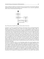
3.2.2 Interaction and Scheduling
For network implementation, communication signals are initiated from mobile nodes. This
is to make sure that when mobile node enters a new zone, it is able to wake up all reference
nodes. When a reference node cannot hear any mobile node for more than ten seconds, the
reference node will be automatically switched to inactive mode. To save power
consumption, an accelerometer can be installed into the sensor node. Whenever there is
motion, the accelerometer is able to activate mobile node, and the mobile node activates
other reference nodes. The communication paths are shown in Fig. 17.
Fig. 17. Interaction and Communication Paths (Pu, 2009).
For communication path (i), target node T2 broadcasts a message to all reference nodes (R1,
R3, R5). Reference nodes are awaked and reply to T2 with (ii). T2 then collects the IDs and
RSSI values from all reference nodes and estimate location coordinate of the target node.
The resultant location information is then forwarded to base station (B0) through path (iii).
Base station forwards the data to a computer through USB (iv) for display and monitoring.
To save power consumption and last the life of batteries in the sensor nodes, reference nodes
are in inactive mode when there is no target node in the area. When a target node moves
into the area, the movement of the target node causes motion sensor to generate activation
signal. The activation signal is broadcasted to activate all reference nodes in the area.
A problem exists in this interaction among sensor nodes. When the number of reference
nodes is increased, the problem becomes more serious. This problem arises because all
reference nodes receive the activation signal from target node at the same time. In this case,
all reference nodes are synchronized and send estimation signal for RSS ranging at the same
time. Therefore, the target node receives all the estimation signals to measure RSSI at the
same time. Inevitably, packet loss happens, leading to operation failure.
To solve this problem, transmission scheduling must be considered in the reference nodes.
There are three kinds of transmission scheduling can be considered in indoor location
tracking system implementation:
1. Use a random number generator to produce time delay t
d
for the first estimation
signal. The duration of delay can be obtained using the random number n
r
(ranged
from 0 to 1) as shown in the following expression (Pu, 2009):
rd
nTt
(24)
2. Use a fixed number n
id
obtained from the node ID or address to produce time delay t
d
for the first estimation signal. The duration of delay can be obtained using the
following expression (Pu, 2009):
N
n
Tt
id
d
(25)
3. Use a fixed number n
g
obtained from the group ID to produce time delay t
d
for the
first estimation signal. Group ID is used to differentiate the sensor nodes within the
same indoor area or cluster assigned by cluster head. Thus, the duration of delay can
be obtained using the following expression (Pu, 2009):
G
n
Tt
g
d
(26)
where T represents the transmission period of the estimation signal broadcasted from
reference nodes, N is the total number of sensor nodes used in the indoor location system
network, and G is the total number of member nodes in a cluster.
The first kind of transmission scheduling may still have signal collision problem as two
reference nodes generate the same random number. However, the advantage is the ease of
implementation. The second kind of transmission scheduling may have problem when the
number of total sensor nodes is large and the transmission period T is short. This causes the
divided delay time duration too short. In addition, expansion of network increases the total
number of nodes, leading to unnecessary reinstallation to all sensor nodes. The third kind of
transmission scheduling is a good choice, but it depends on the good clustering result of
network.
3.2.3 In-network Processing
Wireless sensor network is formed by spatially distributed wireless sensor motes that are
able to work independently or cooperatively with other sensor motes. Due to the size
Indoor Location Tracking using Received Signal Strength Indicator 251
1. Network is constructed to support monitoring all the time, thus all sources of
information send data constantly to a base station.
2. The network is multi-source single sink data network.
3. The data direction is from source to sink, thus no query service is available.
4. According to the movement status of sensor nodes, there are two types of network
nodes: stationary and mobile nodes
5. All sensor nodes including stationary and mobile nodes can be an intermediate node
for routing packets to base station.
6. The sensor nodes located in the same indoor area can be organized together as a
cluster of the network.
7. A cluster consists of both stationary and mobile nodes. Cluster with only stationary
nodes is possible but cluster with pure mobile nodes does not exist.
3.2.2 Interaction and Scheduling
For network implementation, communication signals are initiated from mobile nodes. This
is to make sure that when mobile node enters a new zone, it is able to wake up all reference
nodes. When a reference node cannot hear any mobile node for more than ten seconds, the
reference node will be automatically switched to inactive mode. To save power
consumption, an accelerometer can be installed into the sensor node. Whenever there is
motion, the accelerometer is able to activate mobile node, and the mobile node activates
other reference nodes. The communication paths are shown in Fig. 17.
Fig. 17. Interaction and Communication Paths (Pu, 2009).
For communication path (i), target node T2 broadcasts a message to all reference nodes (R1,
R3, R5). Reference nodes are awaked and reply to T2 with (ii). T2 then collects the IDs and
RSSI values from all reference nodes and estimate location coordinate of the target node.
The resultant location information is then forwarded to base station (B0) through path (iii).
Base station forwards the data to a computer through USB (iv) for display and monitoring.
To save power consumption and last the life of batteries in the sensor nodes, reference nodes
are in inactive mode when there is no target node in the area. When a target node moves
into the area, the movement of the target node causes motion sensor to generate activation
signal. The activation signal is broadcasted to activate all reference nodes in the area.
A problem exists in this interaction among sensor nodes. When the number of reference
nodes is increased, the problem becomes more serious. This problem arises because all
reference nodes receive the activation signal from target node at the same time. In this case,
all reference nodes are synchronized and send estimation signal for RSS ranging at the same
time. Therefore, the target node receives all the estimation signals to measure RSSI at the
same time. Inevitably, packet loss happens, leading to operation failure.
To solve this problem, transmission scheduling must be considered in the reference nodes.
There are three kinds of transmission scheduling can be considered in indoor location
tracking system implementation:
1. Use a random number generator to produce time delay t
d
for the first estimation
signal. The duration of delay can be obtained using the random number n
r
(ranged
from 0 to 1) as shown in the following expression (Pu, 2009):
rd
nTt
(24)
2. Use a fixed number n
id
obtained from the node ID or address to produce time delay t
d
for the first estimation signal. The duration of delay can be obtained using the
following expression (Pu, 2009):
N
n
Tt
id
d
(25)
3. Use a fixed number n
g
obtained from the group ID to produce time delay t
d
for the
first estimation signal. Group ID is used to differentiate the sensor nodes within the
same indoor area or cluster assigned by cluster head. Thus, the duration of delay can
be obtained using the following expression (Pu, 2009):
G
n
Tt
g
d
(26)
where T represents the transmission period of the estimation signal broadcasted from
reference nodes, N is the total number of sensor nodes used in the indoor location system
network, and G is the total number of member nodes in a cluster.
The first kind of transmission scheduling may still have signal collision problem as two
reference nodes generate the same random number. However, the advantage is the ease of
implementation. The second kind of transmission scheduling may have problem when the
number of total sensor nodes is large and the transmission period T is short. This causes the
divided delay time duration too short. In addition, expansion of network increases the total
number of nodes, leading to unnecessary reinstallation to all sensor nodes. The third kind of
transmission scheduling is a good choice, but it depends on the good clustering result of
network.
3.2.3 In-network Processing
Wireless sensor network is formed by spatially distributed wireless sensor motes that are
able to work independently or cooperatively with other sensor motes. Due to the size
Emerging Communications for Wireless Sensor Networks252
constraint, the individual device in wireless sensor network is normally limited in
processing capability, storage capacity, communication bandwidth, and battery power
supply (Culler, et al., 2004). The battery life-time and the communication bandwidth usage
are generally treated higher priority than the rest since in most applications, battery may not
be frequently recharged or replaced. Saving bandwidth or reducing the data transmission
among sensor nodes also means reducing power consumption used in communication.
Therefore, various algorithms such as collaborative signal processing, adaptive system,
distributed algorithm, and sensor fusion were developed for low power and bandwidth
applications.
Recently, a new trend of study is focused on in-network processing and intelligent system
such as (Tseng, et al., 2007) and (Yang, et al., 2007). For the applications of location tracking,
(Liu, et al., 2003) develop the initial concept of collaborative in-network processing for target
tracking. The focus is on vehicle tracking using acoustic and direction-of-arrival sensors.
(Lin, et al., 2004, 2006) presents in-network moving object tracking. The way of tracking
object is based on detection in a mass deployment of sensor nodes.
In general, the received RSSI values from reference nodes are sent to base station
immediately. The based station is an interface between WSN and computer, which collects
sufficient RSSI values and forwards them to the computer. In this case, location estimation
task is performed and stored in the computer.
Besides the monitoring of user’s activities, location information also can be used to support
the needs of network routing, data sensing, information query, self-organization, task
scheduling, field coverage, and etc. If the sensor nodes need the resultant location
information for decision making, the computer has to send the computed location
estimation result back to sensor nodes through the network. In this way, location estimation
does not consume processing power in the sensor nodes but this greatly increases the
wireless data transmission traffic for multi-user condition.
For a compromise, it is better to let the sensor nodes to collect all RSSI values and estimate
location coordinates locally within the WSN. The estimated location information is then
forwarded to a computer for monitoring or display. This approach also provides fast
location update rate due to short packets used. If the location information can be updated
immediately, the response and operation sensing tasks can be active, and the time taken for
decision making is short. The architectures of estimating location coordinate in a computer
and in sensor nodes are shown in Fig. 18.
Fig. 18. Two Scenarios of Location Estimation (Pu, 2009).
In Fig. 18(a), R1 to R3 are reference nodes in the area. A mobile node L1 is hold by a user
and moving around the area. L1 collects data from all reference nodes, and forwards them
to a computer. The packet includes the ID of each reference nodes (ID
R1
, ID
R2
, ID
R3
,), RSSI
values from each reference node (RSSI
1
, RSSI
2
, RSSI
3
,), and the ID of the mobile node (ID
L1
).
If the number of reference node increases, the packet size would be large. This largely
increases network traffic and load.
In Fig. 18 (b), R4 to R6 are reference nodes in the area. A mobile node L2 is hold by user and
moving around the area. L2 collects data from all reference nodes, and perform location
estimation locally. The resultant packet is then forwarded to computer. Hence, the packet
only includes the coordinate (x, y), space ID (SP
01
), and the ID of the mobile node (ID
L2
). If
the number of reference node increases, the packet size does not increase but still remains
small and constant because only the estimation result is forwarded to computer.
Wireless sensor network have substantial processing capability in the aggregate, but not
individually. For most of the low-power mobile device such as wireless sensor motes, the
processors or microcontrollers are limited in computational capability. For this reason,
indoor location estimation algorithms must be simple and ease of implementation.
For ensuring light-weight processing and tool-independent programming, it is necessary to
consider carefully that algorithms, mathematical calculations and processing are simple and
programmable to any low-power mobile devices which have limitation and constraints. The
main computational loads are in RSSI-distance conversion step and in trilateration step.
Computation using trilateration can be simplified by carefully planning the locations of
reference nodes at strategic locations and applying equations (21) to (23).
However, the computation of RSSI-distance conversion is not easy to be implemented in a
resource and computational power limited sensor node. This is because the computation of
exponential function is required in the equation (20), which generates large number if the
input data is not stable. To solve this problem, Taylor series can be used to avoid
exponential computation and simplify the calculation by selecting appropriate length of
expression L as shown in the following expression (Pu, 2009):
L
i
iL
i
x
d
L
xxxx
dd
1
0
321
0
!
1
!
!3!2!1
1
(27)
where
n
PP
x
drdr
10
10ln
)(0
(28)
4. Conclusions
This chapter is to provide essential knowledge on the development of a location awareness
system for location monitoring in ubiquitous applications. The location system must be able
to estimate fine-grained location in indoor environment. Wireless sensor network was
selected as the main body of the system. All data from wireless sensor network are sent to a
base station for centralized operation and management.