Mass Transfer in Multiphase Systems and its Applications Part 2 docx

Solute Transport With Chemical Reaction in Single- and Multi-Phase Flow in Porous Media 7
different fluids; it also depends on the internal geometrical structure of the porous medium. A
second consequence of the continuum hypothesis is an uncertainty in the boundary conditions
to be used in conjunction with the resulting macroscopic equations for motion and heat
and mass transfer (Salama & van Geel, 2008b). A third consequence is the fact that the
derived macroscopic point equations contain terms at the lower scale. These terms makes
the macroscopic equations unclosed. Therefore, they need to be represented in terms of
macroscopic field variables though parameters that me be identified and measured.
5. Single-phase flow modeling
5.1 Conservation laws
Following the constraints introduced earlier to properly upscale equations of motion of fluid
continuum to be adapted to the upscaled continuum of porous medium, researchers and
scientists were able to suggest the governing laws at the new continuum. They may be written
for incompressible fluids as:
Continuity
∇·

v
β

= 0 (5)
Momentum
ρ
β
∂

v
β

∂t
+ ρ

β

v
β

β
·∇

v
β

β
= −∇

p
β

β
+ ρ
β
g+
μ
β
∇
2

v
β

β

−
μ
β
K

v
β

−
ρ
β
F
β
√
K




v
β





v
β

(6)

Energy
σ
∂

T
β

β
∂t
+

v
β

·∇

T
β

β
= k∇
2

T
β

β
± Q (7)
Solute transport


∂

c
β

β
∂t
+

v
β

·∇

c
β

β
= ∇·

D ·∇

c
β

β

±S (8)
where


v
β

β
and

p
β

β
epresent the intrinsic average velocity and pressure, respectively and

v
β

is the superficial average velocity, v
=
√
u
2
+ v
2
, σ =(ρC
p
)
M
/(ρC
p
)
f

, k =(k
M
/(ρC
p
)
f
,
is the thermal diffusivity. From now on we will drop the averaging operator,

, to simplify
notations. The energy equation is written assuming thermal equilibrium between the solid
matrix and the moving fluid. The generic terms, Q and S, in the energy and solute equations
represent energy added or taken from the system per unit volume of the fluid per unit time
and the mass of solute added or depleted per unit volume of the fluid per unit time due to
some source (e.g., chemical reaction which depends on the chemistry, the surface properties
of the fluid/solid interfaces, etc.). Dissolution of the solid phase, for example, adds solute to
the fluid and hence S
> 0, while precipitation depletes it, i.e., S < 0. Organic decomposition or
oxidation or reduction reactions may provide both sources and sinks. Chemical reactions in
porous media are usually complex that even in apparently simple processes (e.g., dissolution),
sequence of steps are usually involved. This implies that the time scale of the slowest step
essentially determines the time required to progress through the sequence of steps. Among
29
Solute Transport With Chemical Reaction in Singleand Multi-Phase Flow in Porous Media
8 Mass Transfer
the different internal steps, it seems that the rate-limiting step is determined by reaction
kinetics. Therefore, the chemical reaction source term in the solute transport equation may
be represented in terms of rate constant, k, which lumps several factors multiplied by the
concentration, i.e.,
S

= kf(s) (9)
where k has dimension time
−1
and the form of the function f may be determined
experimentally, (e.g., in the form of a power law). Apparently, the above set of equations
is nonlinear and hence requires, generally, numerical techniques to provide solution (finite
difference, finite element, boundary element, etc.). However, in some simplified situations,
one may find similarity transformations to transform the governing set of partial differential
equations to a set of ordinary differential equations which greatly simplify solutions. As
an example, in the following subsection we show the results of using such similarity
transformations in investigating the problem of natural convection and double dispersion past
a vertical flat plate immersed in a homogeneous porous medium in connection with boundary
layer approximation.
5.2 Examble: Chemical reaction in natural convection
The present investigation describes the combined effect of chemical reaction, solutal, and
thermal dispersions on non-Darcian natural convection heat and mass transfer over a vertical
flat plate in a fluid saturated porous medium (El-Amin et al., 2008). It can be described as
follows: A fluid saturating a porous medium is induced to flow steadily by the action of
buoyancy forces originated by the combined effect of both heat and solute concentration on
the density of the saturating fluid. A heated, impermeable, semi-infinite vertical wall with
both temperature and concentration kept constant is immersed in the porous medium. As
heat and species disperse across the fluid, its density changes in space and time and the fluid
is induced to flow in the upward direction adjacent to the vertical plate. Steady state is reached
when both temperature and concentration profiles no longer change with time. In this study,
the inclusion of an n-order chemical reaction is considered in the solute transport equation. On
the other hand, the non-Darcy (Forchheimer) term is assumed in the flow equations. This term
accounts for the non-linear effect of pore resistance and was first introduced by Forchheimer.
It incorporates an additional empirical (dimensionless) constant, which is a property of the
solid matrix, (Herwig & Koch, 1991). Thermal and mass diffusivities are defined in terms
of the molecular thermal and solutal diffusivities, respectively. The Darcy and non-Darcy

flow, temperature and concentration fields in porous media are observed to be governed by
complex interactions among the diffusion and convection mechanisms as will be discussed
later. It is assumed that the medium is isotropic with neither radiative heat transfer nor
viscous dissipation effects. Moreover, thermal local equilibrium is also assumed. Physical
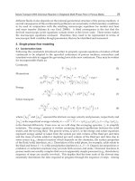
model and coordinate system is shown in Fig.4.
The x-axis is taken along the plate and the y-axis is normal to it. The wall is maintained at
constant temperature and concentration, T
w
and C
w
, respectively. The governing equations
for the steady state scenario [as given by (Mulolani & Rahman, 2000; El-Amin, 2004) may be
presented as:
Continuity:
∂u
∂x
+
∂v
∂y
= 0 (10)
30
Mass Transfer in Multiphase Systems and its Applications
Solute Transport With Chemical Reaction in Single- and Multi-Phase Flow in Porous Media 9
Fig. 4. Physical model and coordinate system.
Momentum:
u
c
√
K
ν

u
|
v
|
= −
K
μ

∂p
∂x
+ ρg

(11)
v
c
√
K
ν
v
|
v
|
= −
K
μ

∂p
∂y

(12)

Energy:
u
∂T
∂x
+ v
∂T
∂y
=
∂
∂x

α
x
∂T
∂x

+
∂
∂y

α
y
∂T
∂y

(13)
Solute transport:
u
∂C
∂x

+ v
∂C
∂y
=
∂
∂x

D
x
∂C
∂x

+
∂
∂y

D
y
∂C
∂y

−K
0
(
C −C
∞
)
n
(14)
Density

ρ
= ρ
∞
[
1 −β
∗
(T − T
∞
) − β
∗∗
(C − C
∞
)
]
(15)
Along with the boundary conditions:
y
= 0:v = 0, T
w
= const., C
w
= const.;
y
→ ∞ : u = 0, T → T
∞
,C → C
∞
(16)
where β
∗

is the thermal expansion coefficient β
∗∗
is the solutal expansion coefficient. It should
be noted that u and v refers to components of the volume averaged (superficial) velocity of the
fluid. The chemical reaction effect is acted by the last term in the right hand side of Eq. (14),
where, the power n is the order of reaction and K
0
is the chemical reaction constant. It is
assumed that the normal component of the velocity near the boundary is small compared
31
Solute Transport With Chemical Reaction in Singleand Multi-Phase Flow in Porous Media
10 Mass Transfer
with the other component of the velocity and the derivatives of any quantity in the normal
direction are large compared with derivatives of the quantity in direction of the wall. Under
these assumptions, Eq. (10) remains the same, while Eqs. (11)- (15) become:
u
+
c
√
K
ν
u
2
= −
K
μ

∂p
∂x
+ ρg


(17)
∂p
∂y
= 0 (18)
u
∂T
∂x
+ v
∂T
∂y
=
∂
∂y

α
y
∂T
∂y

(19)
u
∂C
∂x
+ v
∂C
∂y
=
∂
∂y


D
y
∂C
∂y

−K
0
(
C −C
∞
)
n
(20)
Following (Telles & V.Trevisan, 1993), the quantities of α
y
and D
y
are variables defined as
α
y
= α + γd
|
v
|
and D
y
= D + ζd
|
v

|
where, α and D are the molecular thermal and solutal
diffusivities, respectively, whereas γd
|
v
|
and ζd
|
v
|
represent dispersion thermal and solutal
diffusivities, respectively. This model for thermal dispersion has been used extensively (e.g.,
(Cheng, 1981; Plumb, 1983; Hong & Tien, 1987; Lai & Kulacki, 1989; Murthy & Singh, 1997)
in studies of non-Darcy convective heat transfer in porous media. Invoking the Boussinesq
approximations, and defining the velocity components u and v in terms of stream function ψ
as: u
= ∂ψ/∂y and v = −∂ψ/ ∂x, the pressure term may be eliminated between Eqs. (17) and
(18) and one obtains:
∂
2
ψ
∂y
2
+
c
√
K
ν
∂
∂y


∂ψ
∂y

2
=

Kgβ
∗
μ
∂T
∂y
+
Kgβ
∗∗
μ
∂C
∂y

ρ
∞
(21)
∂ψ
∂y
∂T
∂x
−
∂ψ
∂x
∂T

∂y
=
∂
∂y

α
+ γd
∂ψ
∂y

∂T
∂y

(22)
∂ψ
∂y
∂C
∂x
−
∂ψ
∂x
∂C
∂y
=
∂
∂y

D
+ ζd
∂ψ

∂y

∂C
∂y

−K
0
(
C −C
∞
)
n
(23)
Introducing the similarity variable and similarity profiles (El-Amin, 2004):
η
= Ra
1/2
x
y
x
, f
(η)=
ψ
αRa
1/2
x
,θ(η)=
T − T
∞
T

w
− T
∞
,φ(η)=
C −C
∞
C
w
−C
∞
(24)
The problem statement is reduced to:
f

+ 2F
0
Ra
d
f

f

= θ

+ Nφ

(25)
θ

+

1
2
f θ

+ γRa
d

f

θ

+ f

θ


= 0 (26)
φ

+
1
2
Le f φ

+ ζLe Ra
d

f

φ


+ f

φ


−Scλ
Gc
Re
2
x
φ
n=0
(27)
As mentioned in (El-Amin, 2004), the parameter F
0
= c
√
Kα/νd collects a set of parameters
that depend on the structure of the porous medium and the thermo physical properties of
the fluid saturating it, Ra
d
= Kgβ
∗
(T
w
− T
∞
)d/αν is the modified, pore-diameter-dependent
32

Mass Transfer in Multiphase Systems and its Applications
Solute Transport With Chemical Reaction in Single- and Multi-Phase Flow in Porous Media 11
Rayleigh number, and N = β
∗∗
(C
w
− C
∞
)/β
∗
ν is the buoyancy ratio parameter. With
analogy to (Mulolani & Rahman, 2000; Aissa & Mohammadein, 2006), we define Gc to be the
modified Grashof number, Re
x
is local Reynolds number, Sc and λ are Schmidt number and
non-dimensional chemical reaction parameter defined as Gc
= β
∗∗
g(C
w
− C
∞
)
2
x
3
/ν
2
, Re
x

=
u
r
x/ν, Sc = ν/D and λ = K
0
αd( C
w
− C
∞
)
n−3
/Kgβ
∗∗
, where the diffusivity ratio Le (Lewis
number) is the ratio of Schmidt number and Prandtl number, and u
r
=

gβ
∗
d(T
w
− T
∞
) is
the reference velocity as defined by (Elbashbeshy, 1997).
Eq. (27) can be rewritten in the following form:
φ

+

1
2
Le f φ

+ ζLe Ra
d

f

φ

+ f

φ


−χφ
n
= 0 (28)
With analogy to (Prasad et al., 2003; Aissa & Mohammadein, 2006), the non-dimensional
chemical reaction parameter χ is defined as χ
= ScλGc/Re
2
x
. The boundary conditions then
become:
f (0)=0,θ(0)=φ(0)=1, f

(∞)=θ(∞)=φ(∞)=0 (29)
It is noteworthy to state that F

0
= 0 corresponds to the Darcian free convection regime, γ = 0
represents the case where the thermal dispersion effect is neglected and ζ
= 0 represents
the case where the solutal dispersion effect is neglected. In Eq. (16), N
> 0 indicates the
aiding buoyancy and N
< 0 indicates the opposing buoyancy. On the other hand, from
the definition of the stream function, the velocity components become u
=(αRa
x
/x) f

and
v
= −(αRa
1/2
x
/2x)[ f − η f

]. The local heat transfer rate which is one of the primary interest
of the study is given by q
w
= −k
e
(∂T/∂y)|
y=0
, where, k
e
= k + k

d
is the effective thermal
conductivity of the porous medium which is the sum of the molecular thermal conductivity
k and the dispersion thermal conductivity k
d
. The local Nusselt number Nu
x
is defined as
Nu
x
= q
w
x/(T
w
− T
∞
)k
e
. Now the set of primary variables which describes the problem
may be replaced with another set of dimensionless variables. This include: a dimension
less variable that is related to the process of heat transfer in the given system which may
be expressed as Nu
x
/
√
Ra
x
= −[1 + γRa
d
F


(0)]θ

(0). Also, the local mass flux at the vertical
wall that is given by j
w
= −D
y
(∂C/∂y)|
y=0
defines another dimensionless variable that is the
local Sherwood number is given by, Sh
x
= j
w
x/(C
w
− C
∞
)D. This, analogously, may also
define another dimensionless variable as Sh
x
/
√
Ra
x
= −[1 + ζRa
d
F


(0)]φ

(0).
The details of the effects of all these parameters are presented in (El-Amin et al., 2008). We,
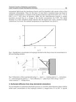
however, highlight the role of the chemical reaction on this system. The effect of chemical
reaction parameter χ on the concentration as a function of the boundary layer thickness η
and with respect to the following parameters: Le
= 0.5, F
0
= 0.3, Ra
d
= 0.7, γ = ζ = 0.0,
N
= −0.1 are plotted in Fig.5. This figure indicates that increasing the chemical reaction
parameter decreases the concentration distributions, for this particular system. That is,
chemical reaction in this system results in the consumption of the chemical of interest and
hence results in concentration profile to decrease. Moreover, this particular system also shows
the increase in chemical reaction parameter χ to enhance mass transfer rates (defined in
terms of Sherwood number) as shown in Fig.6. It is worth mentioning that the effects of
chemical reaction on velocity and temperature profiles as well as heat transfer rate may be
negligible. Figs. 7 and 8 illustrate, respectively, the effect of Lewis number Le on Nusselt
number and Sherwood number for various with the following parameters set as χ
= 0.02,
Ra
d
= 0.7, F
0
= 0.3, N = −0.1, γ = 0.0. The parameter ζ seems to reduce the heat transfer
rates especially with higher Le number as shown in Fig. 7. In the case of mass transfer rates
33

Solute Transport With Chemical Reaction in Singleand Multi-Phase Flow in Porous Media
12 Mass Transfer
0.0
0.2
0.4
0.6
0.8
1.0
0.0 0.5 1.0 1.5 2.0 2.5 3.0 3.5 4.0
K
I
F 
F 
F 
Fig. 5. Variation of dimensionless concentration with similarity space variable η for different
χ (Le
= 0.5, F
0
= 0.3, Ra
d
= 0.7, γ = ζ = 0.0, N = −0.1).
(defined in terms of Sherwood number), Fig. 8 illustrates that the parameter ζ enhances the
mass transfer rate with small values of Le

<1.55 and the opposite is true for high values of
Le

>1.55. This may be explained as follows: for small values of Le number, which indicates
0.2
0.4

0.6
0.8
1.0
0.00.51.01.52.02.53.03.54.0
Le
Sh
x
/(Ra
x
^0.5)
F 
F 
F 
F 
F 
Fig. 6. Effect of Lewis number on Sherwood number for various χ (F
0
= 0.3, Ra
d
= 0.7,
γ
= ζ = 0.0, N = −0.1).
34
Mass Transfer in Multiphase Systems and its Applications
Solute Transport With Chemical Reaction in Single- and Multi-Phase Flow in Porous Media 13
0.426
0.429
0.431
0.434
0.436

0.0 0.5 1.0 1.5 2.0 2.5 3.0 3.5 4.0
Le
Nu
x
/(Ra
x
^0.5)
] 
] 
] 
] 
Fig. 7. Variation of Nusselt number with Lewis number for various ζ (χ = 0.02, F
0
= 0.3,
Ra
d
= 0.7, γ = 0.0, N = −0.1).
that mass dispersion outweighs heat dispersion, the increase in the parameter ζ causes mass
dispersion mechanism to be higher and since the concentration at the wall is kept constant
this increases concentration gradient near the wall and hence increases Sherwood number. As
0.2
0.4
0.6
0.8
1.0
0.0 0.5 1.0 1.5 2.0 2.5 3.0 3.5 4.0
Le
Sh
x
/(Ra

x
^0.5)
] 
] 
] 
] 
Fig. 8. Effect of Lewis number on Sherwood number for various ζ (χ = 0.02, F
0
= 0.3,
Ra
d
= 0.7, γ = 0.0, N = −0.1).
35
Solute Transport With Chemical Reaction in Singleand Multi-Phase Flow in Porous Media
14 Mass Transfer
0.42
0.46
0.50
0.54
0.58
0.0 0.5 1.0 1.5 2.0 2.5 3.0 3.5 4.0
Le
Nu
x
/(Ra
x
^0.5)
J 
J 
J 

J 
Fig. 9. Variation of Nusselt number with Lewis number for various γ ( χ = 0.02, F
0
= 0.3,
Ra
d
= 0.7, ζ = 0.0, N = −0.1).
Le increases (Le
> 1), heat dispersion outweighs mass dispersion and with the increase in ζ
concentration gradient near the wall becomes smaller and this results in decreasing Sherwood
number. Fig. 9 indicates that the increase in thermal dispersion parameter enhances the heat
transfer rates.
6. Multi-phase flow modeling
Multi-phase systems in porous media are ubiquitous either naturally in connection with,
for example, vadose zone hydrology, which involves the complex interaction between three
phases (air, groundwater and soil) and also in many industrial applications such as enhanced
oil recovery (e.g., chemical flooding and CO
2
injection), Nuclear waste disposal, transport of
groundwater contaminated with hydrocarbon (NAPL, DNAPL), etc. Modeling of Multi-phase
flows in porous media is, obviously, more difficult than in single-phase systems. Here we
have to account for the complex interfacial interactions between phases as well as the time
dependent deformation they undergo. Modeling of compositional flows in porous media is,
therefore, necessary to understand a number of problems related to the environment (e.g.,
CO
2
sequestration) and industry (e.g., enhanced oil recovery). For example, CO
2
injection
in hydrocarbon reservoirs has a double benefit, on the one side it is a profitable method

due to issues related to global warming, and on the other hand it represents an effective
mechanism in hydrocarbon recovery. Modeling of these processes is difficult because the
several mechanisms involved. For example, this injection methodology associates, in addition
to species transfer between phases, some substantial changes in density and viscosity of the
phases. The number of phases and compositions of each phase depend on the thermodynamic
conditions and the concentration of each species. Also, multi-phase compositional flows
have varies applications in different areas such as nuclear reactor safety analysis (Dhir, 1994),
36
Mass Transfer in Multiphase Systems and its Applications
Solute Transport With Chemical Reaction in Single- and Multi-Phase Flow in Porous Media 15
high-level radioactive waste repositories (Doughty & Pruess, 1988), drying of porous solids
and soils (Whitaker, 1977), porous heat pipes (Udell, 1985), geothermal energy production
(Cheng, 1978), etc. The mathematical formulation of the transport phenomena are governed
by conservation principles for each phase separately and by appropriate interfacial conditions
between various phases. Firstly we give the general governing equations of multi-phase,
multicomponent transport in porous media. Then, we provide them in details with analysis
for two- and three-phase flows. The incompressible multi-phase compositional flow of
immiscible fluids are described by the mass conservation in a phase (continuity equation),
momentum conservation in a phase (generalized Darcy’s equation) and mass conservation
of component in phase (spices transport equation). The transport of N-components of
multi-phase flow in porous media are described by the molar balance equations. Mass
conservation in phase α :
∂
(φρ
α
S
α
)
∂t
= −∇·

(
ρ
α
u
α
)
+
q
α
(30)
Momentum conservation in phase α:
u
α
= −
Kk
rα
μ
α
(
∇
p
α
+ ρ
α
g∇z
)
(31)
Energy conservation in phase α:
∂
∂t

(
ρ
α
S
α
h
α
)
+ ∇·
(
ρ
α
u
α
h
α
)
= ∇·
(
S
α
k
α
∇T
)
+
¯
q
α
(32)

Mass conservation of component i in phase α:
∂
(φcz
i
)
∂t
+ ∇·
∑
α
c
α
x
αi
u
α
= ∇·

φD
i
α
∇(cz
i
)

+ F
i
, i = 1, ···, N (33)
where the index α denotes to the phase. S, p, q, u,k
r
,ρ and μ are the phase saturation, pressure,

mass flow rate, Darcy velocity, relative permeability, density and viscosity, respectively. c is
the overall molar density; z
i
is the total mole fraction of i
th
component; c
α
is the phase molar
densities; x
αi
is the phase molar fractions; and F
i
is the source/sink term of the i
th
component
which can be considered as the phase change at the interface between the phase α and other
phases; and/or the rate of interface transfer of the component i caused by chemical reaction
(chemical non-equilibrium). D
i
α
is a macroscopic second-order tensor incorporating diffusive
and dispersive effects. The local thermal equilibrium among phases has been assumed,
(T
α
= T,∀α), and k
α
and
¯
q
α

represent the effective thermal conductivity of the phase α and
the interphase heat transfer rate associated with phase α, respectively. Hence,
∑
α
¯
q
α
= q, q is
an external volumetric heat source/sink (Starikovicius, 2003). The phase enthalpy k
α
is related
to the temperature T by, h
α
=

T
0
c
pα
dT + h
0
α
. The saturation S
α
of the phases are constrained
by, c
pα
and h
0
α

are the specific heat and the reference enthalpy oh phase α, respectively.
∑
α
S
α
= 1 (34)
One may defined the phase saturation as the fraction of the void volume of a porous medium
filled by this fluid phase. The mass flow rate q
α
, describe sources or sinks and can be defined
by the following relation (Chen, 2007),
37
Solute Transport With Chemical Reaction in Singleand Multi-Phase Flow in Porous Media
16 Mass Transfer
q =
∑
j
ρ
j
q
j
δ(x − x
j
) (35)
q
= −
∑
j
ρ
j

q
j
δ(x − x
j
) (36)
The index j represents the points of sources or sinks. Eq. (35) represents sources and q
j
represents volume of the fluid (with density ρ
j
) injected per unit time at the points locations
x
j
, while, Eq. (36) represents sinks and q
j
represents volume of the fluid produced per unit
time at x
j
.
On the other hand, the molar density of wetting and nonwetting phases is given by,
c
α
=
N
∑
i=1
c
αi
(37)
where c
αi

is the molar densities of the component i in the phase α. Therefore, the mole fraction
of the component i in the respective phase is given as,
x
αi
=
c
αi
c
α
, i = 1, ···, N (38)
The mole fraction balance implies that,
N
∑
i=1
x
αi
= 1 (39)
Also, for the total mole fraction of i
th
component,
N
∑
i=1
z
i
= 1 (40)
Alternatively, Eq. (32) can be rewritten in the following form,
∂
∂t


φ
∑
α
c
α
x
αi
S
α

+ ∇·
∑
α
c
α
x
αi
u
α
= ∇·

φc
α
S
α
D
i
α
∇x
αi


+ F
i
, i = 1, ···, N (41)
F
i
may be written as,
F
i
=
∑
α
x
αi
q
α
, i = 1, ···, N (42)
where q
α
is the phase flow rate given by Eqs. (35), (36). From Eqs. (32) and (41), one may
deduce,
cz
i
=
∑
α
c
α
x
αi

S
α
=
∑
α
c
αi
S
α
, i = 1, ···, N (43)
If one uses the total mass variable X of the system (Nolen 1973; Young and Stephenson 1983),
X
=
∑
α
c
α
S
α
(44)
Therefore,
38
Mass Transfer in Multiphase Systems and its Applications
Solute Transport With Chemical Reaction in Single- and Multi-Phase Flow in Porous Media 17
1 =
∑
α
c
α
S

α
X
=
∑
α
C
α
(45)
where C
α
is the mass fraction phase α, respectively.
The quantity,
k
α
= Kk
rα
(46)
is known as effective permeability of the phase α. The relative permeability of a phase is a
dimensionless measure of the effective permeability of that phase. It is the ratio of the effective
permeability of that phase to the absolute permeability. Also, it is interesting to define the
quantities m
α
which is known as mobility ratios of phases α, respectively are given by,
m
α
=
k
α
μ
α

(47)
The capillary pressure is the the difference between the pressures for two adjacent phases α
1
and α
2
, given as,
p
cα
1
α
2
= p
α
1
− p
α
2
(48)
The capillary pressure function is dependent on the pore geometry, fluid physical properties
and phase saturations. The two phase capillary pressure can be expressed by Leverett
dimensionless function J
(S), which is a function of the normalized saturation S,
p
c
= γ

φ
K

1

2
J(S) (49)
The J
(S) function typically lies between two limiting (drainage and imbibition) curves which
can be obtained experimentally.
6.1 Two-phase compositional flow
The governing equations of two-phase compositional flow of immiscible fluids are given by,
Mass conservation in phase α:
∂
(φρ
α
S
α
)
∂t
= −∇·
(
ρ
α
u
α
)
+
q
α
α = w, n (50)
Momentum conservation in phase α:
u
α
= −

Kk
rα
μ
α
(
∇
p
α
+ ρ
α
g∇z
)
α = w, n (51)
Mass conservation of component i in phase α:
∂
(φcz
i
)
∂t
+ ∇·
(
c
w
x
wi
u
w
+ c
n
x

ni
u
n
)
=
F
i
, i = 1, ···, N (52)
where the index α denotes to the wetting (w) and non-wetting (n), respectively. S, p, q, u,k
r
,ρ
and μ are the phase saturation, pressure, mass flow rate, Darcy velocity, relative permeability,
density and viscosity, respectively. c is the overall molar density; z
i
is the total mole fraction
of i
th
component; c
w
, c
n
are the wetting- and nonwetting-phase molar densities; x
wi
, x
ni
are
the wetting- and nonwetting-phase molar fractions; and F
i
is the source/sink term of the i
th

component. The saturation S
α
of the phases are constrained by,
39
Solute Transport With Chemical Reaction in Singleand Multi-Phase Flow in Porous Media
18 Mass Transfer
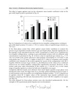
(a) Corey approximation (b) LET approximation
Fig. 10. Relative permeabilities.
S
w
+ S
n
= 1 (53)
The normalized wetting phase saturation S is given by,
S
=
S
w
−S
0w
1 −S
nr
−S
0w
0 ≤ S ≤ 1 (54)
where S
0w
is the irreducible (minimal) wetting phase saturation and S
nr
is the residual

(minimal) non-wetting phase saturation. The expression of relation between the relative
permeabilities and the normalized wetting phase saturation S, given as,
k
rw
= k
0
rw
S
a
(55)
k
rn
= k
0
rn
(1 −S)
b
(56)
The empirical parameters a and b can be obtained from measured data either by optimizing
to analytical interpretation of measured data, or by optimizing using a core flow numerical
simulator to match the experiment. k
0
rw
= k
rw
(S = 1) is the endpoint relative permeability to
water, and k
0
rn
= k

rn
(S = 0) is the endpoint relative permeability to the non-wetting phase.
For example, for the Corey power-law correlation, a
= b = 2, k
0
rn
= 1, k
0
rw
= 0.6, for water-oil
system see Fig.10a. Another example of relative permeabilities correlations is LET model
which is more accurate than Corey model. The LET-type approximation is described by three
empirical parameters L,E and T. The relative permeability correlation for water-oil system has
the form,
k
rw
=
k
0
rw
S
L
w
S
L
w
+ E
w
(1 −S)
T

w
(57)
and
k
rn
=
(
1 −S)
L
n
(1 −S)
L
n
+ E
n
S
T
n
(58)
The parameter E describes the position of the slope (or the elevation) of the curve. Fig. 10b
shows LET relative permeabilities with L
= E = T = 2 and k
0
rw
= 0.6 for water-oil system.
40
Mass Transfer in Multiphase Systems and its Applications
Solute Transport With Chemical Reaction in Single- and Multi-Phase Flow in Porous Media 19
Fig. 11. Capillary pressure as a function of normalized wetting phase saturation.
Also, there are Corey- and LET-correlations for gas-water and gas-oil systems similar to

the oil-water system. Correlation of the imbibition capillary pressure data depends on the
type of application. For example, for water-oil system, see for example, (Pooladi-Darvish &
Firoozabadi, 2000), the capillary pressure and the normalized wetting phase saturation are
correlated as,
p
c
= −B ln S (59)
where B is the capillary pressure parameter, which is equivalent to γ

φ
K

1
2
, in the general
form of the capillary pressure, Eq. (49), thus, B
≡−γ

φ
K

1
2
and J( S) ≡ lnS. Note that J(S) is
a scalar non-negative function. Capillary pressure as a function of normalized wetting phase
(e.g. water) saturation is shown in Fig. 11. Also, the well known (van Genuchten, 1980; Brooks
& Corey, 1964) capillary pressure formulae which can be written as,
p
c
= p

0
(S
−1/m
−1)
1−m
,0< m < 1 (60)
p
c
= p
d
S
−1/λ
, 0.2 < λ < 3 (61)
where p
0
is characteristic capillary pressure and p
d
is called entry pressure.
The capillary pressure p
c
is defined as a difference between the non-wetting and wetting phase
pressures,
p
c
= p
n
− p
w
(62)
the total velocity defined as,

41
Solute Transport With Chemical Reaction in Singleand Multi-Phase Flow in Porous Media
20 Mass Transfer
u = u
w
+ u
n
(63)
the total mobility is given by,
m
(S)=m
w
(S)+m
n
(S) (64)
the fractional flow functions are,
f
w
(S)=
m
w
(S)
m(S)
, f
n
(S)=
m
n
(S)
m(S)

(65)
and the density difference is,
Δρ
= ρ
n
−ρ
w
(66)
On the other hand, the molar density of wetting and nonwetting phases is given by,
c
w
=
N
∑
i=1
c
wi
, c
n
=
N
∑
i=1
c
ni
(67)
where c
wi
and c
ni

are the molar densities of component i in the wetting phase and nonwetting
phase phases, respectively. Therefore, the mole fraction of component i in the respective phase
is given as,
x
wi
=
c
wi
c
w
, x
ni
=
c
ni
c
n
, i = 1, ···, N (68)
The mole fraction balance implies that,
N
∑
i=1
x
wi
= 1,
N
∑
i=1
x
ni

= 1 (69)
Also, for the total mole fraction of i
th
component,
N
∑
i=1
z
i
= 1 (70)
Alternatively, Eq. (52) can be rewritten in the following form,
∂
∂t
[
φ
(
c
w
x
wi
S
w
+ c
n
x
ni
S
n
)]
+ ∇·

(
c
w
x
wi
u
w
+ c
n
x
ni
u
n
)
=
F
i
, i = 1, ···, N (71)
F
i
may be written as,
F
i
= x
wi
q
w
+ x
ni
q

n
, i = 1, ···, N (72)
where q
w
and q
n
are wetting phase and nonwetting phase phase flow rate, respectively. From
Eqs. (32) and (72), one may deduce,
cz
i
= c
w
x
wi
S
w
+ c
n
x
ni
S
n
= c
wi
S
w
+ c
ni
S
n

, i = 1, ···, N (73)
If one uses the total mass variable X of the system (Nolen, 1973; Young & Stephenson, 1983),
X
= c
w
S
w
+ c
n
S
n
(74)
42
Mass Transfer in Multiphase Systems and its Applications
Solute Transport With Chemical Reaction in Single- and Multi-Phase Flow in Porous Media 21
Therefore,
1
=
c
w
S
w
X
+
c
w
S
n
X
= C

w
+ C
n
(75)
where C
w
and C
n
are mass fractions of wetting- and nonwetting-phase of the system,
respectively. It is noted that,
C
w
= 1 −C
n
(76)
The total mole fraction of i
th
component, z
i
, in terms of one phase (wetting phase) mass
fraction and the wetting- and nonwetting-phase molar fractions, is given by,
z
i
= C
w
x
wi
+(1 −C
w
)x

ni
, i = 1, ···, N (77)
The pressure equation can be obtained, using the concept of volume-balance, as follows,
φC
f
∂p
∂t
+
N
∑
i=1
¯
V
i
∇·
(
c
w
x
wi
u
w
+ c
n
x
ni
u
n
)
=

N
∑
i=1
¯
V
i
F
i
, i = 1, ···, N (78)
where C
f
is the total fluid compressibility and V
i
is the total partial molar volume of the i
th
component. The distribution of the each component inside the two phases is restricted to
the stable thermodynamic equilibrium in terms of phases’ fugacities, f
wi
and f
ni
of the i
th
component. The stable thermodynamic equilibrium is given by minimizing the Gibbs free
energy of the system Bear (1972); Chen (2007),
f
wi
(p
w
, x
w1

, x
w2
,···, x
wN
)= f
ni
(p
n
, x
n1
, x
n2
,···, x
nN
), i = 1,···, N (79)
The fugacity of the i
th
component is defined by,
f
αi
= p
α
x
oi
φ
αi
, α = w,n, i = 1, ···, N (80)
φ
αi
,α = w, n is the fugacity coefficient of the i

th
component which will be defined below. The
phase and volumetric behaviors, including the calculations of the fugacities, are modeled
using the Peng-Robinson equation of state (Peng & Robinson, 1976). Introducing the pressure
of the phase, p
/
alpha, which is given by Peng-Robinson two-parameter equation of state as,
p
α
=
RT
V
α
−b
α
−
a
α
(T)
V
α
(V
α
+ b
α
)+b
α
(V
α
−b

α
)
, α = w,n (81)
a
α
=
N
∑
i=1
N
∑
j=1
x
iα
x
jα
(1 −κ
ij
)

a
i
a
j
, b
α
=
N
∑
j=1

x
iα
b
i
, α = w,n (82)
where R is the universal gas of constant, T is the temperature, V
α
is the molar volume of the
phase α, κ
ij
is a binary interaction parameter between the components i and j, a
i
and a
i
are
empirical factor for the pure component i given by,
a
i
= Π
ia
α
i
R
2
T
2
ic
p
ic
, b

i
= Π
ib
RT
ic
p
ic
, i = 1, ···, N (83)
T
ic
and p
ic
are the critical temperature and pressure,
43
Solute Transport With Chemical Reaction in Singleand Multi-Phase Flow in Porous Media
22 Mass Transfer
Π
ia
= 0.45724, Π
ib
= 0.077796, α
i
=

1
−λ
i

1
−


T
T
ic

2
,
λ
i
= 0.37464 + 1.5432ω
i
−0.26992ω
2
i
, i = 1, ···, N
(84)
Eq. (72) can be rewritten in the following cubic form,
Z
3
α
−(1 − B
α
)Z
2
α
+(A
α
−2B
α
−3B

2
α
)Z
α
−(A
α
B
α
− B
2
α
− B
2
α
)=0, α = w, n (85)
where Z
α
is the compressibility factor given by,
Z
α
=
b
α
V
α
RT
, α
= w, n (86)
(Chen, 2007) explained how to solve the cubic algebraic equation, Eq. (64). The fugacity
coefficient φ

αi
of the i
th
component is defined in terms of the compressibility factor Z
α
as,
lnφ
αi
=
b
i
b
α
(Z
α
−1) − ln(Z
α
− B
α
) −
A
α
2
√
2B
α

2
a
α

∑
N
j
=1
x
jα
(1 −κ
ij
)
√
a
i
a
j
−
b
i
b
α

·ln

Z
α
+(1+
√
2)B
α
Z
α

−(1−
√
2)B
α

(87)
Deriving of this equation can be found in details in (Chen, 2007).
Using Eqs. (51)- (53) and (62)- (65) with some mathematical manipulation one can find,
∂
(φρ
w
S
w
)
∂t
= −∇·ρ
w
f
w
(S)

Km
n
(S)

dp
c
dS
w
∇S

w
−Δρg∇z

+ u

+ q
w
(88)
Alternatively, in terms of pressure the flow equations may be rewritten in the form,
∂
(φρ
w
S
w
)
dp
c

∂p
n
∂t
−
∂p
w
∂t

= ∇·ρ
w

Kk

rw
μ
w
(
∇
p
w
−ρ
w
g∇z
)

+ q
w
(89)
∂
(φρ
n
(1 −S
w
))
dp
c

∂p
n
∂t
−
∂p
w

∂t

= ∇·ρ
n

Kk
rn
μ
n
(
∇
p
n
−ρ
n
g∇z
)

+ q
n
(90)
Both models, Eq. (88) and Eqs. (89)- (90) are used intensively especially in the field of oil
reservoir simulations.
6.2 Three-phase compositional flow
In three-phase compositional flow the governing equations will not has a big difference from
the two-phase case. In this section we introduce the main points which distinguish the
three-phase flow. On the other hand, we consider the black oil model as an example of the
three-phase compositional flow instead of considering the general case to investigate such
kind of complex flow. The black oil model is water-oil-gas system such that water represents
the aqueous phase and oil represents oleic phase. The hydrocarbon in a reservoir is almost

consists of oil and gas. Water is being naturally in the reservoir or injected in the secondary
stage of oil recovery. Also, gas may be found naturally or/and injected as CO
2
injection for
the enhanced oil recovery stage. The governing equations may be extended to the three-phase
flow. The generalized Darcy’s law with mass transfer equations will remain the same as
in Eqs. (30) and (31) with considering α
= w,o, g, thus each phase is represented by two
equations, continuity and momentum. The index α denotes to the water (w), oil (o) and gas (g),
respectively. The solute transport equations is modified to suite the three-phase compositional
flow as follow,
44
Mass Transfer in Multiphase Systems and its Applications
Solute Transport With Chemical Reaction in Single- and Multi-Phase Flow in Porous Media 23
∂(φcz
i
)
∂t
+ ∇·

c
w
x
wi
u
w
+ c
o
x
oi

u
o
+ c
g
x
gi
u
g

= F
i
, i = 1, ···, N (91)
or
∂
∂t

φ

c
w
x
wi
S
w
+ c
o
x
oi
S
o

+ c
g
x
gi
S
g

+ ∇·

c
w
x
wi
u
w
+ c
o
x
oi
u
o
+ c
g
x
gi
u
g

=
x

wi
q
w
+ x
oi
q
o
+ x
gi
q
g
, i = 1, ···, N
(92)
Following (Stone, 1970; 1973) we assume that the water-oil and oil-gas relative permeabilities
are given as the two-phase case,
k
rw
(S
w
)=k
0
rw

S
w
−S
wc
1 −S
wc
−S

orw

n
w
(93)
k
rg
(S
g
)=k
0
rg

S
g
−S
gr
1 −S
wc
−S
org
−S
gr

n
g
(94)
where S
wc
is the connate water saturation, S

org
is the residual oil saturation to gas, S
orw
is the
residual oil saturation to water, S
gr
is the residual gas saturation to water. S
w
= 1 −S
orw
. The
intermediate-wetting phase (oil phase) relative permeabilities are given by,
k
row
(S
w
)=k
0
row

1
−S
w
−S
orw
1 −S
wc
−S
orw


n
ow
(95)
k
ro g
(S
g
)=k
0
ro g

1
−S
wc
−S
org
−S
g
1 −S
wc
−S
org
−S
gr

n
og
(96)
The intermediate-wetting phase relative permeability is given by,
k

ro
(S
w
,S
g
)=
k
row
k
ro g
k
norm
(97)
k
norm
may be setting as one or given by another formula as in the literature which will not
mention here for breif.
6.3 Numerical methods for multi-phase flow
Much progress in the last three decades in numerical simulation of multi-phase flow with
compositional and chemical effect. Both first-order finite difference and finite volume
methods are used. First-order finite difference schemes has numerical dispersion issue, while
the first-order finite volume has powerful features when used for two-phase flow simulation
(Leveque, 2002). However, the later one has some limitations when applied to fractured
media (Monteagudo & Firoozabadi, 2007). Also, higher-order methods have less numerical
dispersion and more accurate flow field calculations than the first-order methods. The
combined mixed-hybrid finite element (MHFE) and discontinuous Galerkin (DG) methods
have been used to simulate two-phase flow by (Hoteit & Firoozabadi, 2005; 2006; Mikyska
& Firoozabadi, 2010). In the combined MHFE-DG methods, MHFE is used to solve the
pressure equation with total velocity, and DG method is used to solve explicitly the species
transport equations. Therefore, the parts are coupled using scheme such as the iterative

IMplicit Pressure and Explicit Concentration (IMPEC) scheme. Also, (Sun et al., 2002) have
used combined MHFE-DG methods to miscible displacement problems in porous media.
45
Solute Transport With Chemical Reaction in Singleand Multi-Phase Flow in Porous Media
24 Mass Transfer
The DG method (Wheeler, 1987; Sun & Wheeler, 2005a;b; 2006) is derived from variational
principles by integration over local cells, thus it is locally mass conservative by construction.
In addition, the DG method has low numerical diffusion because higher-order approximations
are used within cells and the cells interfaces are weakly enforced through the bilinear form.
DG method is efficiently implementable on unstructured and nonconforming meshes.
The MHFE methods are based on a variational principle expressing an equilibrium or saddle
point condition that can be satisfied locally on each element (Brezzi & Fortin, 1991). It has
an indefinite linear system of equations for pressure (scalar) and the total velocity (vector)
but they definitized by appending as extra degrees of freedom the average pressures at the
element edges.
7. References
Aissa, W. A. & Mohammadein, A. A. (2006). Chemical reaction effects on combined forced
and free convection flow of water at 4 c past a semi-infinite vertical plate, J. Eng. Sci.
Assiut Univ. 34: 1225–1237.
Bear, J. (1972). Dynamics of Fluids in Porous Media, Elsevier, New York.
Brezzi, F. & Fortin, M. (1991). Mixed and hybrid finite element methods, Springer–Verlag, New
York.
Brooks, R. H. & Corey, A. T. (1964). Hydraulic properties of porous media, Hydrology Papers 3.
Chen, Z. (2007). Reservoir simulation: mathematical techniques in oil recovery, SIAM, USA.
Cheng, P. (1978). Heat transfer in geothermal systems, Advances in Heat Transfer 14: 1–105.
Cheng, P. (1981). Thermal dispersion effects on non-darcy convection flows in a saturated
porous medium, Lett. Heat Mass Transfer 8: 267–270.
Dhir, V. K. (1994). Boiling and two-phase flow in porous media, Annu. Rev. Heat Transfer
5: 303–350.
Doughty, C. & Pruess, K. (1988). A semianalytical solution for heat-pipe effects near high-level

nuclear waste packages buried in partially saturated geological media, Int. J. Heat
Mass Transfer 31: 79–90.
El-Amin, M. F. (2004). Double dispersion effects on natural convection heat and mass transfer
in non-darcy porous medium, Appl. Math. Comp. 156: 1–17.
El-Amin, M. F., Aissa, W. A. & Salama, A. (2008). Effects of chemical reaction and double
dispersion on non-darcy free convection heat and mass transfer, Transport in Porous
Media 75: 93–109.
Elbashbeshy, E. M. A. (1997). Heat and mass transfer along a vertical plate with variable
surface tension and concentration in the presence of magnetic field, Int. J. Eng. Sci.
Math. Sci. 4: 515–522.
Hassanizadeh, S. M. & Gray, W. (1979a). General conservation equations for multi-phase
systems 2. mass, momenta, energy and entropy equations, Advances in Water
Resources 2: 191–208.
Hassanizadeh, S. M. & Gray, W. (1980). General conservation equations for multi-phase
systems 3. constitutive theory for porous media, Advances in Water Resources 3: 25–40.
Hassanizadeh, S. M. & Gray, W. G. (1979b). General conservation equations for multi-phase
systems 1. averaging procedure, Advances in Water Resources 2: 131–144.
Herwig, H. & Koch, M. (1991). Natural convection momentum and heat transfer in saturated
highly porous mediaan asymptotic approach, Heat Mass Transfer 26: 169–174.
Hong, J. T. & Tien, C. L. (1987). Analysis of thermal dispersion effect on vertical plate natural
convection in porous media, Int. J. Heat Mass Transfer 30: 143–150.
46
Mass Transfer in Multiphase Systems and its Applications
Solute Transport With Chemical Reaction in Single- and Multi-Phase Flow in Porous Media 25
Hoteit, H. & Firoozabadi, A. (2005). Multicomponent fluid flow by discontinuous galerkin
mand mixed methods in unfractured and fractured media, Water Resour. Res.
41: W11412.
Hoteit, H. & Firoozabadi, A. (2006). Compositional modeling by the combined discontinuous
galerkin mand mixed methods, SPE Journal .
Lai, F. C. & Kulacki, F. A. (1989). Thermal dispersion effect on non-darcy convection from

horizontal surface in saturated porous media, Int. J. Heat Mass Transfer 32: 971–976.
Leal, L. G. (2007). Advanced transport phenomena, Cambridge University Press.
Leveque, R. J. (2002). Finite volume methods for hyperbolic problems, Cambridge Texts in Applied
Mathematics, Cambridge University Press.
Mikyska, J. & Firoozabadi, A. (2010). Implementation of higher-order methods for robust and
efficient compositional simulation, J. Comput. Physics 229: 2898–2913.
Monteagudo, J. E. P. & Firoozabadi, A. (2007). Control-volume model for simulation of
water injection in fractured media: incorporating matrix heterogeneity and reservoir
wettability effects, SPE Journal .
Mulolani, I. & Rahman, M. (2000). Similarity analysis for natural convection from a vertical
plate with distributed wall concentration, Int. J. Math. Math. Sci. 23: 319–334.
Murthy, P. V. S. N. & Singh, P. (1997). Thermal dispersion effects on non-darcy natural
convection with lateral mass flux, Heat Mass Transfer 33: 1–5.
Nolen, J. S. (1973). Numerical simulation of compositional phenomena in petroleum
reservoirs, Reprint Series, SPE, Dallas, 11, 268284.
Peng, D Y. & Robinson, D. B. (1976). A new two-constant equation of state, Industrial and
Engineering Chemistry Fundamentals 15: 59–64.
Plumb, O. A. (1983). The effect of thermal dispersion on heat transfer in packed bed boundary
layers, In: Proc. 1st ASME/JSME Thermal Engng. Joint Conf., Vol. 2, pp. 17–21.
Pooladi-Darvish, M. & Firoozabadi, A. (2000). Co-current and counter-current imbibition in a
water-wet matrix block, SPE Journal 5: 3–11.
Prasad, K. V., Abel, S. & Datti, P. S. (2003). Diffusion of chemically reactive species of a
non-newtonian fluid immersed in a porous medium over a stretching sheet, Int. J.
Non-Linear Mech. 38: 651–657.
Salama, A. & van Geel, P. J. (2008a). Flow and solute transport in saturated porous media: 1
the continuum hypothesis, J Porous Media 11: 403–413.
Salama, A. & van Geel, P. J. (2008b). Flow and solute transport in saturated porous media: 2
violating the continuum hypothesis, J Porous Media 11: 421–441.
Starikovicius, V. (2003). The multiphase fl ow and heat transfer in porous media, Berichte des
Fraunhofer ITWM 55: 1–30.

Stone, H. (1970). Probability model for estimating three-phase relative permeability, JPT 214.
Stone, H. (1973). Estimation of three-phase relative permeability and residual oil data, J. Cdn.
Pet. Tech. 13: 53.
Sun, S., Riviere, B. & Wheeler, M. F. (2002). A combined mixed finite element and
discontinuous galerkin method for miscible displacement problems in porous media,
Proceedings of International Symposium on Computational and Applied PDEs, Zhangjiajie
National Park of China, 321-341.
Sun, S. & Wheeler, M. F. (2005a). Discontinuous galerkin methods for coupled flow and
reactive transport problems, Appl. Num. Math. 52: 273–298.
Sun, S. & Wheeler, M. F. (2005b). Symmetric and nonsymetric discontinuous galerkin methods
for reactive transport in porous media, SIAM J. Numer. Anal. 43: 195–219.
47
Solute Transport With Chemical Reaction in Singleand Multi-Phase Flow in Porous Media
26 Mass Transfer
Sun, S. & Wheeler, M. F. (2006). Analysis of discontinuous galerkin methods for
multi-components reactive transport problem, Comput. Math. Appl. 52: 637–650.
Telles, R. S. & V.Trevisan, O. (1993). Dispersion in heat and mass transfer natural convection
along vertical boundaries in porous media, Int. J. Heat Mass Transfer 36: 1357–1365.
Udell, K. S. (1985). Heat transfer in porous media considering phase change and capillarity –
the heat pipe effect, Int. J. Heat Mass Transfer 28: 485–495.
van Genuchten, M. (1980). A closed-form equation for predicting the hydraulic conductivity
of unsaturated soils, Soil Sci. Soc. Am. J. 44: 892–898.
Wheeler, M. F. (1987). An elliptic collocation finite element method with interior penalties,
SIAM J. Numer. Anal. 15: 152–161.
Whitaker, S. (1967). Diffusion and dispersion in porous media, AIChE 13: 420–427.
Whitaker, S. (1977). Simultaneous heta, mass, and momentum transfer in porous media: A
theory of drying, Advances in Heat Transfer 13: 119–203.
Young, L. C. & Stephenson, R. E. (1983). A generalized compositional approach for reservoir
simulation, SPE Journal 23: 727–742.
48

Mass Transfer in Multiphase Systems and its Applications
0
Multiphase Modelling of Thermomechanical
Behaviour of Early-Age Silicate Composites
Ji
ˇ
r
´
ı Vala
Brno University of Technology, Faculty of Civil Engineering
Czech Republic
1. Introduction
The reliable prediction of thermomechanical behaviour of early-age silicate composites is
a complicated multiphysical and multiscale problem, containing a lot of open questions.
However, silicate mixtures, namely fresh concrete, are the most commonly used materials
in building constructions throughout the world, thus such prediction is of great practical
significance. The most important modelling outputs are the macroscopic effective strain,
stress, temperature, moisture etc. time evolutions, driven by chemical reactions of particular
clinker minerals with water. Every realistic model is then expected to include thermo-, chemo-
and hygromechanical processes and phase changes, involving all available microstructural
information related to the real porous medium.
The deformation of a material sample or a building construction made from silicate
composites has to be analyzed at least as the superposition of
– reversible elastic deformation,
– viscous material flow,
– volume changes, unlike remaing contributions independent of external loads.
The crucial external and internal influences are:
– internal hydration heat, generated by the hydration hydraulic processes,
– ambient temperature variation, connected with ambient humidity variation (natural or
artificial ones),

– external mechanical loads.
The significant physical (and chemical) processes are:
a) thermal deformation,
b) autogenous shrinkage,
c) carbonation,
d) elastic and creep deformation,
e) additional thermal deformation,
f) drying shrinkage and swelling.
3
2 Mass Transfer
In the first period of intense hydration a), accompanied by b), is dominant. In the later
period the role of a) decreases, but the effect of c) has to be taken into account. The external
mechanical loads cause d) (creep especially in the earliest age), the external temperature
changes simultaneously force e), modified by f).
The traditional approach to the modelling of such complex physical and technical problems
is the phenomenological one, as discussed in (Ba
ˇ
zant, 2001): the effect of changes of density,
porosity, permeability, compressive strength, etc. on material behaviour is lumped together to
some model parameters, which must be identified by long-lasting tests in the whole range of
model applicability. On the contrary, the so-called CCBM (“Computational Cement-Based
Material”) approach, suggested in (Maruyama et al., 2001), develops the original idea of
(Tomosawa, 1997): the slight generalization of its (seemingly simple) form
˙

= Φ(,
∗
),
˙


∗
= Ψ(,
∗
)
where  is the radius of an unhydrated cement particle, 
∗
its total radius including hydrate,
dot symbols refer (everywhere in this chapter) to derivatives with respect to the time t
≥ 0
and Φ, Ψ are (in general rather complicated) material characteristics with hidden , 
∗
(but
not with their time derivatives) again. The analysis of (Maruyama et al., 2001) assumes ideal
spherical particles, hydration products adherent to such particles (whose size distribution is
approximated by a special Rosin-Ramler function), water diffusing through the hydrate layer
and chemically reacting with cement, up to interparticle contact effects; the amount of water is
controlled by the pore structure, modified by hydration reactions of cement constituents and
corresponding heat generation. Particular cement constituents, namely alite (C
3
S, typically 65
% of the total mass in the Portland cement), belite (C
2
S, 15 %), aluminate phase (C
3
A, 7 %),
ferrite phase (C
4
AF, 8 %), etc., have their own densities and hydration reactions, generating
hydration heat.
For various types of cement we have different hydration degree Γ, introduced as

Γ :
=
μ
h
μ
h
∞
where μ
h
denotes the (usually increasing) mass of skeleton (and corresponding sink of liquid
water mass) ans μ
h
∞
the final mass of hydrated (chemically combined) water in a volume unit;
alternatively (cf. (Gawin et al., 2006a), p. 309)
Γ :
=
Q
h
Q
h
∞
in terms of the heat Q
h
released during hydration and of its final value Q
h
∞
. However, it
is difficult to guarantee above sketched model assumption in building practice, applying
also (not single-sized) additional aggregate; thus Γ is usually quantified from macroscopic

experiments (as adiabatic calorimetric or isothermal strength evolution tests) not from such
microstructural considerations. Consequently Γ can be evaluated by (Gawin et al., 2006a),
p. 309, from an auxiliary evolution problem of type
˙
Γ
= A( Γ,φ, T)
with an a priori known real function A.
50
Mass Transfer in Multiphase Systems and its Applications
Multiphase Modelling of Thermomechanical Behaviour of Early-Age Silicate Composites 3
During the same hydration process the non-negligible vapour mass source μ
e
, caused by the
liquid water evaporation or desorption, occurs, too. Unfortunately, unlike μ
h
, no reasonable
constitutive relation is available for the direct evaluation of μ
e
.
Clearly, the reliable prediction of material behaviour applicable to real building objects during
hydration needs some multiscale analysis. The mechanistic approach (Pichler et al., 2007)
makes it possible to consider above sketched effects explicitly because they appear directly in
the model equations, distinguishing between 4 length scales, characterized as
I) anhydrous-cement scale (typical length of a representative volume element from 10-8 to
10-6 m), in more details decomposed into 3 subscales, where the qualitative estimate of
activity of four main clinker phases, water and air requires the detailed micromechanical
evaluation of corresponding chemical reactions,
II) cement-paste scale (from 10
−6
to 10

−4
m),
III) mortar scale (about 10
−2
m),
IV) macroscale (about 10
−1
m).
The analysis of capillary depression at scale I) (considering membrane forces on solid/liquid,
solid/gas and liquid/gas interfaces), of ettringite formation at scale II), of autogenous
deformation at scales II) and III), referring to the Hill homogenization lemma (see (Dormieux
et al., 2006), p. 105), must be completed by the interpretation of such multiscale results at
scale IV). However, different physical and chemical processes studied at particular scales do
not admit proper and physically transparent mathematical analysis of two- and more-scale
convergence, as discussed in (Cioranescu & Donato, 1999), (Vala, 2006) or (Efendiev et
al., 2009), including its non-periodic (formally complicated) generalization, introduced in
(Nguentseng, 2003-4).
The approach (Gawin et al., 2006a) applies certain mechanistic-type method to obtain the
governing equations only, using the averaging hybrid mixture theory: the developments starts
at the micro-scale and balance equations for particular phases and interfaces are introduced
at this level and then averaged for obtaining macroscopic balance equations. Four phases are
distinguished: solid skeleton, liquid water, vapour and dry air, whose densities are considered
(under the passive air assumption) as constants; the whole hygro-thermo-chemo-mechanical
process is then studied as the time evolution of capillary pressure, gas pressure, temperature
and displacement of points related to the reference (initial) configuration, driven by balance
equations of classical thermodynamics and conditioned by corresponding constitutive laws.
The detailed geometrical analysis (Sanavia et al., 2002) (without phase changes) offers the
possibility to extend such considerations beyond the assumption of small deformations and
involve some elements of fracture mechanics.
The development, laboratory testing and computational simulations of new materials, namely

those for the application of advanced engineering structures, belong to the research priorities
of the Faculty of Civil Engineering of Brno University of Technology. Moreover, these
activities should be intensified thanks to the proposed complex research institution AdMaS
(“Advanced Materials and Structures”) in the near future. The long-time behaviour of
massive structures, especially its bearing value, durability and user properties, is typically
conditioned by the early-age heat, moisture, etc. treatment, modified by foundations,
subgrades, reinforcement and connecting members; thus the aim is to design the whole
building process to minimize the development of significant tensile stresses to avoid the
the danger of cracking, or even to force volume changes and corresponding final stresses
appropriate for the future use of a structure. The deeper understanding of decissive
51
Multiphase Modelling of Thermomechanical Behaviour of Early-Age Silicate Composites
4 Mass Transfer
processes in early-age materials that effects volume changes is therefore needed, although
no closed physical and mathematical models are available and all simplified calculations
contain empirical parameters and functions, whose identification, supported by laboratory
measurements or in situ observations, generates separate non-trivial problems, not discussed
in details here. However, we shall demonstrate how the thermomechanical analysis of balance
of mass, (linear and angular) momentum and energy for computational HAM (“heat, air and
moisture”) models in civil engineering is able to be extended to a complex computational
model, including the mass source or solid skeleton related to the hydration process (and
corresponding sink of liquid water mass), as well as the vapour mass source caused by the
liquid water evaporation or desorption, using some micromechanical arguments from the
theory of porous media.
2. Mixture components
To analyze the phase changes in an early-age silicate composite, we shall consider four
material phases:
– solid material, identified by an index s ,
– liquid water, identified by an index w,
– water vapour, identified by an index v,

– dry air, identified by an index a.
In addition to partial derivatives of scalar quantities ψ with respect to time, i. e.
˙
ψ :
= ∂ψ/∂t ,
we shall introduce also the partial derivatives of such quantities with respect to x
i
, i ∈{1,2,3},
x
=(x
1
, x
2
, x
3
) being a Cartesian coordinate system in the three-dimensional Euclidean space
R
3
,
ψ
,i
:= ∂ψ/∂x
j
.
In the case of real vector variables with values in
R
3
we shall write ψ briefly instead of
(ψ
1

,ψ
2
,ψ
3
). Even in the case of matrix variables in the with values in R
3×3
, the space of real
matrices of the third order, we shall write ψ only instead of ψ
ij
, i, j ∈{1,2,3}. Consequently,
due to the preceding notation, unlike the matrix elements ψ
ij
from ψ ∈R
3×3
with i, j ∈{1,2,3},
we have e. g. for ψ
∈R
3
ψ
i,j
:= ∂ψ
i
/∂x
j
.
We shall assume that the scale bridging between particular scales (if relevant scale material
data are available) can be done by means of the averaging of model variables. The basic
(averaged) variables in our model, related to a representative volume element, are:
– 4 intrinsic phase densities R
=(ρ

s
,ρ
w
,ρ
v
,ρ
a
),
– 12 components of phase velocities V
=(v
s
i
,v
w
i
,v
v
i
,v
a
i
) with i ∈{1, 2,3},
– 3 fluid pressures P
=(p
w
, p
v
, p
a
),

– 1 (absolute) temperature ϑ.
52
Mass Transfer in Multiphase Systems and its Applications
Multiphase Modelling of Thermomechanical Behaviour of Early-Age Silicate Composites 5
Intrinsic phase densities evidently do not reflect the amount of particular phases in a volume
unit; thus it is useful to define (real) phase densities
ρ
ε
:= η
ε
ρ
ε
formally for any phase index ε ∈{s, w,v, a} where
η
s
=(1 −n),
η
w
= ns,
η
v
= n(1 − s),
η
a
= n(1 − s)(1 − φ) .
Unfortunately it is not easy to evaluate the porosity n, the saturation degree s and the relative
humidity (the volume fraction occupied by water vapour in the total gaseous phase) φ.
Nevertheless, similarly to ρ
ε
, ε ∈{s, v,w, a}, being motivated by the Dalton law by (Berm

´
udez
de Castro, 2005), p. 111, we can also introduce pressures
p
ε
:= η
ε
p
ε
.
We can evaluate also the “macroscopic” mixture density
ρ :
= ρ
s
+ ρ
w
+ ρ
v
+ ρ
a
.
Let us also remark that, from he point of view of solid phase, fluid pressures P are
accompanied by a (partial) Cauchy stress tensor compound from components τ
ij
with i, j ∈
{
1,2,3}, whose (indirect) relation to V will be discussed later.
The porosity can be evaluated from the finite strain analysis by (Sanavia et al., 2002), p. 139.
The multiphase medium at the macroscopic level can be described as the superposition of all
phases ε, whose material point with coordinates x

ε0
i
in the reference configuration Ω in R
3
occupies a point with coordinates x
ε
i
(t); zero indices are related to the reference configuration,
here in the initial time t
= 0. In the Lagrangian description of the motion the position of each
material point can be expressed as
x
ε
i
(t)=x
ε0
i
+ u
ε
i
(x
ε0
i
,t)
where u
ε
i
(x
ε0
i

,t) denotes the displacement at chosen time and zero indices are related to a
reference configuration, here in time t
= 0. Thus
F
ε
ij
(x
ε0
,t) :=
∂x
ε
i
(x
ε0
)
∂x
ε0
j
= δ
ij
+
∂u
ε
i
(x
ε0
,t)
∂x
ε0
j

can be taken as a deformation characteristic, δ being a Kronecker symbol, consequently
n
= 1 −(1 −n
0
)
(
det F
s
)
−1
where n
0
(x
s0
) denotes the porosity in the reference configuration. In the linearized geometry
this access in not available: e. g. (Gawin et al., 2006a), p. 310 presents an empirical
(nearly linear) function n
(Γ), justified by the correlation analysis, exploiting the experimental
database of (De Schutter, 2002) where hardening cement pastes with 5 different values of
water/cement ratio are studied.
53
Multiphase Modelling of Thermomechanical Behaviour of Early-Age Silicate Composites