Self Organizing Maps Applications and Novel Algorithm Design Part 5 docx
Bạn đang xem bản rút gọn của tài liệu. Xem và tải ngay bản đầy đủ của tài liệu tại đây (2.34 MB, 40 trang )
is, pairs of staring and ending of viewing, SOM must accepts range data as inputs. The other
is that the starting and ending points of viewing do not necessarily come in a pair to a server
computer as pointed out in Ishikawa et al. (2007).
To make matters worse, starting data and ending data from the same client computer do not
necessarily have the same identification code, so that it is difficult to match the starting data
and ending data from the same client computer. If we could assign identification code to the
client computer, we could solve the problem. One possible ID is the IP address of the client
computer, but IP addresses of many computers are assigned dynamically so that they may
change between the starting of viewing and the end of viewing. The other possible ID is a
cookie that would be set in a multimedia player and referred to by a server computer, but
cookies by multimedia players are not popular and not standardized yet.
Since the advantages of SOM are indispensable, we devised two new methods, both of
them consist of networks and their learning algorithm based on the conventional SOM.
The proposed method described in section 3.2 has an SOM-like network that accepts
starting points and ending points independently, that is, in any order without identifying
its counterpart and learns viewing frequency distribution. The one in section 3.3 has two
SOM-like networks, each of which accept one of starting and ending points and learn
independently and one more SOM-like network that learns viewing frequency distribution
from the former networks.
Our purpose is to recover frequency distribution of viewing events from their start and end
events. In this section, we focus on equal density partition x
0
< x
1
< ··· < x
n
of frequency
distribution p
(x) such that
x
i+1
x
i
p(x) dx is a constant independent of i.
The proposed algorithm is shown in Fig. 4. Corresponding to the type of posi ti on
(t) and
operation
(t) of network input (see Equation 2), the values of neurons, i.e., positions are
updated (lines 10–31, 40). Since an update step α is a constant, a neuron might move past
a neuron next to it. To prevent this, a neuron should maintain a certain distance (ε)from
the neuron next to it (lines 32–39). Derivation of update formulae is as follows: Consider
one-dimensional SOM-like network
X
X =
x
1
, ,x
n
, x
1
< x
2
< ··· < x
n
∈
1
.
If
X is arranged such that for some c
x
i+1
x
i
p(x) dx = c,
then clearly
X reflects the density function p(x) in such a way that
c
x
i+1
− x
i
≈ p(x),forx ∈ [x
i
, x
i+1
].
Suppose that p
(x) is sufficiently smooth and for simplicity the sign of ∂p /∂x does not change
in
(x
i
, x
i+1
). Then, by putting y = p(x),
150
Self Organizing Maps - Applications and Novel Algorithm Design
1: initialize network Y←Y
0
= y
0
1
, ,y
0
|Y|
, y
0
1
< y
0
2
< ···< y
0
|Y|
2: t ← 0
3: repeat forever
4: t
← t + 1
5: receive operation information R
(t)=x(t), op(t)
6: B = b
0
← 0, b
1
← y
1
, ,b
|Y|
← y
|Y|
,b
|Y|+1
← sup(Y)
7: for i ∈{1,2,. . . ,|Y|}
8: Δ
i
← 0
9: end for
10: if op
(t)=1 then
11: for i
∈{2,3, . ,|Y| − 1}
12: if x(t) < b
i
then
13: Δ
i
← 2y
i
− b
i+2
− b
i
14: elseif x(t) < y
i
then
15: Δ
i
← 2y
i
− b
i+2
− x(t)
16: elseif x(t) < y
i
then
17: Δ
i
← b
i+2
− x(t)
18: end if
19: end for
20: else
21: for i
∈{2,3, . ,|Y| − 1}
22: if x(t) < b
i
then
23: Δ
i
←−(2y
i
− b
i+2
− b
i
)
24: elseif x(t) < y
i
then
25: Δ
i
←−
2y
i
− b
i+2
− x(t)
26: elseif x
(t) < y
i
then
27: Δ
i
←−
b
i+2
− x(t)
28: end if
29: end for
30: end if
31:
Z = z
1
, ,z
|Y|
←Y+ αΔ
32: for i
∈{2, 3, , |Y| − 1}
33: if z
i
≤ y
i−1
then
34: z
i
← y
i−1
+ ε
35: end if
36: if z
i
≥ y
i+1
then
37: z
i
← y
i+1
− ε
38: end if
39: end for
40:
Y←Z
41: end repeat
Fig. 4. Procedures of the proposed in section 3.2
151
Self-Organization and Aggregation of Knowledge
x
n
x
0
p(x) dx
=
p(x
n
)
p(x
0
)
y
∂p
−1
∂y
dy
= p
−1
(y) y
p(x
n
)
p(x
0
)
−
p(x
n
)
p(x
0
)
p
−1
(y) dy
=
x
n
p(x
n
) − x
0
p(x
0
)
−
n−1
∑
i=0
p(x
i+1
)
p(x
i
)
p
−1
(y) dy
=
x
n
p(x
n
) − x
0
p(x
0
)
−
n−1
∑
i=0, x
i
≤∃x≤x
i+1
p
(x
i+1
) − p(x
i
)
x
=(x
n
− x
0
) p(x
0
)+
n−1
∑
i=0, x
i
≤∃x≤x
i+1
p
(x
i+1
) − p(x
i
)
(x
n
− x).
Hereafter p
(x
0
)=0 is assumed. If increment or decrement events, as Equation 3 or 4, Δp(x)
occur such that
∂p
∂x
Δx
≈ E[Δp(x)],forx ∈ [x
0
, x
n
],
then
x
n
x
0
p(x) dx ≈ E[Δp(x)(x
n
− x)].
Therefore if we could arrange
X such that for x ∈ [x
i
, x
i+1
)
E[Δp(x)(x
n
− x)]
isaconstantindependentofi, X is the one we want. From this we get the following update
formulae for x
i
x
i
← x
i
+ αΔx
i
,
where
Δx
i
=
⎧
⎪
⎪
⎪
⎪
⎪
⎨
⎪
⎪
⎪
⎪
⎪
⎩
Δp
(x
i+1
− x
i
) − (x
i
− x
i−1
)
,
(x < x
i−1
)
Δp
(x
i+1
− x
i
) − (x
i
− x)
,
x
∈ [x
i−1
, x
i
)
Δp
(x
i+1
− x),
x ∈ [x
i
, x
i+1
)
0,
(x ≥ x
i+1
),
and Δp
(x)=Δp for any x.
We describe the results of experiments conducted to verify the proposed algorithm. The
parameters were set for the experiments as follows;
– The number of neurons in the network
Y (See line 1 in Fig. 5) is 41, and the neuron are
initially positioned equally spaced between 0 and 100.
– The learning parameter α is fixed at 0.1.
–Theparameterε , the minimum separation between the neurons, is fixed at 0.01.
152
Self Organizing Maps - Applications and Novel Algorithm Design
We experimented on a single-peaked frequency distribution, which is a relatively simple
example, as a viewing frequency distribution. The result is shown in Fig. 5.
To simulate such viewing history, the network input was given to the network with the
following conditions:
– Viewing starts at the position p selected randomly from the range of positions 40 through
50 of content with 50% probability.
– Viewing ends at the position p selected randomly from the range of positions 75 through 85
of content with 50% probability.
The frequency of viewing operations is indicated by the solid line on the upper pane of Fig. 5.
The horizontal axis is the relative position from the start of the content. The vertical axis
indicates the sum of viewing operations, where the starting operation is 1 and the ending
operation is
−1 up to the position, thus C(p) in Equation 5. The lower pane of Fig. 5 shows
how the neuron positions in the network
Y change as inputs are presented to the network.
The change up to 10,000-th input is shown in the figure.
It shows that neurons gathered to the frequently-viewed part before 1,000 network-inputs.
After that the neurons on x such that p
(x)=0 continued to be absorbed into the area p(x) > 0.
The position of each neuron at 10,000-th inputs is plotted with circles overlapping on the
upper pane of Fig. 5 where the relative vertical positions are not relevant. The plateau in this
figure corresponds to high frequency of viewing, and neurons are located on these parts with
gradual condensation and dilution on each side.
Fig. 6 shows the result for a frequency distribution with double peaks with jagged slopes,
which is more similar to practical cases. The axes in the figure are the same as Fig.5. In this
experiment, neurons gathered at around two peaks, not around valleies after about 4,000-th
inputs.
In section 3.2 we focused on the utilization of a kind of “wisdom of crowds” based on observed
frequency of viewing operations. “kizasi.jp” is an example of a site which utilizes “wisdom of
crowds” based on word occurrence or co-occurrence frequencies which are observed in blog
postings. Here words play the role of knowledge elements that construct knowledge.
Multimedia content has different characteristics than blogs, which causes difficulties. It is not
constructed from meaningful elements. Even a state of the art technique would not recognize
the meaningful elements in multimedia content.
A simple way to circumvent the difficulty is to utilize occurrences or frequency of viewing
events for the content (Ishikawa et al. (2007)). But, since multimedia content is continuous,
direct collection and transmission of viewing events are very costly. Since a viewing event
consists of a start and an end point, we can instead use these and recover the viewing event.
In this section, we considered a new SOM-like algorithm which directly approximates the
density distribution of viewing events based on their start and end points. We have developed
a method based on SOM because SOM has an online algorithm, and the distribution of
obtained neurons reflects the distribution of occurrence density of given data.
A clustering algorithm can also serve as a base algorithm for the problem. However, the
problem that we want to solve is not to get clusters in viewing frequency but to present the
overall tendency of viewing frequency to users.
153
Self-Organization and Aggregation of Knowledge
0
1000
2000
3000
4000
5000
6000
7000
8000
9000
10000
0 10 20 30 40 50 60 70 80 90 100
inputs
position in the content
0 10 20 30 40 50 60 70 80 90 100
0
500
1000
1500
2000
2500
3000
3500
4000
4500
5000
5500
counts
Fig. 5. Result of an experiment in section 3.2.2.1.
154
Self Organizing Maps - Applications and Novel Algorithm Design
0 10 20 30 40 50 60 70 80 90 100
0
500
1000
1500
2000
2500
3000
3500
4000
counts
0
1000
2000
3000
4000
5000
6000
7000
8000
9000
10000
0 10 20 30 40 50 60 70 80 90 100
inputs
position in the content
Fig. 6. Result of an experiment in section 3.2.2.2.
155
Self-Organization and Aggregation of Knowledge
By applying the proposed algorithm, the computational complexity of time and space can
be reduced substantially, compared with, for example, a method of recording all the viewing
history data using RDB. Time complexity of an algorithm using RDB is as follows, where n
is the number of histogram bins and corresponds to the number of neurons in our proposed
algorithm.
1. R
(t)=p, m is inserted into sorted array A which stores all the information (start and end
points) received from users (see Ishikawa et al. (2007)):
Ω
(log t)+Ω(log t)
2. B, an array obtained from A by quantizing the time scale is calculated:
Ω
(log t)
3. From b
i
= i ×
max(B)−min(B)
n
∈ B,1≤ i ≤ n, b
i
is calculated:
Ω
(log t)
On the other hand, the process of the algorithm proposed in this section does not require
sorting (above in 1) and deciding the insertion location of data (above in 2), but requires
the network learning process for each input observed data. Time complexity is calculated
as follows;
4. argmin
i
p − y
i
, in the network are calculated.
O
(n)
5. The feature vectors of the winning neuron and the neurons to be updated are updated.
O
(n)
Hence, time complexity does not depend on t. Space complexity is also only O(n).
To see how the algorithm converges, we kept on learning up to 50,000 inputs from the same
distribution as in Fig. 5, decreasing the learning parameter (α) linearly from 0.1 to 0.001
after the 10,000-th network-input. Fig. 7 shows the frequency distribution
1/
(y
i+1
− y
i
)
calculated using the neurons’ final position y
i
, plotted as “+”, compared to that obtained
directly from the input data by Equation 5, plotted as a solid line. The horizontal axis of
Fig. 5 indicates the relative position in the content and the vertical axis indicates observation
frequency normalized as divided by their maximal values. The result shows that the neurons
converged well to approximate the true frequency.
For the reasons described at the end of section 3.1.3, in this section, we divide the proposed
method into two phases, namely, the phase to estimate a viewing part by obtaining start/end
points, and the other phase to estimate the characteristic parts through the estimation of
156
Self Organizing Maps - Applications and Novel Algorithm Design
0 10 20 30 40 50 60 70 80 90 100
0
0.1
0.2
0.3
0.4
0.5
0.6
0.7
0.8
0.9
1
position in the content
counts (normalized)
Fig. 7. True frequency distribution (solid line) versus approximated one (circle) for the same
input distribution as in section 3.2.2.1.
viewing parts. SOM is utilized in each phase so that we are able to achieve the identification
of characteristic parts in a content.
We want to clarify what the neurons will approximate with the SOM algorithm before
describing the method proposed in this section. In the SOM or LVQ algorithm, when it has
converged, neurons are re-located according to the frequency of network-inputs. Under the
problem settings stated in section 3.1, the one-dimensional line is scalar quantitized by each
neuron after learning (Van Hulle (2000)).
In other words, the intermediate point of two neurons corresponds to the boundary of the
Voronoi cell (Yin & Allinson (1995)). The input frequency on a line segment, L
i
, separated by
this intermediate point is expected to be 1
L
i
2
. Thisisbecause,whenLVQorSOMhas
converged, the expected value of squared quantitization error E is as follows;
E
=
x − y
i
2
p(x) dx
where p
(x) is the probability density function of x and i is the function of x and all y
•
(See
section 2 for x
i
and y
i
). This density can be derived as follows (Kohonen (2001));
∇
y
i
E = −2
(x − y
i
) p(x) dx.
157
Self-Organization and Aggregation of Knowledge
It is shown, intuitively, by
(y
2
− 2xy)
y
i
+1
+y
i
2
y
i
≈ (y
2
− 2xy)
y
i
y
i
+y
i
−1
2
y
2
y
i
+1
+y
i
2
y
i
≈ y
2
y
i
y
i
+y
i
−1
2
.
Refer to section 2 about x and y
i
. Therefore, the input frequency z
i
on the line segment L
i
is
expressed as follows;
z
i
≈L
i
L
i
2
=
y
i+1
− y
i
2
+
y
i
− y
i−1
2
−1
=
2
y
i+1
− y
i−1
,(6)
where y
0
= 0andy
n+1
= M. Moreover, the piecewise linear function in the two-dimensional
plane that connects
y
i
,
∑
i
j
=1
z
j
∑
j
z
j
(7)
approximates the cumulative distribution function of x
(t). Section 3.3.2.1 experimentally
confirms this point (also refer to Fig. 7 in section 3.2.3).
Fig. 8 shows the procedure of the proposed method overall. In this section, we explain from
line 1 through 32 only that shows how to estimate frequency of viewing parts by using the
above mentioned function of SOM (From line 33 through 43 will be explained in the next
section).
We prepared the network (a set of neurons)
S that learns the start point of viewing and the
network
E that learns the end point of viewing. Here, the number of neurons of each SOM is
set at the same number for simplicity. The learned result of the networks
S and E will be used
for approximating the viewing frequency by network
F (the next section goes into detail) .
According to the network input type, R
start
or R
sto p
in Equation 2 (lines 5–10), either network
S or E is selected in order to have it learn the winning as well as neighborhood neurons by
applying the original SOM updating formula of Equation 1 (lines 11–18). As stated above,
the frequency of inputs in each Voronoi cell, whose boundary is based on the position of each
neuron after the learning, is obtained in both networks
S and E.
Based on the above considerations, we propose the following process. When the input x
(t)
is the start point of viewing (line 19)
1
, the frequency z
i
is calculated as below, based on
Equation 6.
z
i
=
⎧
⎨
⎩
2
y
i+1
−y
i−1
,ify
i
∈S
−2
y
i+1
−y
i−1
,ify
i
∈E
(8)
1
When the input x(t) is the end point of viewing, we could reverse the process of Fig. 9 to calculate the
cumulative sum until the sum becomes 0 or negative, coming back, in the relative position in a content,
from the end point of viewing. And it is expected that applying this process could double the learning
speed. However, this paper focuses on only the start point of viewing for simplicity.
158
Self Organizing Maps - Applications and Novel Algorithm Design
1: neuron y ← initial value, ∀y ∈ SOM S, E, F
2: t ← 0
3: repeat forever
4: t
← t + 1
5: receive operation data R
(t)=
x(t), op(t)
6: if op(t)=1 then
7: let
{y
i
| 1 ≤ i ≤|S|, y
i
≤ y
i+1
}←S and i
max
←|S|
8: else
9: let
{y
i
| 1 ≤ i ≤|E|, y
i
≤ y
i+1
}←E and i
max
←|E|
10: end if
11:
ˆ
ı
← argmin
i
(
x(t) − y
i
)
12: y
ˆ
ı
← y
ˆ
ı
+ α(x(t) − y
ˆ
ı
)
13: if
ˆ
ı > 1 then
14: y
ˆ
ı
−1
← y
ˆ
ı
−1
+ α(x(t) − y
ˆ
ı
−1
)
15: end if
16: if
ˆ
ı
< i
max
then
17: y
ˆ
ı
+1
← y
ˆ
ı
+1
+ α(x(t) − y
ˆ
ı
+1
)
18: end if
19: if op
(t)=1 then
20: ordered set S
←{i | s
i
∈S, x(t) < s
i
}
21: ordered set E
←{j | e
j
∈E, x(t) < e
j
}
22: Z ← s
min S
23: remove min S
from S
24: while Z > 0 do
25: w
← argmin(s
min S
, e
min E
)
26: remove w from S
or E
27: if w comes from S
then
28: z
←
2
s
w+1
−s
w−1
29: else
30: z
←
−2
e
w+1
−e
w−1
31: end if
32: Z
← Z + z
33: end while
34: if w
> 0 then
35: v
← x(t)+rand × (e
w
− x(t))
36:
ˆ
ı ← argmin
i
(v − f
i
), f
i
∈F,1≤ i ≤|F|
37: f
ˆ
ı
= f
ˆ
ı
+ α(v − f
ˆ
ı
)
38: if
ˆ
ı > 1 then
39: f
ˆ
ı
−1
← f
ˆ
ı
−1
+ α(v − f
ˆ
ı
−1
)
40: end if
41: if
ˆ
ı
< |F| then
42: f
ˆ
ı
+1
← f
ˆ
ı
+1
+ α(v − f
ˆ
ı
+1
)
43: end if
44: end if
45: end if
46: end repeat
Fig. 8. Procedure of the method proposed in section 3.3.
159
Self-Organization and Aggregation of Knowledge
Here, the cumulative sum Z of frequency z
i
is calculated for the neurons y
i
(y
i
≥ y
ˆ
ı
,
y
i
∈S, E ) which are right to the winning neuron y
ˆ
ı
(lines 24–33). The neuron e
w
(t)(∈E) is
identified at which Z becomes 0 or negative first from the right of the winning neuron. Thus,
the cumulative frequency of the beginning/ending operations of viewing is accumulated from
the winner neuron, as starting point, through the point of e
w
(t) at which the cumulative
frequency becomes 0 or negative value for the first time, after decreasing (or increasing
temporally) from a positive value through 0, that means the cumulative sum of positive values
is equivalent to, or become smaller than, the cumulative sum of the negative values. Namely,
e
w
(t) corresponds to obtaining the opposite side of the peak of the probability density function
(refer to Fig. 9).
Hence, the interval is obtained, as mentioned above, that is between observed x
(t),asthe
beginning point of viewing, and the point e
w
(t) on the opposite side of the peak on the
smoothed line of histogram. We could fairly say that this interval
[x(t), e
w
(t)] is the most
probable viewed part when the viewing starts at x
(t).
Based on the estimated most probable viewing parts obtained as the result of the process
described in the previous section, the following process concentrates neurons to a content
part viewed frequently. The third SOM
F is prepared to learn the frequency based on the
estimation of the above mentioned most probable viewing parts, namely, the targeted content
parts.
From the most probable viewing parts,
[x(t), e
w
(t)], estimated by applying the process of
Fig. 9, a point v is selected randomly with uniform probability and presented to network
F as the network-input (lines 35–36). Then network F learns by applying the original
SOM procedure (lines 37–43). In other words, the winning and neighborhood neurons are
determined for point v that was selected above, and then the feature vectors are updated
based on Equation 1.
As the result of this learning, the neurons of network
F are densely located in parts viewed
frequently. In short, in the process of the method proposed above, the estimated most probable
viewing part (
[x(t), e
w
(t)] above) is presented to SOM network F as network-input in order
to learn the viewing frequency of the targeted part. The neurons (feature vectors) of the SOM
network
F is re-located as their density reflects the content viewing frequency. Based on this
property, we can extract the predetermined number (the number of the network
F neurons) of
frequently viewed content parts by choosing the parts corresponding to the point the neurons
are located. The above mentioned process is incremental; therefore, the processing speed will
not be affected significantly by the amount of stored viewing history data.
The proposed method can serve, for example, to obtain locations in the content to extract still
images as thumbnails. We can extract not only still images at the position of neurons, but also
content parts having specified length of time, the center of which is the positions of neurons,
if we specify the time length within the content.
The following sections describe the results of the experiments performed in order to evaluate
the algorithm proposed in the previous section. The following conditions were adopted in the
experiments performed.
– The number of neurons in either of the network
S , E ,orF is 11; the neurons are initially
positioned equally spaced between 0 and 100.
160
Self Organizing Maps - Applications and Novel Algorithm Design
r
x(t)
z
1
(y
1
∈S)
✻
❄
z
i
(y
i
∈E)
z
i
(y
i
∈S)
✻
❄
z
w
(y
w
∈E)
❜
e
w
(t)
Z =
∑
z
i
< 0
position in the content
Fig. 9. Visualizing example of cumulative sum of z
i
.
– The learning coefficient of each SOM is fixed at 0.01 from the beginning until the end of the
experiment.
– Euclidian distance is adopted as the distance to determine the winning neuron.
– A neuron that locates adjacent to the winning neuron (topologically) is the neighborhood
neuron (the Euclidian distance between the winning neuron and the neighborhood neuron
is not considered).
fi
This section uses a comparatively simple example which is a single-peak histogram in order to
describe the proposed algorithm operation in detail. This example is borrowed from the case
where the position at approximately 70% in the content is frequently viewed. To simulate
such viewing frequency, the network input was given to the network under the following
conditions.
– R
= p,1 (corresponds to starting viewing) is observed at the position p randomly selected
in a uniform manner from the entire content with 10% probability
– R
= p, −1 (corresponds to ending viewing) is observed at the position p randomly
selected in a uniform manner from the entire content with 10% probability
– R
= p,1 is observed at the position p randomly selected in a uniform manner from
position 55 through 65 in the entire content with 40% probability
– R
= p, −1 is observed at the position p randomly selected in a uniform manner from
position 75 through 85 in the entire content with 40% probability
The actual input probability density is shown in lines on the upper pane of Fig. 10. The
horizontal axis indicates a position in the content indicated as a percentage of the content from
the starting position of the entire content. The vertical axis indicates sum of user operations,
where start operation is 1 and end operation is
−1. Namely, it plots C(p) in Equation 5 for p
as the horizontal axis.
The lower pane of Fig. 10 shows how the neuron positions of the network
F changed as inputs
are presented to the network by applying the proposed method until 50,000-th input, where
the vertical axis indicates the number of inputs t, and the horizontal axis indicates y
(t).
It seems that neurons converged after approximately 30,000 network inputs. The final position
of each neuron is plotted with circles overlapped on the upper pane of Fig. 10 (the vertical
position is meaningless). The plateau in Fig. 10 corresponds to high frequency of viewing;
neurons are located centering on this portion.
161
Self-Organization and Aggregation of Knowledge
0 10 20 30 40 50 60 70 80 90 100
0
0.2
0.4
0.6
0.8
1
1.2
1.4
1.6
1.8
2
x 10
4
counts
0
50
100
150
200
250
300
350
400
450
500
0 10 20 30 40 50 60 70 80 90 100
inputs
position in the content (%)
Fig. 10. Result of experiment in section 3.3.2.1.
162
Self Organizing Maps - Applications and Novel Algorithm Design
0
50
100
150
200
250
300
350
400
450
500
0 20 40 60 80 100
inupts
position in the content (%)
0 20 40 60 80 100
0
0.1
0.2
0.3
0.4
0.5
0.6
0.7
0.8
0.9
1
probability
Fig. 11. The final positions of neurons and cumulative frequency of inputs (the upper pane)
and the change of positions of neurons during the learning (the lower pane) of SOM
S and E.
163
Self-Organization and Aggregation of Knowledge
The lower pane of Fig. 11 shows the change of positions of neurons during the learning of
networks
S and E. The horizontal axis indicates a relative position in the content, while the
vertical axis indicates the number of inputs. The dashed line indicates each neuron of network
S . It is likely that the neurons converged at a very early stage to the part with high frequency
of input.
Here, as described in section 3.3.1.1, each neuron corresponds to scalar quantized bin of
the viewing frequency. Accumulated number of neurons from the left approximates the
cumulative distribution function.
The upper pane of Fig. 11 shows the cumulative frequency of the network inputs that
designates the start points of viewing (Equation 3), in dashed line, and the cumulative
frequency of the network inputs that designates the end points of viewing (Equation 4), in
solid line (each of them is normalized to be treated as probability).
Moreover, in both of
S and E, the neurons (feature vectors) after learning were plotted with
circles by Equation 7 in the upper pane of Fig. 11. Each point approximates the cumulative
distribution function with adequate accuracy.
fi
Fig. 12 shows result of the proposed method applied to a more complicated case when the
input frequency distribution has double peaks. The axes are the same as Fig. 10. In this
experiment too, neurons converged after around 40,000 network-inputs. We see that neurons
are located not around the valley, but around the peaks.
The section shows a subject experiment that used an actual viewing history of multimedia
content. We had 14 university students as the experimental subjects and used data that was
used in Ishikawa et al. (2007).
The content used in the experiment was a documentary of athletes
Mao Asada One Thousand Days (n.d.), with a length of approximately 5.5 min. We gave
the experimental subjects an assignment to identify a part (about 1 sec.), in which a skater
falls to the ground only one time in the content, within the content and allowed them to
skip any part while viewing the content. Other than the part to be identified (the solution
part), the content has the parts related to the solution (the possible solution part), e.g., skating
scenes, and the parts not related to the solution, e.g., interview scenes. The percentage of the
latter two parts in the whole content length was almost 50%.
The total operations of the experimental subjects were approximately 500, which was
overwhelmingly small in number when compared to the number of inputs necessary for
learning by the proposed method. For this reason, we prepared the data set whose viewing
frequency of each part is squared value as that of obtained from the experiment originally. To
circumvent the problem we presented data repeatedly to the network in a random manner
until the total of network inputs reached 20,000.
Table 1 shows the experimental results. The far right column shows the distance to the
solution part in the number of frames (1 sec. corresponds to 30 frames). We see that neuron
3 came close within approximately 1 sec. of the solution part. Neurons 1 through 3 gathered
close to the solution part.
Furthermore, the column named goodness is filled in with circles when each neuron was on
the possible solution part; otherwise, with the shortest distance to the possible solution part.
Although the number of the circles did not change before and after learning, the average
164
Self Organizing Maps - Applications and Novel Algorithm Design
0 10 20 30 40 50 60 70 80 90 100
0
0.2
0.4
0.6
0.8
1
1.2
1.4
1.6
1.8
2
x 10
4
counts
0
50
100
150
200
250
300
350
400
450
500
0 10 20 30 40 50 60 70 80 90 100
inputs
pos
i
t
i
o
n in
t
h
e
co
n
te
n
t
(%)
Fig. 12. Result of experiment in section 3.3.2.2.
165
Self-Organization and Aggregation of Knowledge
initial positions converged positions residuals
neuron number
goodness positions (%) goodness (absolute values)
1 248 29.98 433 507
2
130 31.95 231 299
3
10 34.45 35
4
435 41.70 166 704
5
346 50.76 337 —
6
413 56.91 —
7
66.22 13 —
8
70.79 —
9
75.02 —
10
83.95 218 —
11
296 85.85 17 —
average 268.3 202.1
Table 1. Result of experiment in section 3.3.2.3.
distance to the possible solution part was shortened, and neurons moved to the appropriate
parts. Regarding neuron 1, the reason the distance to the possible solution part increased may
be that neurons are concentrated on the solution part and it was pushed out. If so, when an
adequate amount of data is given, neurons are expected to be located on the solution and
possible solution parts.
Fig. 13 shows an example of extracted still images from the part that corresponds to each
neuron position.
The proposed method gave a result, i.e., neuron or still image 3, close to the solution as is seen
in Table 1 but is not a solution as is seen in Fig. 13. The reason is as follows; (1) as reported
in Ishikawa et al. (2007), the existence of experimental subjects that preferred to do their own
search and ignored the histogram intentionally could lead to lowering accuracy, (2) the total
length of the content time could vary a few seconds because the content was distributed
via networks (this was already confirmed under the experimental environment), (3) user
operations were mainly done by using the content player’s slider; there were fluctuations
too significant to realize the accuracy on the second time scale level, and (4) as stated above,
the amount of data for learning was not necessarily adequate causing the estimation to be
significantly varied. We consider these things to be unavoidable errors.
However, the part identified by using the proposed method is about one frame before the part
the skater started her jump. The time point to which this skater’s jump lands on is the actual
solution part, and this identified part is just 35 frames away from the solution part. Therefore,
although the solution part is not extracted as a still image by proposed method, if we extract
a content parts starting 2 seconds before the neuron positions and ending 2 second after of
them, the solution part is included. Under such condition, the content was summarized to 44
seconds (which is total viewing times,
(2 + 2) sec. ×11 neurons, for a set of partial content
parts) from 5.5 minutes; in addition, the solution part was also included. For this reason, we
claim that this proposed method is effective from the standpoint of shortening the viewing
time.
The method proposed in section 3.3 identifies a part that is important in the content
automatically and adaptively, based on the accumulated viewing history. As explained
166
Self Organizing Maps - Applications and Novel Algorithm Design
Fig. 13. Still images extracted at neurons’ positions.
for example in Ishikawa et al. (2007), mainly in video content, multiple still images (also
referred to as thumbnails) captured from a video file could be utilized as a summary of the
video. Usually, capture tasks are conducted automatically at a constant time interval, or done
manually by users while viewing the video content. The method proposed in this section can
also be applied to capturing still images, and it is expected that this proposed method can
make it possible to capture those still images in the parts with high frequency of viewing with
less task burden.
As introduced in section 2, neurons are located according to the frequency of network-inputs
by using the SOM method. However, it is impossible for conventional SOM to learn such data
having a range. For this reason, we have formulated a new method that takes advantage of
self-organizing features.
The method proposed in section 3.3.1 is a general method to extend SOM to approach the
issue where the data to be learned has a range and only the starting or ending points of the
range are given as input. We think this method will extend application range of SOM. The
167
Self-Organization and Aggregation of Knowledge
experiments performed confirmed that, based on the data of start/end of viewing obtained
by using the method in Ishikawa et al. (2007). This method has made a success to determine
most appropriate time for extracting still images that reflect the viewing frequency of the
content adaptively, incrementally, and automatically.
A process that corresponds to building a histogram is required in order to estimate the
frequency of intervals such as time-series content part that consists of the starting and ending
points. We realized this process by using two SOMs (
S and E described in section 3.3.1.1) and
the process shown in Fig. 9. The space and time complexity of the method using RDB and
proposed method is as follows; where n is the number of the histogram bins (i.e., the number
of partial content parts to be identified).
1. R
(t)=p, m is inserted into the sorted array A:
Ω
(log t)+Ω(log t)
2. The cumulative integral array B of the array A is obtained:
Ω
(log t)
3. From b
i
= i ×
max
(B) − min(B)
n
∈ B,1≤ i ≤ n, b
i
is calculated in order to extract partial
content parts:
Ω
(logt)
Space complexity is Ω(t ) (the SQL process described in section 3.1.2 is partly common to the
processes of 1 and 2 above). The SOM of the proposed method (
F in the previous section) that
does learning which reflects frequency also makes it possible to conduct part of the processes
of 2 and 3 above by combining the above mentioned methods.
On the other hand, the process described in this section (SOM
S and E) that estimates the
cumulative distribution function by using SOM corresponds to part of the processes of 1 and
2 above. Use of SOM eliminates the need for sorting or determining the portion where data is
inserted. The network conducts learning by inputting data observed as it is. Time complexity
for this is as follows, independent from t.
4. argmin
i
(||p − y
i
||) in the SOM S or E,andR = p, m are obtained:
O
(n)+O(n)
5. The feature vectors of the winning and neighborhood neurons are updated:
O
(1)
6. S
and E
are obtained, z
i
is accumulated, and the point e
w
which is Z < 0 is obtained:
O
(n)
Space complexity is only Ω(n). Moreover, with respect to the part of the process 2 and 3, time
complexity is as follows, while space complexity is O
|F|
.
168
Self Organizing Maps - Applications and Novel Algorithm Design
proposed method solutions calculated by residuals
neuron number converged position cumulative distribution (absolute values)
1 38.99 60.68 21.69
2
51.66 63.13 11.47
3
62.19 64.99 2.80
4
64.63 66.66 2.03
5
67.65 68.34 0.69
6
70.42 70.01 0.41
7
73.35 71.70 1.65
8
75.74 73.41 2.33
9
78.34 75.10 3.24
10
83.21 76.98 6.23
11
86.62 79.46 7.16
Table 2. Result of proposed versus true value.
7. One point within the section
[x(t), e
w
(t)] is selected, and argmin
i
p − y
i
, R
= p, m
are obtained:
O
|F|
8. The feature vectors of the winning and neighborhood neurons are updated :
O
(1)
With respect to the experiments described in section 3.3.2.1, we compare the result of the
proposed method to approximation of the cumulative distribution function with rectangular
integration (corresponding to the processes of 1–3 above in this section). Table 2 shows the
result, where the open interval
(0, 1) was divided into 12 intervals. As for the neurons 3
through 9, the difference was 5% or less; we can say that the proposed method showed good
results. However, a significant difference was observed for the four neurons other than the
above. As shown in the upper pane of Fig. 10, the proposed method unfortunately locates
neurons so as to cover the parts with comparatively low frequency. On the other hand, all
results based on the cumulative distribution were located within the plateau shown on the
upper pane of Fig. 10; however, from the viewpoint of balance of summarization, we consider
that the neurons, or extracting content parts, should not be concentrated to this extent as these
results. The difference become larger gradually neuron 5 to 1 and 6 to 11. Thus, it could
be possible that neurons 1, 2, 10, and 11 pulled other neurons in the result of the proposed
method.
The studies so far on summarization of multimedia content mainly focused on what
information can be used for summarizing content and how to summarize by such information
(e.g., Yu et al. (2003); Yamamoto & Nagao (2005)). In this chapter, we adopted comparatively
simple method, and examined its effectiveness. We proposed a method using SOM, which
has smaller time and space complexity, thus a more scalable process could be realized when
compared to the method RDB.
Self-organization typified by SOM can be understood as identifying most characteristic
elements based on data given by the environment. When self-organization is applied to
169
Self-Organization and Aggregation of Knowledge
functional approximation or clustering, it identifies features of a limited number representing
the entire function or all features.
Such property is good for summarization, because, also in summarization, fewer resources
represent the all. Therefore, it is possible to regard the proposed method as a self-organizing
approach for time-series digital content summarization. The concept of summarizing content
by means of self-organization is proposed by this paper for the first time. The method
itself is effective; there still remains the room for research on the relationship between self
organization and summarization that may lead to extension of the proposed method.
The conventional software programs (e.g., Video Browser Area61 (n.d.)) that capture still
images from multimedia content seem to have difficulty in realizing functions other than the
followings; (1) to capture still images at equal (time) intervals, and (2) to capture still image
whose position are determined manually. Function (1) is a mechanical process, so that it is
impossible to reflect viewing frequency as realized by the proposed method. If it is applied
to the experiments described in section 3.3.2.3, whether the solution part is extracted or not
depends on chance completely.
By function (2), the solution part will be extracted properly. However, the following two
problems remain: the result might depend on a user charged with this particular task, so
that the validity of the results should be ensured, and the burden for the identification task is
significant.
For these problems, similar to Ishikawa et al. (2007), we proposed a method utilizing “wisdom
of crowds.” In other words, we expect to obtain good results by majority voting of viewing
behavior of comparatively large number of viewers (not particular viewers).
This viewpoint lead to a solution for the second problem of the above mentioned function
(2), too. By calculating the users’ viewing behavior, the proposed method can naturally
identify proper positions for capture; nobody needs to bear the burden for the capture position
identification.
Given the above mentioned facts, we consider that the proposed method has the advantages
to both functions (1), where it can identify the proper part, and (2), where it does not increase
related task burden.
We proposed, in section 3.2, a SOM-like method that uses only a single system as the solution
for the problems considered in this section. This method is simple and also clear in theory
when compared to the method proposed in section 3.3, whereas the latter realizes a process
with smooth convergence. Moreover, although the proposed method in section 3.3 requires
learning of the three networks, only the neurons near to the winner are selected and updated
their feature vectors. This fact shows that the proposed method in section 3.3 has advantage
in the time complexity compared to the method proposed in section 3.2. We are going to have
further discussions and examinations about the detailed comparison of the two methods and
extension of the method, proposed in section 3.3, with only one network in the future.
We proposed in this chapter two kinds of SOM-like algorithm that accepts online input as
the start and end of viewing of a multimedia content by many users; a one-dimensional map
is then self-organized, providing an approximation of the density distribution showing how
many users see a part of a multimedia content. In this way “viewing behavior of crowds”
information is accumulated as experience accumulates, summarized into one SOM-like
network as knowledge is extracted, and is presented to new users.
170
Self Organizing Maps - Applications and Novel Algorithm Design
YLHZLQJ
XVHU
H[WUDFWLQJWKXPEQDLOV
DGGLQJDQQRWDWLRQV
DGPLQLVWUDWRU
DGGLQJDQQRWDWLRQV
SUREOHPV
LQFUHDVLQJRI
DGPLQLVWUDWRU¶VWDVN
SUREOHPV
HIILFLHQF\DQG
TXDOLW\RIYLHZLQJ
SUREOHPV
NHHSLQJTXDOLW\
RIDQQRWDWLRQV
Fig. 14. Problems solved by the method proposed in Ishikawa et al. (2007).
SOM proposed by Kohonen can approximate frequency distribution of events and
consequently can be used as a tool to form a “wisdom of crowds” or “collective intelligence”
which is one of the important concepts in Web 2.0. But from its nature SOM cannot utilize
interval data. However, the proposed algorithms, though limited to a one-dimensional case,
approximate density of intervals from their starting and ending events.
Ishikawa et al. (2007) proposed, using RDB, a mechanism of providing only important parts
within multimedia content by storing the viewing frequency of many viewers to those users
who have just started viewing the content. This method realizes summarization which has
been regarded as difficult without causing significant burden on creators of the content (e.g.,
He et al. (1999)), users, or computers.
In this chapter, we made an attempt to extend this method to promote additional automation.
We tried to reduce the computational complexity in order to realize excellent scalability. We
took up the concern of adaptively determining a proper time for capturing still images as the
application case of the proposed method, and we described how to realize it.
We realized incremental as well as adaptive processes by means of learning, derived from
the SOM algorithm. The process of SOM is originally an algorithm that accepts single points
given as input; on the other hand, the proposed method extends it to process range data as
input.
In terms of the process and concept, the method proposed by this chapter has a close
relationship with what is called self-organization. We understand this proposed method as
an approach to self-organize time-series digital content. We regard this proposed method as
a promising approach, because it is expected that the effectiveness of this proposed method
will be greatly improved by deepening our consideration of this relationship.
The research activity of first author is partly supported by Grant-in-Aid for Scientific
Research (C), 20500842, MEXT, Japanese government.
Bak, P., Tang, C. & Wiesenfeld, K. (1988). Self-organized criticality, Physical Review A
38(1): 364–374.
Bonabeau, E., Theraulaz, G. & Dorigo, M. (eds) (1991). Swarm Intelligence: From Natural to
Artificial S ystems, Oxford University Press.
Buchanan, M. (2007). The Social Atom: Why the Rich Get Richer, Cheaters Get Caught, and Your
Neighbor Usually Looks Like You, Bloomsbury.
171
Self-Organization and Aggregation of Knowledge
Camazine, S., Deneubourg, J L., Franks, N. R., Sneyd, J., Theraulaz, G. & E., B. (eds) (2003).
Self-Organization in Biological Systems, Princeton University Press.
Google (n.d.). www.google.com.
Haken, H. (1996). Principles of Brain Functioning,Springer.
He, L., Sanocki, E., Gupta, A. & Grudin, J. (1999). Auto-summarization of audio-video
presentations, Proc. of the 7th ACM Intl. Conf. on Multimedia, pp. 489–498.
Ishikawa, K., Oka, M., Sakurai, A. & Kunifuji, S. (2007). Effective sharing of digital multimedia
content viewing history, Journal of ITE 61(6): 860–867. in Japanese.
Johnson, S. (2002). Emergence: The Connected Lives of Ants, Brains, Cities, and Software,Scribner.
Kauffman, S. (1995). At Home in the Universe: The Search for the Laws of Self-Organization and
Complexity, Oxford University Press.
Kohonen, T. (2001). Self-organizing Maps, 3rd edn, Springer-Verlag.
Krugman, P. R. (1996). The Self-Organizing Economy, Blackwell.
Mao Asada One Thousand Days (n.d.).
www.japanskates.com/Videos/MaoAsadaOneThousandDayspt1.wmv.
Nonaka, I. & Takeuchi, H. (1995). The Knowledge-Creating Company: How Japanese Companies
Create the Dynamics of Innovation, Oxford University Press.
Ohmukai, I. (2006). Current status and challenges of Web2.0: Collective intelligence on
Web2.0, IPSJ Magazine 47(11): 1214–1221. in Japanese.
O’Reilly, T. (2005). What is web 2.0: Design patterns and business models for the next
generation of software. oreilly.com/web2/archive/what-is-web-20.html.
Page, S. E. (2007). The Difference: How the Power of Diversity Creates Better Groups, Firms, Schools,
and Societies, Princeton University Press.
Surowiecki, J. (2004). The Wisdom of Crowds: Why the Many Are Smarter Than the Few and How
Collective Wisdom Shapes Business, Economies, Societies and Nations,Doubleday.
Tapscott, D. & Williams, A. D. (2006). Wikinomics: How Mass Collaboration Changes Everything,
Portfolio.
Van Hulle, M. M. (2000). Faithful Representations and Topographic Maps: From distortion- to
information-based self-organization, John Wiley & Sons.
Video Browser Area61 (n.d.).
www.vector.co.jp/vpack/browse/pickup/pw5/pw005468.html.
Yamamoto, D. & Nagao, K. (2005). Web-based video annotation and its applications, Journal
of JSAI 20(1): 67–75. in Japanese.
Yin, H. & Allinson, N. M. (1995). On the distribution and convergence of feature space in
self-organizing maps, Neural Computation 7(6): 1178–1187.
YouTube (n.d.). www.youtube.com.
Yu, B., Ma, W., Nahrstedt, K. & Zhang, H. (2003). Video summarization based on user log
enhanced link analysis, Proc. of the 11th ACM Intl. Conf. on Multimedia, pp. 382–391.
Zhabotinsky, A. M. (1991). A history of chemical oscillations and waves, Chaos 1(4): 379–386.
172
Self Organizing Maps - Applications and Novel Algorithm Design
0
Image Search in a Visual Concept Feature
Space with SOM-Based Clustering and Modified
Inverted Indexing
Md Mahmudur Rahman
Concordia University
Canada
1. Introduction
The exponential growth of image data has created a compelling need for innovative tools
for managing, retrieving, and visualizing images from large collection. The low storage
cost of computer hardware, availability of digital devices, high bandwidth communication
facilities and rapid growth of imaging in the World Wide Web has made all these possible.
Many applications such as digital libraries, image search engines, medical decision support
systems require effective and efficient image retrieval techniques to access the images based
on their contents, commonly known as content-based image retrieval (CBIR). CBIR computes
relevance of query and database images based on the visual similarity of low-level features
(e.g., color, texture, shape, edge, etc.) derived entirely from the images Smeulders et al. (2000);
Liua et al. (2007); Datta et al. (2008). Even after almost two decades of intensive research, the
CBIR systems still lag behind the best text-based search engines of today, such as Google
and Yahoo. The main problem here is the extent of mismatch between user’s requirements
as high-level concepts and the low-level representation of images; this is the well known
“semantic gap” problem Smeulders et al. (2000).
In an effort to minimize the “semantic gap”, some recent approaches have used machine
learning on locally computed image features in a “bag of concepts” based image representation
scheme by treating them as visual concepts Liua et al. (2007). The models are applied to
images by using a visual analogue of a word (e.g., “bag of words” ) in text documents by
automatically extracting different predominant color or texture patches or semantic patches,
such as, water, sand, sky, cloud, etc. in natural photographic images. This intermediary
semantic level representation is introduced as a first step to deal with the semantic gap between
low-level features and high-level concepts. Recent works have shown that local features
represented by “bags-of-words” are suitable for scene classification showing impressive levels
of performance Zhu et al. (2002); Lim (2002); Jing et al. (2004); Vogel & Schiele (2007); Shi et al.
(2004); Rahman et al. (2009a). For example, a framework to generate automatically the visual
terms (“keyblock”) is proposed in Zhu et al. (2002) by applying a vector quantization or
clustering technique. It represents images similar to the “bags-of-words” based representation
in a correlation-enhanced feature space. For the reliable identification of image elements,
the work in Lim (2002) manually identifies the visual patches (“visual keywords”) from the
sample images. n Jing et al. (2004), a compact and sparse representation of images is proposed
based on the utilization of a region codebook generated by a clustering technique. A semantic
10