Self Organizing Maps Applications and Novel Algorithm Design Part 8 potx

Self Organizing Maps - Applications and Novel Algorithm Design

270
Pelletier, G.; Anctil, F. & Filion, M. (2009). Characterization of 1-h rainfall temporal patterns
using a Kohonen neural network: a Québec City case study, Canadian Journal of Civil
Engineering, Vol. 36, No. 6, 980-990, ISSN 0315-1468
Raju, K. S. & Kumar, D. N. (2007). Classification of Indian meteorological stations using
cluster and fuzzy cluster analysis, and Kohonen artificial neural networks, Nordic
Hydrology, Vol. 38 No. 3, 303–314, ISSN 0029-1277
Rauber, A.; Merkl, D. & Dittenbach, M. (2002). The growing hierarchical self-organizing
map: Exploratory analysis of high-dimensional data. IEEE Transactions on Neural
Networks, Vol. 13, 1331–1341, ISSN 1045-9227
Reusch, D. B.; Alley, R. B. & Hewitson, B. C. (2005b). Towards ice-core-based synoptic
reconstructions of west antarctic climate with artificial neural networks.
International Journal of Climatology, Vol. 25, 581-610, ISSN 0899-8418
Reusch, D. B. & Alley, R.B. (2007). Antarctic sea ice: a self-organizing map-based
perspective, Annals of Glaciology, Vol. 46, 391-396, ISSN 0260-3055
Reusch, D. B.; Alley, R. B. & Hewitson, B. C. (2005a). Relative performance of self-organizing
maps and principal component analysis in pattern extraction from synthetic
climatological data, Polar Geography, Vol. 29, 188-212, ISSN 1939-0513
Reusch, D.B.; Alley, R. & Hewitson, B. (2007). North Atlantic climate variability from a self-
organizing map perspective, Journal of Geophysical Research, Vol. 112, D02104,
doi:10.1029/2006JD007460, ISSN 0148-0227
Richardson, A. J.; Risien, C. & Shillington, F. A. (2003). Using self-organizing maps to
identify patterns in satellite imagery. Progress in Oceanography, Vol. 59, No. 2-3, 223-
239, ISSN 0079-6611
Richardson, A. J.; Pfaff, M. C., Field, J. G., Silulwane, N. F. & Shillington, F. A. (2002).
Identifying characteristic chlorophyll a profiles in the coastal domain using an
artificial neural network, Journal of Plankton Research, Vol. 24, 1289– 1303, ISSN
0142-7873

Risien, C. M.; Reason, C. J. C., Shillington, F. A. & Chelton, D. B. (2004). Variability in
satellite winds over the Benguela upwelling system during 1999-2000, Journal of
Geophysical Research, Vol. 109 No. C3, C03010, doi:10.1029/2003JC001880, ISSN 0148-
0227
Saraceno, M.; Provost, C. & Lebbah M. (2006). Biophysical regions identification using an
artificial neuronal network: A case study in the South Western Atlantic, Advances in
Space Research, Vol. 37, 793–805, ISSN 0273-1177
Schuenemann, K. C. & Cassano, J. J. (2009). Changes in synoptic weather patterns and
Greenland precipitation in the 20th and 21st centuries: 1. Evaluation of late 20th
century simulations from IPCC models, Journal of Geophysical Research, Vol. 114,
D20113, doi:10.1029/2009JD011705, ISSN 0148-0227
Schuenemann, K. C. & Cassano, J. J. (2010). Changes in synoptic weather patterns and
Greenland precipitation in the 20th and 21st centuries: 2. Analysis of 21st century
atmospheric changes using self-organizing maps, Journal of Geophysical Research,
Vol. 115, D05108, doi:10.1029/2009JD011706, ISSN 0148-0227
A Review of Self-Organizing Map Applications in Meteorology and Oceanography

271
Schuenemann, K. C.; Cassano, J. J. & Finnis, J. (2009). Forcing of precipitation over
Greenland: Synoptic Climatology for 1961– 99, Journal of Hydrometeorology, Vol. 10,
60–78, doi:10.1175/2008JHM1014.1, ISSN 1525-7541
Sheridan, S. C. & Lee, C. C. (2010). Synoptic climatology and the general circulation model,
Progress in Physical Geography, Vol. 34, No. 1, 101-109, ISSN 1477-0296
Silulwane, N. F.; Richardson, A. J., Shillington, F. A. & Mitchell-Innes, B. A. (2001),
Identification and classification of vertical chlorophyll patterns in the Benguela
upwelling system and Angola-Benguela Front using an artificial neural network, in:
A Decade of Namibian Fisheries Science, edited by A. I. L. Payne, S. C. Pillar, and R. J.
M. Crawford, South Africa Journal of Marine Science, Vol. 23, 37– 51, ISSN 0257-7615
Skific, N.; Francis, J. A. & Cassano, J. J. (2009a). Attribution of seasonal and regional changes
in Arctic moisture convergence. Journal of Climate, Vol. 22, 5115–5134, DOI:

10.1175/2009JCLI2829.1, ISSN 0894-8755
Skific, N.; Francis, J. A. & Cassano, J. J. (2009b). Attribution of projected changes
in atmospheric moisture transport in the Arctic: A self-organizing map
perspective. Journal of Climate, Vol. 22, 4135–4153, DOI: 10.1175/2009JCLI2645.1,
ISSN 0894-8755
Skwarzec, B.; Kabat, K. & Astel, A. (2009). Seasonal and spatial variability of 210Po, 238U
and 239+240Pu levels in the river catchment area assessed by application of neural-
network based classification, Journal of Environmental Radioactivity, Vol. 100, No. 2,
167-175, ISSN 0265-931X
Solidoro, C.; Bastianini, M., Bandelj, V., Codermatz, R., Cossarini, G., Melaku Canu, D.,
Ravagnan, E., Salon S. & Trevisani S. (2009). Current state, scales of variability &
trends of biogeochemical properties in the northern Adriatic Sea, Journal of
Geophysical Research, Vol. 114, C07S91, doi:10.1029/2008JC004838, ISSN 0148-0227
Solidoro, C.; Bandelj, V., Barbieri, P., Cossarini, G. & Fonda Umani, S. (2007). Understanding
dynamic of biogeochemical properties in the northern Adriatic Sea by using self-
organizing maps and k-means clustering, Journal of Geophysical Research, Vol. 112,
C07S90, doi:10.1029/2006JC003553, ISSN 0148-0227
Tadross, M. A.; Hewitson, B. C. & Usman, M. T. (2005). The Interannual variability of the
onset of the maize growing season over South Africa and Zimbabwe. Journal of
Climate, Vol. 18, 3356-3372, ISSN 0894-8755
Tambouratzis, T. & Tambouratzis, G. (2008). Meteorological data analysis using Self-
Organizing Maps, International Journal of Intelligent Systems, VOL. 23, 735–759. DOI
10.1002/int.20294, ISSN 1740-8873
Telszewski, M.; Chazottes, A., Schuster, U., Watson, A. J., Moulin, C., Bakker, D. C. E.,
Gonzalez-Davila, M., Johannessen, T., Kortzinger, A., Luger, H., Olsen, A., Omar,
A., Padin, X. A., Rios, A. F., Steinhoff, T., Santana-Casiano, M., Wallace, D. W. R. &
Wanninkhof, R. (2009). Estimating the monthly pCO2 distribution in the North
Atlantic using a self-organizing neural network, Biogeosciences, Vol. 6, 1405–1421,
ISSN 1726-4170
Tian, B.; Shaikh, M.A., Azimi-Sadjadi, M.R., Vonder Haar T. H. & Reinke, D.L. (1999). A study

of cloud classification with neural networks using spectral and textural Features,
IEEE Transactions on Neural Networks, Vol. 10, No. 1, 138-151, ISSN 1045-9227
Self Organizing Maps - Applications and Novel Algorithm Design

272
Tozuka, T.; Luo, J J., Masson S. & Yamagata, T. (2008). Tropical Indian Ocean variability
revealed by self-organizing maps, Climate Dynamics, Vol. 31, No. 2-3, 333-343, DOI
10.1007/s00382-007-0356-4, ISSN 0930-7575
Uotila, P.; Lynch, A. H., Cassano J. J. & Cullather, R.I. (2007). Changes in Antarctic net
precipitation in the 21
st
century based on Intergovernmental Panel on Climate
Change (IPCC) model scenarios, Journal of Geophysical Research, Vol. 112, D10107,
doi:10.1029/2006JD007482, ISSN 0148-0227
Verdon-Kidd, D. & Kiem, A. S. (2008). On the relationship between large-scale climate
modes and regional synoptic patterns that drive Victorian rainfall, Hydrology Earth
System Science Discussions, Vol. 5, 2791–2815, ISSN 1812-2108
Vesanto, J. & Alhoniemi, E. (2000). Clustering of the self-organizing map. IEEE Transactions
on Neural Networks, Vol. 11, 586–600, ISSN 1045-9227
Walder, P. & MacLaren, I. (2000). Neural network based methods for cloud classification on
AVHRR images, International Journal of Remote Sensing, Vol. 21, No. 8, 1693-1708,
ISSN 0143-1161
Yacoub, M.; Badran, F. & Thiria, S. (2001). A topological hierarchical clustering: Application
to ocean color classification, In Artificial Neural Networks — ICANN 2001, Lecture
Notes in Computer Science, Vol. 2130, 492 -499, ISSN 0302-9743
Zhang, R.; Wang, Y., Liu, W., Zhu, W. & Wang, J. (2006). Cloud classification based on self-
organizing feature map and probabilistic neural network, Proceedings of the 6th
World Congress on Intelligent Control and Automation, June 21 - 23, 2006, Dalian,
China, 41-45, ISSN 0272-1708 (in Chinese)
Žibret, G. & Šajn, R. (2010). Hunting for geochemical associations of elements: factor analysis

and self-organising maps, Mathematical Geosciences, Vol. 42, No. 6, 681-703, DOI:
10.1007/s11004-010-9288-3, ISSN 1874-8961
15
Using Self Organising Maps in
Applied Geomorphology
Ferentinou Maria
1
, Karymbalis Efthimios
1
,
Charou Eleni
2
and Sakellariou Michael
3

1
Harokopio University of Athens,

2
National Center of Scientific Research ’Demokritos‘,
3
National Technical University of Athens
Greece
1. Introduction
Geomorphology is the science that studies landscape evolution, thus stands in the centre of
the Earth's surface sciences, where, geology, seismology, hydrology, geochemistry,
geomorphology, atmospheric dynamics, biology, human dynamics, interact and develop a
dynamic system (Murray, 2009). Usually the relationships between the various factors
portraying geo-systems are non linear. Neural networks which make use of non–linear
transformation functions can be employed to interpret such systems. Applied

geomorphology, for example, adaptive environmental management and natural hazard
assessment on a changing globe requires, expanding our understanding of earth surface
complex system dynamics. The inherent power of self organizing maps to conserve the
complexity of the systems they model and self–organize their internal structure was
employed, in order to improve knowledge in the field of landscape development, through
characterization of drainage basins landforms and classification of recent depositional
landforms such as alluvial fans. The quantitative description and analysis of the geometric
characteristics of the landscape is defined as geomorphometry. This field deals also, with the
recognition and classification of landforms.
Landforms, according to Bishop & Shroder, (2004) carry two geomorphic meanings. In
relation to the present formative processes, a landform acts as a boundary condition that can
be dynamically changed by evolving processes. On the other hand formative events of the
past are inferred from the recent appearance of the landform and the material it consists of.
Therefore the task of geomorphometry is twofold: (1) Quantification of landforms to derive
information about past forming processes, and (2) determination of parameters expressing
recent evolutionary processes. Basically, geomorphometry aims at extracting surface
parameters, and characteristics (drainage network channels, watersheds, planation surfaces,
valleys side slopes e.t.c), using a set of numerical measures derived usually from digital
elevation models (DEMs), as global digital elevation data, now permit the analysis of even
more extensive areas and regions. These measures include slope steepness, profile and plan
curvature, cross- sectional curvature as well as minimum and maximum curvature, (Wood,
1996a; Pike, 2000; Fischer et al., 2004). Numerical characterizations are used to quantify
15
Self Organizing Maps - Applications and Novel Algorithm Design
274
generic landform elements (also called morphometric features), such as point–based features
(peaks, pits and passes), line-based features (stream channels, ridges, and crests), and area
based features (planar) according to Evans (1972) and Wood, (1996b).
In the past, manual methods have been widely used to classify landforms from DEM,
(Hammond, 1964). Hammond's (1964) typology, first automated by Dikau et al., (1991), was

modified by Brabyn, (1997) and reprogrammed by Morgan & Lesh, (2005). Bishop &
Shroder, (2004) presented a landform classification of Switzerland using Hammond’s
method. Most recently, Prima et al., (2006) mapped seven terrain types in northeast Honshu,
Japan, taking into account four morphometric parameters. Automated terrain analyses
based on DEMs are used in geomorphological research and mainly focus on morphometric
parameters (Giles & Franklin, 1998; Miliaresis, 2001; Bue & Stepinski, 2006). Landforms as
physical constituents of landscape may be extracted from DEMs using various approaches
including combination of morphometric parameters subdivided by thresholds (Dikau, 1989;
Iwahashi & Pike, 2007), fuzzy logic and unsupervised classification (Irvin et al., 1997;
Burrough et al., 2000; Adediran et al., 2004), supervised classification (Brown et al., 1998;
Prima et al., 2006), probabilistic clustering algorithms (Stepinski & Collier, 2004),
multivariate descriptive statistics (Evans, 1972; Dikau, 1989; Dehn et al.,2001) discriminant
analysis (Giles, 1998), and neural networks (Ehsani & Quiel, 2007).
The Kohonen self organizing maps (SOM) (Kohonen, 1995) has been applied as a clustering
and projection algorithm of high dimensional data, as well as an alternative tool to classical
multivariate statistical techniques. Chang et al., (1998, 2000, 2002) associated well log data
with lithofacies, using Kohonen self organizing maps, in order to easily understand the
relationships between clusters. The SOM was employed to evaluate water quality (Lee &
Scholtz, 2006), to cluster volcanic ash arising from different fragmentation mechanisms
(Ersoya et al., 2007), to categorize different sites according to similar sediment quality
(Alvarez–Guerra et al., 2008), to assess sediment quality and finally define mortality index
on different sampling sites (Tsakovski et al., 2009). SOM was also used for supervised
assessment of erosion risk (Barthkowiak & Evelpidou, 2006). Tselentis et al., (2007) used P-
wave velocity and Poisson ratio as an input to Kohonen SOM and identified the prominent
subsurface lithologies in the region of Rion–Antirion in Greece. Esposito et al., (2008)
applied SOM in order to classify the waveforms of the very long period seismic events
associated with the explosive activity at the Stromboli volcano. Achurra et al., (2009) applied
SOM in order to reveal different geochemical features of Mn-nodules, that could serve as
indicators of different paleoceanographic environments. Carniel et al., (2009) describe SOM
capability on the identification of the fundamental horizontal vertical spectral ratio

frequency of a given site, in order to characterize a mineral deposit. Ferentinou &
Sakellariou (2005, 2007) applied SOM in order to rate slope stability controlling variables in
natural slopes. Ferentinou et al., (2010) applied SOM to classify marine sediments.
As evidenced by the above list of references, modeling utilizing SOM has recently been
applied to a wide variety of geoenvironmental fields, though in the 90s, this approach was
mostly used for engineering problems but also for data analysis in system recognition,
image analysis, process monitoring, and fault diagnosis. It is also evident that this method
has a significant potential.
Alluvial fans are prominent depositional landforms created where steep high power
channels enter a zone of reduced stream power and serve as a transitional environment
between a degrading upland area and adjacent lowland (Harvey, 1997). Their morphology
274
Self Organizing Maps - Applications and Novel Algorithm Design
Using Self Organising Maps in Applied Geomorphology
275
resembles a cone segment with concave slopes that typically range from less than 25 degrees
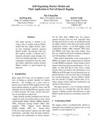
at the apex to less than 1 degree at the toe (Figure 1a).


Fig. 1. (a) Schematic representation of a typical alluvial fan, and (b) representation of a
typical drainage basin
Alluvial fan characterization is concerned with the determination of the role of the fluvial
sediment supply for the evolution of fan deltas. The analysis of the main controlling
factors on past and present fan processes is also of major concern in order to distinguish
between the two dominant sedimentary processes on alluvial fan formation and
evolution: debris flows and stream flows. Crosta & Frattini, (2004), among others, have
worked in two dimensional planimetric area used discriminant analysis methods, while
Giles, (2010), has applied morphometric parameters in order to characterize fan deltas as a
three dimensional sedimentary body. There are studies which have explored on a
probabilistic basis the relationships, between fan morphology, and drainage basin geology

(Melton, 1965; Kostaschuck et al., 1986; Sorisso-Valvo & Sylvester, 1993; Sorisso-Valvo,
1998). Chang & Chao (2006), used back propagation neural networks for occurrence
prediction of debris flows.
In this paper the investigation focuses on two different physiographic features, which are
recent depositional landforms (alluvial fans) in a microrelief scale, and older landforms of
drainage basin areas in a mesorelief scale (Figure 1b). In both cases landform
characterization, is manipulated through the technology of self organising maps (SOMs).
Unsupervised and supervised learning artificial neural networks were developed, to map
spatial continuum among linebased and surface terrain elements. SOM was also applied
as a clustering tool for alluvial fan classification according to dominant formation
processes.
2. Method used
2.1 Self organising maps
Kohonen's self-organizing maps (SOM) (Kohonen, 1995), is one of the most popular
unsupervised neural networks for clustering and vector quantization. It is also a powerful
275
Using Self Organising Maps in Applied Geomorphology
Self Organizing Maps - Applications and Novel Algorithm Design
276
visualization tool that can project complex relationships in a high dimensional input space
onto a low dimensional (usually 2D grid). It is based on neurobiological establishments that
the brain uses for spatial mapping to model complex data structures internally: different
sensory inputs (motor, visual, auditory, etc.) are mapped onto corresponding areas of the
cerebral cortex in an ordered form, known as topographic map. The principal goal of a SOM
is to transform an incoming signal pattern of arbitrary dimension n into a low dimensional
discrete map. The SOM network architecture consists of nodes or neurons arranged on 1-D
or usually 2-D lattices (Fig. 2). Higher dimensional maps are also possible, but not so
common.

Fig. 2. Examples of 1-D, 2-D Orthogonal and 2-D Hexagonal Lattices
Each neuron has a d dimensional weight vector (prototype or codebook vector) where d is
equal to the dimension of the input vectors. The neurons are connected to adjacent neurons
by a neighborhood relation, which dictates the topology, or structure, of the map.
The SOM is trained iteratively. In each training step a sample vector x from the input data
set is chosen randomly and the distance between x and all the weight vectors of the SOM, is
calculated by using an Euclidean distance measure. The neuron with the weight vector
which is closest to the input vector x is called the Best Matching Unit (BMU). The distance
between x and weight vectors is computed using the equation below:

^
`
min
cii
xm x m 
(1)
where ||.|| is the distance measure, typically Euclidean distance. After finding the BMU,
the weight vectors of the SOM are updated so that the BMU is moved closer to the input
vector in the input space. The topological neighbors of the BMU are treated similarly. The
update rule for the weight vector of i is

      
1
iici i
xt mt ath t xt mt  ª  º
¬¼
(2)
where x(t) is an input vector which is randomly drawn from the input data set, a(t)
function is the learning rate and t denotes time. A Gaussian function h

ci
(t) is the
neighborhood kernel around the winner unit m
c
, and a decreasing function of the distance
between the i
th
and c
th
nodes on the map grid. This regression is usually reiterated over
the available samples.
All the connection weights are initialized with small random values. A sequence of input
patterns (vectors) is randomly presented to the network (neuronal map) and is compared to
weights (vectors) “stored” at its node. Where inputs match closest to the node weights, that
276
Self Organizing Maps - Applications and Novel Algorithm Design
Using Self Organising Maps in Applied Geomorphology
277
area of the map is selectively optimized, and its weights are updated so as to reproduce
the input probability distribution as closely as possible. The weights self-organize in the
sense that neighboring neurons respond to neighboring inputs (topology which preserves
mapping of the input space to the neurons of the map) and tend toward asymptotic
values that quantize the input space in an optimal way. Using the Euclidean distance
metric, the SOM algorithm performs a Voronoi tessellation of the input space (Kohonen,
1995) and the asymptotic weight vectors can then be considered as a catalogue of
prototypes, with each such prototype representing all data from its corresponding
Voronoi cell.
2.2 SOM visualization and analysis
The goal of visualization is to present large amounts of information in order to give a
qualitative idea of the properties of the data. One of the problems of visualization of

multidimensional information is that the number of properties that need to be visualized is
higher than the number of usable visual dimensions.
SOM Toolbox (Vesanto, 1999; Vesanto & Alboniemi, 2000), a free function library package
for MATLAB, offers a solution to use a number of visualizations linked together so that one
can immediately identify the same object from the different visualizations (Buza et al., 1991).
When several visualizations are linked in the same manner, scanning through them is very
efficient because they are interpreted in a similar way. There is a variety of methods to
visualize the SOM. An initial idea of the number of clusters in the SOM as well as their
spatial relationships is usually acquired through visual inspection of the map. The most
widely used methods for visualizing the cluster structure of the SOM are distance matrix
techniques, especially the unified distance matrix (U-matrix). The U-matrix visualizes
distances between prototype vectors and neighboring map units and thus shows the cluster
structure of the map. Samples within the same unit will be the most similar according to the
variables considered, while samples very different from each other are expected to be
distant in the map. The visualization of the component planes help to explain the results of
the training. Each component plane shows the values of one variable in each map unit.
Simple inspection of the component layers provides an insight to the distribution of the
values of the variables. Comparing component planes one can reveal correlations between
variables.
Another visualization method offered by SOM is displaying the number of hits in each map
unit. Training of the SOM, positions interpolating map units between clusters and thus
obscures cluster borders. The Voronoi sets of such map units have very few samples (“hits”)
or may even be empty. This information is utilized in clustering the SOM by using zero-hit
units to indicate cluster borders.
The most informative visualizations of all offered by SOM are simple scatter plots and
histograms of all variables. Original data points (dots) are plot in the upper triangle,
though map prototype values (net) are plot on the lower triangle. Histograms of main
parameters are plot on the diagonal. These visualizations reveal quite a lot of information,
distributions of single and pairs of variables both in the data (upper triangle) and in the
trained map (lower triangle). They visualize the parameters in pairs in order to enhance

their correlations. A scatter diagram can extend this notion to the multiple pairs of
variables.
277
Using Self Organising Maps in Applied Geomorphology
Self Organizing Maps - Applications and Novel Algorithm Design
278
3. Study area
The case study area is located on the northwestern part of the tectonically active Gulf of
Corinth which is an asymmetric graben in central Greece trending NW-SE across the
Hellenic mountain range, approximately perpendicular to the structure of Hellenides
(Brooks & Ferentinos, 1984; Armijo et al., 1996). The western part of the gulf, where the
study area is located, is presently the most active with geodetic extension rates reaching up
to 14-16 mm/yr (Briole et al., 2000). The main depositional landforms along this part of the
gulf’s coastline are coastal alluvial fans (also named fan deltas) which have developed in
front of the mouths of fourteen mountainous streams and torrents. Alluvial fan
development within the study area is the result of the combination of suitable conditions for
fan delta formation during the Late Holocene. Their evolution and geomorphological
configuration is affected by the tectonic regime of the area (expressed mainly by
submergence during the Quaternary), weathering and erosional surface processes
throughout the corresponding drainage basins, mass movement (especially debris flows),
and the stabilization of the eustatic sea-level rise about 6,000 years ago (Lambeck, 1996).


Fig. 3. Simplified lithological map of the study area
Apart from the classification of microscale landforms, such as the above mentioned coastal
alluvial fans, this study also focuses on mesoscale landforms characterization. This attempt
concerns the hydrological basin areas of the streams of (from west to east) Varia, Skala,
Tranorema, Marathias, Sergoula, Vogeri, Hurous, Douvias, Gorgorema, Ag. Spiridon,
Linovrocho, Mara, Stournarorema and Eratini, focusing on the catchments of Varia and
278

Self Organizing Maps - Applications and Novel Algorithm Design
Using Self Organising Maps in Applied Geomorphology
279
Skala streams. Landforms distribution within the studied drainage basins are mainly
controlled by the bedrock lithology. Therefore, it is important to outline the geology of the
area. The basic structural pattern of the broader area of the drainage basins was established
during the Alpine folding. The drainage basins are dominated by geological formations of
the geotectonic zones of Parnassos–Ghiona, Olonos-Pindos and Ionian and the Transitional
zone between those of Parnassos–Ghiona and Olonos-Pindos. The easternmost basins
(Eratini and part of Stournarorema) are made up of Tithonian to Senonian limestones of the
Parnassos–Ghiona zone and the Transitional Sedimentary Series (limestones of Upper
Triassic to Paleocene age and sandstones and shales of the Paleocene–Eocene flysch). The
majority of the catchments consist of the Olonos–Pindos zone formations which are
represented by platy limestones of Jurassic-Senonian age and Upper Cretaceous - Eocene
flysch lithological sequences (mainly sandstones and shales). Part of the westernmost Varia
drainage system drains flysch formations (mainly marls, sandstones and conglomerates) of
the Ionian zone. A simplified lithological map of the catchments is presented in Fig3.
Tectonically the area is affected by an older NW-SE trending fault system, contemporaneous
to the Alpine folding and a younger one having an almost E-W direction with the active
normal fault of Marathias (Gallousi & Koukouvelas, 2007) and normal faults located in the
broader area of Trizonia Island being the most significant.
4. Application of SOM in landform characterization - Input variables and data
preparation
This research is based on quantitative and qualitative data depicting the morphology and
morphometry of fans and their drainage basins. These data derived from field-work, SRTM
DEM data and topographic and geological maps at various scales. The correlation between
geomorphological features (expressed by morphometric parameters) of the drainage basins
and features of their fan deltas was detected, in order to determine the role of the fluvial
sediment supply for the evolution of the fan deltas.
A simplified lithological map of the area was constructed from the geological maps of

Greece at the scale of 1:50,000 obtained from the Institute of Geology and Mineral
Exploration of Greece (I.G.M.E.). The lithological units cropping out in the basins area were
grouped in three categories including limestones, flysch formations (sandstones, shales and
conglomerates) and unconsolidated sediments. The area cover occupied from each one of
the three main lithological types in the area of each basin was also estimated.
The identification and delineation of the fans was based upon field observations, aerial
photo interpretation and geological maps of the surficial geology of the area at the scale of
1:50,000 (Paraschoudis, 1977; Loftus & Tsoflias, 1971). Detailed topographic diagrams at the
scale of 1:5.000, were used for the calculation of the morphometric parameters of the fan
deltas. All topographic maps were obtained from the Hellenic Military Geographical
Service (H.M.G.S). The elevation of the fan apex was measured by altimeter or GPS for
most of the studied fans. All measurements and calculations of the morphometric
parameters were performed using Geographical Information System (GIS) functions. The
morphometric variables obtained for each fan and its corresponding drainage basin are
described in Table 1.
Table 2 presents the values of the (fifteen) morhometric parameters measured and estimated
for the coastal alluvial fans and their drainage basins.
279
Using Self Organising Maps in Applied Geomorphology
Self Organizing Maps - Applications and Novel Algorithm Design
280
Drainage basin morphometric parameters
Morphometric Parameter Symbol Explanation
1 Drainage basin area (A
b
)
The total planimetric area of the basin above
the fan a
p
ex, measured in km

2
.
2 Basin crest (C
b
)
The maximum elevation of the draina
g
e basin
g
iven in m.
3
Perimeter of the draina
g
e
basi
n

(P
b
)
The len
g
th of the basin border measured in
km.
4
Total len
g
th of the
channels within the
draina

g
e basi
n
(L
c
) Measured in km.
5
Total length of 20 m
contour lines within the
drainage basin
(ƴL
c
) Measured in km.
6 Basin relief (R
b
)
Corresponds to the vertical difference between
the basin crest and the elevation of fan apex,
g
iven in m.
7
Melton’ s ruggedness
number
(M)
An index of basin ru
gg
edness (Melton, 1965,
Church and Mark, 1980) calculated by the
following formula:
M=R

b
A
b
-0.5
8 Drainage basin slope (S
b
)
Obtained usin
g
the followin
g
equation :
S
b
=eƴL
c
/A
b

e is the equidistance (20m for the maps that
were used in this stud
y)
.
9 Drainage basin circularity (Cir
b
)
It is given by the equation:
Cir
b
=4ǑA

b
/P
b
2
and expresses the shape of the
basin.
10 Drainage basin density (D
b
)
The ratio of the total len
g
th of the channels to
the total area of the basin.
Fan delta morphometric parameters
11 Fan area (A
f
)
The total planimetric area of each fan,
measured in km
2
.
12 Fan length (L
f
)
The distance between the toe (coastline for
most of the fans) and apex of the fan,
measured in m.
13 Fan apex (Ap
f
) The elevation of the apex of the fan in m.

14 Fan slope (S
f
)
The mean
g
radient measured alon
g
the axial
p
art of the fan.
15 Fan concavity (C
f
)
An index of concavit
y
alon
g
the fan axis defined
as the ratio of a to b, where a is the elevation
difference between the fan axis profile and the
midpoint of the straight line joining the fan apex
and toe, and b is the elevation difference between
the fan toe and mid
p
oint.
Table 1. Definition of drainage and fan delta morphometric parameters
280
Self Organizing Maps - Applications and Novel Algorithm Design
Using Self Organising Maps in Applied Geomorphology
281

Stream/fan
name
A
b
C
b
P
b
L
c
ƴL
c
R
b
M S
b
Cir
b
D
b
A
f
L
f
Ap
f
S
f

C
f

1 Varia 27.5 1420 26.5 85.9 592.2 1376 0.26 0.43 0.49 3.13 4.2 2.6 44 0.017 1.10
2 Skala 28.2 1469 25.6 80.6 785.1 1375 0.26 0.56 0.54 2.86 4.2 2.9 94 0.033 1.29
3 Tranorema 30.3 1540 26.4 112.4 798.7 1452 0.26 0.53 0.55 3.70 1.6 2.1 88 0.042 1.05
4 Marathias 2.3 880 6.8 6.6 52.8 788 0.52 0.46 0.63 2.87 0.4 0.6 92 0.157 1.28
5 Sergoula 18.4 1510 19.7 59.7 569.8 1456 0.34 0.62 0.60 3.24 0.5 1.2 54 0.046 1.16
6 Vogeni 2.4 1035 7.9 5.6 63.7 817 0.53 0.53 0.49 2.34 0.7 1.3 218 0.167 1.38
7 Hurous 6.8 1270 11.6 23.2 158.6 1054 0.41 0.47 0.63 3.43 2.7 2.8 216 0.077 1.63
8 Douvias 6.8 1361 10.6 23.6 190.3 1269 0.49 0.56 0.77 3.46 0.6 1.6 92 0.059 1.42
9 Gorgorema 2.5 1060 7.3 6.2 67.7 1012 0.64 0.55 0.59 2.52 0.1 0.6 48 0.082 1.18
10
Ag.
Spiridon 1.0 585 4.4 3.5 32.2 515 0.50 0.62 0.69 3.39 0.1 0.7 70 0.095 1.33
11 Linovrocho 3.6 1020 8.6 11.3 86.4 926 0.49 0.47 0.62 3.09 0.3 1.2 94 0.080 1.04
12 Mara 2.1 711 6.8 7.8 51.4 651 0.45 0.50 0.57 3.76 0.2 0.8 60 0.076 1.14
13
Stournaro-
rema 47.1 1360 31.5 142.1 1236.0 1268 0.18 0.53 0.60 3.02 4.7 4.5 92 0.021 1.56
14 Eratini 3.4 1004 8.8 8.6 77.7 974 0.53 0.46 0.55 2.55 0.3 0.7 30 0.044 1.30
Table 2. Values of the measured morphometric parameters for the 14 alluvial fans and their
drainage basins
Two more qualitative parameters were studied, the existence or not of a well developed
channel in fan area (R), and the geological formation that prevails in the basin area (GEO).
Channel occurrence or absence was coded in a binary condition, whereas geological
formation prevalence was coded according to relative erodibility.

Nr Stream/fan name GEO R Nr Stream/fan name GEO R
1 Varia flysch 1 8 Douvias limestone 1

2 Skala limestone 1 9 Gorgorema flysch 1
3 Tranorema flysch 0 10 Ag. Spiridon flysch 0
4 Marathias limestone 1 11 Linovrocho flysch 1
5 Sergoula limestone 0 12 Mara flysch 1
6 Vogeni limestone 0 13 Stournarorema flysch 1
7 Hurous flysch 1 14 Eratini limestone 0
Table 3. Values of the studied categorical parameters for the 14 alluvial fans and their
drainage basins
281
Using Self Organising Maps in Applied Geomorphology
Self Organizing Maps - Applications and Novel Algorithm Design
282
Satellite derived DEMs were also used for digital representation of the surface elevation.
The source were global elevation data sets from the Shuttle Radar Topography Mission
(SRTM)/SIR-C band data, (with 1 arc second and 3 arc seconds) released from (NASA). In
this study, two DEMs were re-projected to Universal Transverse Mercator (UTM) grid,
Datum WGS84, with 250m and 90m spacing. In the proposed semi-automatic method, it is
necessary to implement algorithms, which identify landforms from quantitative, numerical
attributes of topography. Morphometric analysis of the study area was performed using the
DEM and the first and second derivatives (slope, aspect, curvature, plan and profile
curvature), applying Zevenbergen & Thorne (1987) method. Morphometric feature analysis
and extraction of morphometric parameters are implemented in the open source SAGA GIS
software, version 2.0 (SAGA development team 2004). Routines were applied in order to
perform terrain analysis and produce terrain forms using Peuker & Douglas (1975), method.
This method considers the slope gradients to all lower and higher neighbors for the cell
being processed. For example, if all the surrounding neighbor cells have higher elevations
than the cell being processed, the cell is a pit and vice versa is a peak. If half of the
surrounding cells are lower in elevation and half are higher in elevation, then the cell being
processed is on a hill-slope. The cell being processed is identified as a ridge cell if only one
of the neighboring cells is higher, and, conversely, a channel when only one neighbor cell is

lower. When slope gradients are considered, a hill-slope cell can be further characterized
between a convex or concave hill-slope position. At locations with positive values for slope,
channels have negative cross sectional curvature whereas ridges have positive cross
sectional curvatures. The differentiation to plan hill-slopes is performed by using a
threshold.

Symbol Description
Nr of data samples in
250m DEM spacing of
the whole data set
Nr of data samples in 90m
DEM spacing of the subset
of Varia and Scala basin
-9 Pit 26 113
-7 Channel 825 6,322
-2
Concave break
form valleys
683 5,284
0 Flat 99 1,060
1 Pass 4 371
2
Convex break
form ridges
713 5,441
7 Ridge 805 6,289
9 Peak 17 138
Table 4. Terrain form classification according to Peuker & Douglas method
Sampling procedure for the data set describing the drainage basins and alluvial fan regions,
was performed. A sampling function was applied to the derivatives grids in order to

prepare a matrix of sample vectors. The produced ASCII file was exported to MATLAB in
order to use SOM artificial neural networks. The main geomorphological elements
according to Peuker and Douglas (1975) method, are channels, ridges, convex breaks and
concave breaks and are presented in Table 4. Pits, peaks and passes are not so often in the
study area. The morphometric parameters derived were used as input to SOM. Data
preparation in general is a diverse and difficult issue. It aims to, select variables and data
282
Self Organizing Maps - Applications and Novel Algorithm Design
Using Self Organising Maps in Applied Geomorphology
283
sets to be used for building the model, clean erroneous or uninteresting values from the
data. It also aims to transform the data into a format which the modelling tool can best
utilize and finally normalize the values in order to accomplish a unique scale and avoid
problems of parameter prevalence according to their high values.
The quality of the SOM obtained with each normalization method is evaluated using two
measures as criteria: the quantization error (QE) and the topographic error (TE). QE is the
average distance between each data set data vector and its best mapping unit, and thus,
measures map resolution (Kohonen, 1995). TE is used as a measure of topology
preservation. The map size is also important in the SOM model. If the map is too small, it
might not explain some important differences, but if the map is too large (i.e. the number of
map units is larger than the number of samples), the SOM can be over fitted (Lee & Scholz,
2006). Under the condition that the number of neurons could be close to the number of the
samples, the map size was selected, for each application.
5. Results
5.1 Microscale landform characterization (coastal alluvial fan classification)
The application of the SOM algorithm in the current data set, and the result of the clustering
are presented through the multiple visualization in Fig.4. The examined variables are the
morphometric parameters of the alluvial fans and their corresponding drainage basins,
analytically presented in Tables 1 and 2. The lowest values of QE and TE were obtained
using logistic function which scales all possible values between [0,1]. Batch training took

place in two phases. The initial phase is a robust one and then a second one is fine-tuning
with a smaller neighborhood radius and smaller (learning rate). During rough initial
neighborhood radius and learning rate were large. Gradually the learning rate decreased
and was set to 0.1, and radius was set to 0.5.
Visualization in Fig. 4 consists of 19 hexagonal grids (the U-matrix upper left, along with the
17 component layers and a label map on the lower right). The first map on the upper left
gives a general picture of the cluster tendency of the data set. Warm colors represent the
boundaries of the clusters, though cold colors represent clusters themselves. In this matrix
four clusters are recognized. In Fig.5a and Fig.5c the same vislualization is presented
through hit numbers in Fig. 5a and the post–it labels in Fig. 5c. The hit numbers in the
polygons represent the record number, of the data set that belong to the same neighborhood
(cluster). Through the visual inspection of both Fig.5a and Fig.5c, one corresponds the hit
numbers to the particular record, which is the alluvial fan name. Four clusters were
generated. The records that belong to the same cluster are mapped closer and have the same
color. For example, Marathias and Vogeni belong to the same cluster represented with blue.
The common characteristics of these two fans are visualized through Fig. 4. Using similarity
coloring and position, one can scan through all the parameters and reveal that these two
records mapped in the upper corner of each parameter map have always the same values
represented by similar color.
Except from general clustering tendency, scanning through parameter layers one can
reveal correlation schemes, always following similarity colouring and position. Each
parameter map is accompanied with a legend bar that represents the range values of the
particular parameter. Drainage basin area (A
b
) is correlated with fan area (A
pf
) and fan
length (L
f
).

283
Using Self Organising Maps in Applied Geomorphology
Self Organizing Maps - Applications and Novel Algorithm Design
284

Fig. 4. SOM visualization through U-matrix (top left), and 17 component planes, one for
each parameter examined. The figures are linked by position: in each figure, the hexagon in
a certain position corresponds to the same map unit
Total length of channels (L
c
) within basin area (A
b
), and total length of contours (ƴL
c
) within
the drainage basin are also correlated (see red and yellow circles in Fig. 4). Basin crest (C
b
),
and basin relief (R
b
) are inversely correlated (see green circle in Fig. 4). Melton’s’ ruggedness
number is inversely correlated to fan slope (S
f
), but correlated to channel development in fan
area (see black circles in Fig. 4). The geological formation prevailing to basin area seems to
be inversely correlated to concavity, (i.e. limestone basins have produced less concave fans
compared to the flysch ones). Concavity (C
f
) is also correlated to fan area (A
pf

).
Analysis of each cluster is then carried out to extract rules that best describe each cluster by
comparing with component layers. The rules to model and predict the generation of alluvial
fans, are extracted by mapping the four clusters presented in Fig.5 with the input
morphometric parameters (component planes) in Fig.4. Prior to rules extraction each input
variable is divided in three categories, that is low and high and medium. The threshold value,
which separates each category, is determined from the component planes legend bar in Fig.4.
In the following description, the response of the given data to the map (adding hits number)
for each cluster was calculated as a cluster index value (CIV). The higher the cluster index
value the stronger the cluster and therefore the most important in the data set and the most
representative for the study area.
Cluster 1: Varia, Skala, Sergoula, Stournarorema, Tranorema. The cluster index was
calculated (5). Varia and Tranorema form a subgroup. Stournarorema and Scala form a
second subgroup. This group includes fans formed by streams with well developed
drainage networks and large basins with high values of basin relief. The produced fans are
extensively and relatively gently sloping (with a mean slope of 0.03). Varia, Skala, Sergoula
and Stournarorema fans have a triangular shape and resemble small deltas while Tranorema
has a more semicircular morphology. These fans are intersected by well developed and
clearly defined distributary channels consisting of coarse grained material (pebbles, cobles
284
Self Organizing Maps - Applications and Novel Algorithm Design
Using Self Organising Maps in Applied Geomorphology
285
and few boulders). These are generally aggrading fans with an active prograding area near
the river mouth. The fans of this group are characterized as fluvial dominated.
Cluster 2: Marathias, Vogeni. The cluster index is (2). This second group involves fans
formed by torrents with small drainage basins. They have developed laterally overlaying or
confining fans of the cluster 1. Their shape is conical, they do not present well developed
channels and are also characterized from high fan gradients (mean fan slope reaches 0.4).
Flysch formations prevail in their basin area. According to these features, they seem to be

debris flow dominated. Their formation and evolution is inferred to be highly governed
from the two serious landslides of Marathias and Sergoula, occurred in the study area.
Cluster 3: Gorgorema, Mara, Linovrocho, Ag. Spyridon, Eratini. The cluster index is (5). This
group includes alluvial fans formed by streams of well developed drainage networks with
large basins dominated by the presence of flysch formations. The fans are elongated and
have well developed and clearly defined distributary channels, relatively incised in the most
proximal part of the fan, near the apex, which become indefinite at the lower part near the
coastline. The slope of their surface (mean gradient of 0.08) is higher than the slope of the
cluster 1 fans and lower than those of cluster 2. According to these findings they are
characterized as fluvial dominated with debris flow influences.
Cluster 4: Hurus and Douvias. The cluster index value is (2). The drainage basins of these
two streams have similar features. These two fans are elongated and have well developed
distributary channels, low slope values and high concavity. Their main characteristic is the
large fan area if compared with the catchment area. The anomalously large Hurus torrent
alluvial fan in relation to its drainage basin area is interpreted to be the result of abnormally
high sediment accumulation at the mouth of this torrent. This exceptional accumulation rate
is attributed to reduce of marine processes effectiveness due to the presence of Trisonia
Island in front of the torrent mouth. This island protects the area of the fan resulting in
deposition of the fluvio-torrential material. They are characterised as fluvial dominated fans.


Fig. 5. Different visualizations of the clusters obtained from the classification of the
morphological variables through SOM. (a) Colour code using k-means; (b) Principal
component projection; (c) Label map with the names of the alluvial fans, using k-means. .
The four clusters are indicated through the coloured circles
285
Using Self Organising Maps in Applied Geomorphology
Self Organizing Maps - Applications and Novel Algorithm Design
286
In Table 5 the rules governing each class are described.

Explanation Symbol Group1 Group2 Group3 Group4
Cluster Index
Value CIV 5 2 5 2

fluvial
dominated debris flow
fluvial
dominated
with debris
flow
influences
fluvial
dominated

Varia, Skala,
Sergoula,
Stournarorema,
Tranorema
Marathias,
Vogeni
Ag.
Spyridon,
Mara,
Gorgorema,
Linovrocho,
Eratini
Dounias,
Hurous
Drainage basin area (A

b
) > 15.8 High < 15.8 Low < 15.8 Low Medium
Basin crest (C
b
) > 1160 High < 1160 Low < 1160 Low > 1160 High
Perimeter of the
drainage basin (P
b
) >15.4 High < 15.4 Low < 15.4 Low < 15.4 Low
Total length of the
channels within the
drainage basin (L
c
) > 48.6 High < 48.6 Low < 48.6 Low < 48.6 Low
Total length of 20 m
contour lines within
the drainage basin (ƴL
c
) > 421 High < 421 Low < 421 Low < 421 Low
Basin relief (R
b
) < 437 Low > 437 High > 437 High < 437 Low
Melton’ s
ruggedness number (M) < 0.4 Low > 0.4 High > 0.4 High Medium
Drainage basin
slope (S
b
) Medium to high <0.08 Low <0.08 Low >0.08 High
Drainage basin
circularity (Cirb) <0.60 Low <0.60 Low Medium >0.60 High

Drainage basin
density (D
b
) > 3.05 High < 3.05 Low Medium > 3.05 High
Fan area (A
f
) >1.97 High <1.97 Low <1.97 Low Medium
Fan length (L
f
) <1.93 High >1.93 Low >1.93 Low >1.93 Medium
Fan apex (Ap
f
) not clear > 100 High < 100 Low > 100 High
Fan slope (S
f
) < 0.03 Low > 0.03 High Medium < 0.03 Low
Fan concavity (C
f
) not clear >1.28 High Medium >1.28 High
286
Self Organizing Maps - Applications and Novel Algorithm Design
Using Self Organising Maps in Applied Geomorphology
287
Well developped
channels R Yes No Yes Yes
Prevailing
geological
formation in basin
area Geo Limestone Flysch Flysch Limestone
Table 5. Clusters originating from SOM classification

5.2 Mesoscale landform characterization using unsupervised SOM
The systematic classification of landforms, their components, and associations, as well as
their regional structure is one prerequisite for understanding geomorphic systems on
different spatial and temporal scales (Dikau & Schmidt, 1999). The aim is to locate any
correlation schemes between first and second derivatives describing the basin areas and
alluvial fan regions, and examine clustering tendency of the data to certain line or surface
morphometric features, (i.e. channels, ridges, planar surfaces). The data set comprised 3222
records, from a 250m spacing DEM, covering the whole study area (i.e. fourteen drainage
basins and corresponding alluvial fans).
In order to assess the optimum SOM, 11 SOMs were developed. Learning of SOM was
performed with random initial weighs of the map units. The initial radius was set to 3 and
the final radius to 1. The initial learning rate was set to 0.5 and the final to 0.05.
Experimenting towards SOM optimization the size of the map progressively augmented
from 70 to 300, with a decreasing (QE) from 0.37 to 0.25. The optimum architecture was built
through trial and error procedure. The SOM which gave the best map had QE 0.111 after
1000 epochs (Fig. 6). The optimum architecture was used in 10 more trials with random
initial weights, so as to test the influence, on (QE). According to the findings of this study,
there was no influence, which is probably attributed to the long time of training. That is,
initial random weight values are being trained and Euclidian distances between input data
vectors and best matching units decrease and reach the minimum value and become stable.


Fig. 6. Effect of number of epochs on average quantization error
287
Using Self Organising Maps in Applied Geomorphology
Self Organizing Maps - Applications and Novel Algorithm Design
288


a

b
Fig. 7. (a) SOM visualization through U-matrix (top left), and 6 component planes, one for
each parameter examined (b) from left to right, through, Davis - Bouldin validity index
versus cluster number, colour coding, and clustering using k-means (upper left (1) counting
clockwise, (9) in the centre
9 Clusters
288
Self Organizing Maps - Applications and Novel Algorithm Design
Using Self Organising Maps in Applied Geomorphology
289

Fig. 8. SOM visualization through scatter diagrams of studied morphometric parameters
The next step is the analysis, interpretation and labeling of the map units as morphometric
features. Correlation between slope and elevation, curvature and plan curvature is
displayed through U-matrix (Fig. 7) and scatter diagrams (Fig. 8). Profile curvature is
inversely correlated to plan curvature. No clear correlation on aspect and the other
derivatives is portrayed.
U-matrix shows no clear separation between clusters, but using k-means algorithm and Davis
– Bouldin (1979) index (Fig. 7b), it seems that 9 existing clusters correspond to different terrain
forms. From the component planes, it can be seen that the features differentiating the clusters
are the following presented in Table 7. In this table, the categorized map units and the
corresponding morphometric features are summarized. For example ridges in the study area
are represented with clusters 1,2,7 but with different slope and elevation conditions. This
feature corresponds to both steeper and slopes representing an approximately flat area.
Cluster 9 corresponds to flat area, possibly planation areas, in higher elevation almost flat
terrain. Cluster 3 and 8 correspond to channels, with different slope conditions.
The black boxes plotted in Fig.8 refer to convex ridges, and the cyan boxes to concave
channels. In order to hunt correlations between parameters, one should scan through the

scatter diagrams in the lower triangle (resulting after training) where both data and map
units are plot. According to SOM training, channels (negative concavities) are recognized
and constitute two subgroups from low to steep slopes. Convex ridges are also recognized
separated in classes from moderate to steep slopes. Planar surfaces are also recognized and
differentiated according to slope angle. It is evident in Fig.8, that planar surfaces of gentle to
steep slopes exist, in the study area.
289
Using Self Organising Maps in Applied Geomorphology
Self Organizing Maps - Applications and Novel Algorithm Design
290
Class Morphometric
element
Slope (ͼ)Elevation
(m)
Curvature Profile
curvature
Plan
curvature
Aspect
Cluster 1 Ridge
Medium
(16)
Medium to
High 580
to 1070
+ 0 + E to SE
Cluster 2 Ridge
Medium
to High >
(16)

High > 750 + 0 + W
Cluster 3 Channel
High >
(23)
Medium -
High > 560
- + - W
Cluster 4 Planar
Medium
to high
High > 750 0 + 0 E to N
Cluster 5 Planar
Low to
Medium
Low < 560 0 + 0 E to NE
Cluster 6 Chanel Very Low Low - + - E
Cluster 7 Ridge Low Low + - + S to SW
Cluster 8 Chanel High Low - + - W
Cluster 9 Planar Low High 0 0 0 NE to E
Table 7. Clusters originating from SOM
5.3 Mesoscale landform characterization using supervised SOM
SOM algorithm was proposed, as an alternative procedure for terrain analysis to Peuker and
Douglass method. SOM training was performed with a subset of the DEM, referring to Varia
and Scala drainage basins (see Fig.3). Six morphometric parameters were used, as input and
a two-dimensional output of 3,000 neurons. Sampling procedure for the data set describing
the drainage basins was performed. A sampling function was applied to the derivatives
grids in order to prepare a matrix of sample vectors. The sampling was performed to the
DEM and DEM derivatives, at 90m spacing. Problems handling memory had to be faced,
this is why a small subset of the training DEM was used. The produced ASCII file was
exported to MATLAB in order to use SOM unsupervised neural networks. The data set is

presented in Table 4. The data dimensions was 25,024 x 6.
At the beginning of the learning procedure, neurons in the SOM were distributed randomly.
The BMUs (final classes) with minimum average (QE) 0.135 were extracted. The number of map
units was finally set to 3,000. Turning the SOM into a supervised classifier the final error was
30%. In table 8 the results of the applied normalizations are displayed. The error of supervised
clustering is also presented. “HistD” normalization gave the best results, after 1,000 iterations.

Normalization method QE TE error
histC 0.182 0.040 36.8
Var 0.40 0.045 35.4
Log 0.198 0.036 28.4
Logistic 0.34 0.054 33.61
Range 0.180 0.050 41.52
histD 0.210 0.033 27.92
Table 8. Normalization methods, and calculated QE and TE, for supervised clustering
290
Self Organizing Maps - Applications and Novel Algorithm Design
Using Self Organising Maps in Applied Geomorphology
291



Fig. 9. Outcome of Peuker and Douglas classification
The results of the supervised clustering are presented in Fig. 10. The results illustrate a
very clear distinction between the disparate morphometric features. Line-based and
planar features were mainly recognized. A rather good network of ridges and channels
with different slope classes is revealed. Compared to the outcome of classic morphometric
analysis in Fig. 9 the outcome we get through SOM seems more compact, with a very
good representation of crest lines. According to Peuker and Douglas method about 41% of
the area are concave and convex breaks, 27 % are channels and 28% are ridges. As

expected point- based features such as peaks, passes and pits cover only 4% of the study
area. This is probably attributed to the fact that point based features are comparatively
rare.



Fig. 10. Outcome of SOM clustering
291
Using Self Organising Maps in Applied Geomorphology
Self Organizing Maps - Applications and Novel Algorithm Design
292
6. Discussion
Given that geomorphological mapping is the basis for terrain assessment, a
geomorphological map was constructed, to validate the results of the SOM drainage basin
landscape mesoscale classification, for the catchments of Varia and Skala streams which are
the two westernmost among the studied basins (Fig.11). Geomorphological mapping was
performed using a 1:50,000 base topographic map through fieldwork, and aerial photo
interpretation taking also into account previous geological maps.


Fig. 11. Geomorphological map of the Varia and Skala streams and drainage basin areas,
bedrock lithology is derived by the geological maps of (IGME) and field observations
The purpose of the mapping, which was its comparison with the SOM derived classification
map, was the main criterion for the selection of the scale of the map. The scale is critical for
effective information delivery. The final map provides information on the distribution of
geological formations while landforms identifying landscape features created by surface
processes were recorded combining field inspection with maps and aerial photo
292
Self Organizing Maps - Applications and Novel Algorithm Design
Using Self Organising Maps in Applied Geomorphology

293
interpretation. These landforms which include erosional planation surfaces ranging in
elevation from 500 m to 1,000m, stream channels and valleys of various shape, knickpoints,
abrupt slope breaks, gentler slope changes, ridges and crests, alluvial fans and cones, intense
channel downcutting, provide information on earth surface form processes.
Comparative observation of the geomorphological map, Peuker and Douglas classification,
and the SOM clustering reveals information on the accuracy of the landscape
characterization approach through SOM. Both methods identified stream channels of the
drainage networks with very accurately. The more well developed high order channels like
those of the main streams of the networks were better detected and recognized using SOM.
Additionally, SOM identified correctly ridges and drainage divides providing an ideal
method for drawing drainage basins borders. On the other hand landforms like erosional
planation surfaces or knickpoints (discrete negative steps in the longitudinal profile of a
river), are not identifiable on the SOM clustering.
In terms of evaluation results, Peuker and Douglas method and SOM, were compared, with
an oblique view, overlaying contour lines (Figure 12). SOM is much closer to the
geomorphological mapping, approach, and has much more potential for identification of
non-point morphometric features than Peuker and Douglas method. The overall pattern of
channels, ridges and planes is similar in both methods, but the SOM results are more
concrete and seem to resemble to the classification of the geomorphological mapping, which
recognizes unique landforms. Furthermore, the SOM capability of identifying crest lines on
mountain ranges is also important. Last, the SOM method does not rely on curvature and
slope tolerance values. In this method, the slope parameter, elevation and aspect, are
important in characterizing classes, rather than just being a threshold to separate horizontal
surfaces from sloping surfaces. Using the whole potential of the slope parameter in
extracting features that are more informative is one of the advantages of the SOM.
Concerning the accuracy of the alluvial fan classification utilizing SOM it is obvious that this
approach provides one of the best methods to characterize alluvial fans considering the
correlation between alluvial fans and geomorphometric characteristics and quantitative
morphometric indices of their corresponding drainage basins.

Fig. 12. Classification results (a) Terrain analysis according to SOM clustering, (b) Terrain
analysis according to Peuker and Douglas
293
Using Self Organising Maps in Applied Geomorphology