Sustainable Wireless Sensor Networks Part 8 doc

Sustainable Wireless Sensor Networks236
became negligible because amortized across a long epoch. This reinforces our choice in
using a slow mobility regime.
After determining the Base Stations placement strategy, we can further prolong network
lifetime by instructing Cluster heads to efficiently forward the data to the destination.
Hence, at the beginning of each round and after it is located in its new position, each Base
Station has to compute the routing scheme that will manage in an energy efficient manner
the inter Cluster Heads communication within its corresponding sub-network.


5. Inter-Cluster Head communication
As discussed at the beginning of this chapter, Cluster Heads that are in critical positions run
out of energy first. Hence, to further extend the network lifetime, it is necessary to delay as
much as possible the first Cluster Heads death.
For small-scale non-clustered WSNs, we proposed in a previous work (Slama et al., 2006) an
approach that defines an optimal multi-hop routing. It dynamically distributes flows
proportionally to the residual energy available at each node leading to a maximum network
lifetime.
The routing scheme is modelled as an optimization algorithm and is computed at the Base
Station. Its resolution results in a routing matrix that defines for each node to which of its
neighbors it has to send data.
In this section, we propose to extend this approach to two-tiered WSN architectures. In
addition to the residual energy at each Cluster Heads, we introduce a new constraint that
reflects Cluster Head energy consumption related to its intra-cluster activities (i.e. the first
role of Cluster Heads). The idea is to alleviate, from relaying activities (i.e. the second role of
Cluster Heads), Cluster Heads requiring higher energy for managing their clusters.
On the other hand, inside each cluster, Sensing Nodes have to provide the information
required by the end application. They should be organized such that the QoS is satisfied
with minimum cost. Different techniques can be used to achieve this goal. For instance,
sensors can be autonomous and self organized (Rabiner, Heizelman et al., 2002, Chatterjee et
al., 2002). Another approach is to use a relative central mechanism (e.g. scheduling

mechanism) that can take the appropriate decisions on behalf of the Sensing Nodes. For
instance, we can consider that within each cluster, one or more Sensing Nodes may be used
at any time to provide data to the application, but only certain subsets of available sensors
may satisfy channel bandwidth and/or application quality of service constraints (Perillo &
Heinzelman, 2003). In this work, we decide to adapt the scheduling mechanism, initially
proposed in (Perillo & Heinzelman, 2003) for a flat topological WSNs, to manage
communications inside the clusters. This scheduler determines which sensor sets should be
used and for how long time so that the lifetime of the cluster is maximized while the
necessary quality of service expected from this cluster is always maintained at the
application. In addition, Sensing Nodes providing redundant information can be turned off
which contributes in energy saving and reduces data flows. Used within each cluster and
according to the performance evaluation given in (Perillo & Heinzelman, 2003), this
mechanism optimizes individual clusters lifetimes.
In order to achieve a global routing optimization , the inter-Cluster Heads communication
approach that we propose should, in addition, take into account these individual clusters
lifetimes, as the more a cluster lasts, the more its Cluster Heads requires energy for its
management (e.g. reception, data processing and fusion, …).
This inter-Cluster Heads communication approach is modeled within each sub-network as
an optimization problem. It is then processed in a centralized manner at the Base Station of
each sub-network independently but simultanously. It takes into account the current status
and topology of the sub-network and results in a routing matrix that defines the inter-
Cluster Heads flows within this sub-network such that the minimum Cluster Head lifetime
is optimized.
The inter-Cluster Heads communication approach construction and its details are presented
in the following sections.

5.1 Model and Notations
Let’s consider
N
b

Base Stations to be deployed in the network. We note a Base Station k by
b
k
, k = 1 to
N
b
. The network graph G is then partitioned into
N
b
equivalent sub-graphs. We
consider (H
1
, H
2
, …,
H
N
b
) the connected partition of G.
Then, each sub-network k corresponding to H
k
contains one single mobile Base Station b
k

and
N
k
CH
Cluster Heads, k = 1 to
N

b
,
NN
k
CH
k


.
We assume that each sub-network k is modeled as a connected sub-graph G
k
(H
k
, A
k
), k = 1 to
N
b
. H
k
is then the set of Cluster Heads belonging to the sub-network k, H
k
= {CH
k,i
, i = 1 to
N
k
CH
} and A
k

the set of the undirected links (CH
k,i
, CH
k,j
) where CH
k,i
and CH
k,j
are two Cluster
Heads of H
k
.
Let L
k,i
be the set of Cluster Heads neighbors of Cluster Head CH
k,i
in the sub-network k. L
k,i

is composed of all Cluster Heads of H
k
that can be reached by CH
k,i
. All links are assumed to
be bidirectional.
We remind that if a Cluster Head belongs to a sub-network than its corresponding Cluster
belongs to this sub-network as well. We will note by
C
k,i
the Cluster of Sensing Nodes

corresponding to the Cluster Head CH
k,i
and then belonging to sub-network k, i = 1 to
N
k
CH

and k = 1 to
N
b
.
Each cluster
C
k,i
contains N
k,i
S
Sensing Nodes. We will refer to the complete set of Sensing
Nodes within a cluster
C
k,i
as
S
k,i
 S
k,il
,l  1 N
k,i
S





.
We remind that all Sensing Nodes in Cluster
C
k,i
can communicate directly with their
Cluster Head CH
k,i
and that all Cluster Heads CH
k,i
belonging to sub-network k have to
forward the gathered data to the Base Station b
k
deployed within this same sub-network.
Also, Cluster Heads belonging to one sub-network cannot communicate with Cluster Heads
belonging to another sub-network.
We finally assume that
E
k,il
S
and
E
k,i
CH

are the initial energies of Sensing Node
S
k,il

and
Cluster Head CH
k,i
respectively. In table 1, we list all symbols used in this chapter.
Topology Control and Routing in Large Scale WSNs 237
became negligible because amortized across a long epoch. This reinforces our choice in
using a slow mobility regime.
After determining the Base Stations placement strategy, we can further prolong network
lifetime by instructing Cluster heads to efficiently forward the data to the destination.
Hence, at the beginning of each round and after it is located in its new position, each Base
Station has to compute the routing scheme that will manage in an energy efficient manner
the inter Cluster Heads communication within its corresponding sub-network.


5. Inter-Cluster Head communication
As discussed at the beginning of this chapter, Cluster Heads that are in critical positions run
out of energy first. Hence, to further extend the network lifetime, it is necessary to delay as
much as possible the first Cluster Heads death.
For small-scale non-clustered WSNs, we proposed in a previous work (Slama et al., 2006) an
approach that defines an optimal multi-hop routing. It dynamically distributes flows
proportionally to the residual energy available at each node leading to a maximum network
lifetime.
The routing scheme is modelled as an optimization algorithm and is computed at the Base
Station. Its resolution results in a routing matrix that defines for each node to which of its
neighbors it has to send data.
In this section, we propose to extend this approach to two-tiered WSN architectures. In
addition to the residual energy at each Cluster Heads, we introduce a new constraint that
reflects Cluster Head energy consumption related to its intra-cluster activities (i.e. the first
role of Cluster Heads). The idea is to alleviate, from relaying activities (i.e. the second role of
Cluster Heads), Cluster Heads requiring higher energy for managing their clusters.

On the other hand, inside each cluster, Sensing Nodes have to provide the information
required by the end application. They should be organized such that the QoS is satisfied
with minimum cost. Different techniques can be used to achieve this goal. For instance,
sensors can be autonomous and self organized (Rabiner, Heizelman et al., 2002, Chatterjee et
al., 2002). Another approach is to use a relative central mechanism (e.g. scheduling
mechanism) that can take the appropriate decisions on behalf of the Sensing Nodes. For
instance, we can consider that within each cluster, one or more Sensing Nodes may be used
at any time to provide data to the application, but only certain subsets of available sensors
may satisfy channel bandwidth and/or application quality of service constraints (Perillo &
Heinzelman, 2003). In this work, we decide to adapt the scheduling mechanism, initially
proposed in (Perillo & Heinzelman, 2003) for a flat topological WSNs, to manage
communications inside the clusters. This scheduler determines which sensor sets should be
used and for how long time so that the lifetime of the cluster is maximized while the
necessary quality of service expected from this cluster is always maintained at the
application. In addition, Sensing Nodes providing redundant information can be turned off
which contributes in energy saving and reduces data flows. Used within each cluster and
according to the performance evaluation given in (Perillo & Heinzelman, 2003), this
mechanism optimizes individual clusters lifetimes.
In order to achieve a global routing optimization , the inter-Cluster Heads communication
approach that we propose should, in addition, take into account these individual clusters
lifetimes, as the more a cluster lasts, the more its Cluster Heads requires energy for its
management (e.g. reception, data processing and fusion, …).
This inter-Cluster Heads communication approach is modeled within each sub-network as
an optimization problem. It is then processed in a centralized manner at the Base Station of
each sub-network independently but simultanously. It takes into account the current status
and topology of the sub-network and results in a routing matrix that defines the inter-
Cluster Heads flows within this sub-network such that the minimum Cluster Head lifetime
is optimized.
The inter-Cluster Heads communication approach construction and its details are presented
in the following sections.

5.1 Model and Notations
Let’s consider
N
b
Base Stations to be deployed in the network. We note a Base Station k by
b
k
, k = 1 to
N
b
. The network graph G is then partitioned into
N
b
equivalent sub-graphs. We
consider (H
1
, H
2
, …,
H
N
b
) the connected partition of G.
Then, each sub-network k corresponding to H
k
contains one single mobile Base Station b
k

and

N
k
CH
Cluster Heads, k = 1 to
N
b
,
NN
k
CH
k


.
We assume that each sub-network k is modeled as a connected sub-graph G
k
(H
k
, A
k
), k = 1 to
N
b
. H
k
is then the set of Cluster Heads belonging to the sub-network k, H
k
= {CH
k,i
, i = 1 to

N
k
CH
} and A
k
the set of the undirected links (CH
k,i
, CH
k,j
) where CH
k,i
and CH
k,j
are two Cluster
Heads of H
k
.
Let L
k,i
be the set of Cluster Heads neighbors of Cluster Head CH
k,i
in the sub-network k. L
k,i

is composed of all Cluster Heads of H
k
that can be reached by CH
k,i
. All links are assumed to
be bidirectional.

We remind that if a Cluster Head belongs to a sub-network than its corresponding Cluster
belongs to this sub-network as well. We will note by
C
k,i
the Cluster of Sensing Nodes
corresponding to the Cluster Head CH
k,i
and then belonging to sub-network k, i = 1 to
N
k
CH

and k = 1 to
N
b
.
Each cluster
C
k,i
contains N
k,i
S
Sensing Nodes. We will refer to the complete set of Sensing
Nodes within a cluster
C
k,i
as
S
k,i
 S

k,il
,l  1 N
k,i
S




.
We remind that all Sensing Nodes in Cluster
C
k,i
can communicate directly with their
Cluster Head CH
k,i
and that all Cluster Heads CH
k,i
belonging to sub-network k have to
forward the gathered data to the Base Station b
k
deployed within this same sub-network.
Also, Cluster Heads belonging to one sub-network cannot communicate with Cluster Heads
belonging to another sub-network.
We finally assume that
E
k,il
S
and
E
k,i

CH

are the initial energies of Sensing Node
S
k,il
and
Cluster Head CH
k,i
respectively. In table 1, we list all symbols used in this chapter.
Sustainable Wireless Sensor Networks238
5.2 Flow Conservation
We denote by r
k,i
the arrival rate of information at CH
k,i
sensed by the Sensing Nodes within
its cluster C
k,i
and we denote by v
k,i
the rate of information at CH
k,i
after aggregation.
Hence,
v
k,i
can be written as,
v
k,i


f
a
(
r
k,i
)
.
f
a
is a typical linear aggregation function
such that
f
a
(
x
)


x
for some constant

, 0 <

< 1.

is called the data aggregation
ratio (Chen et al., 2006).
Let w
k,i
be the average rate of information that transit through CH

k,i
. It is composed of the
generated information rate at CH
k,i
(sensed by the cluster members and then aggregated at
CH
k,i
) plus the information rate received from its Cluster Heads neighbours of L
k,i
.
w
k,i
is given by:
)5(
)4(}) 1{,(
} 1{
,
/
,,,,
,,






CH
k
k
ikjk

Ni
ikb
CH
k
LCHj
jkjikikik
vw
and
Nikwpvw

Where
p
k, ji
w
k, j
is the proportion of data transmitted by CH
k,j
to CH
k,i
.
Obviously,
p
k,ij
0

(
k
,i, j)
and
p

k,ij
j /CH
k, j
L
k,i

1 (k,i  {1 N
k
CH
})
.
We denote by
P
k
the routing matrix within sub-network k and which can be written as:
P
k
 p
k,ij



Note that Equations (4) and (5) verify the flow conservation condition. The flow
conservation condition states that the sum of information generation rate and the total
incoming flow must equal the total outgoing flow.

5.3 Lifetime Model
We remind that a cluster dies when no more reliable information can be delivered from the
cluster Sensing Nodes. We denote the lifetime of a cluster
C

k,i
by
T
k,i
C
. Once its cluster dead,
each Cluster head continue performing relaying activities until it is over of energy. We then
denote by
T
k,i
CH
, the lifetime of Cluster Head
C
H
k,i
.
The lifetime of the whole network is defined, as stated in section 4.2.4, as the period of time
that ends when a first Cluster Head runs out of energy. We analogically define the lifetime
of a sub-network k as the period of time until which the first Cluster Head
C
H
k,i
dies and
denote it by
T
k
. Then,
T
k
can be written as:

)6(,min
,
} 1{
kTT
CH
ik
Ni
k
CH
k



Thus, the network lifetime can be defined as the period of time until which the first sub-
network dies.
The network lifetime, denoted by
T
ne
t
, can then be written as follow :
)7(minmin
,
} 1{,
CH
ik
Nik
k
k
net

TTT
CH
k



Hence, maximizing the network lifetime can be achieved by maximizing each sub-network
lifetime simultaneously.


5.4 Intra-cluster Communication
As already mentioned, the intra-cluster communication scheme is inspired from (Perillo &
Heinzelman, 2003). The communications inside the clusters is managed by an optimized
scheduler that determines which sensor sets should be used and for how long time so that
the lifetime of the cluster is maximized while the necessary quality of service is respected.
As defined in (Perillo & Heinzelman, 2003), a sensor set is determined to be feasible if i) the
total bandwidth necessary to support the set is below the capacity of the cluster and the
traffic is schedulable and ii) the set provides the necessary reliability to the application. We
will refer to the set of feasible sensor sets in a cluster C
k,i
as
F
k,i
 F
k,im
,m  1 N
k,i
F





.

Symbol
Description
N
H
A
CH
i
C
i
L
i
N
b
H
k
b
k
CH
k,i
N
k
CH

L
k,i
C

k,i
N
k,i
S

S
k,i
S
k,il

E
k,il
S

the number of Cluster Heads/Clusters in the network.
the set of N Cluster Heads of the WSN.
the set of the undirected links between the Cluster Heads of H
a Cluster Head of H.
the Cluster corresponding to CH
i
.
the set of Cluster Heads neighbours of CH
i
.
the number of base stations deployed in the network.
a partition of H.
the base station deployed in sub-graph k.
a Cluster Head of H
k
.

the number of Cluster Heads in sub-graph k.
the set of Cluster Heads Neighbors of CH
k,i
in sub-graph k.
the cluster in sub-network k corresponding to CH
k,i
.
the number of Sensing nodes in C
k,i
.
the set of Sensing Nodes in C
k,i
.
a Sensing Node of S
k,i
.
the initial energy of S
k,il
.
Topology Control and Routing in Large Scale WSNs 239
5.2 Flow Conservation
We denote by r
k,i
the arrival rate of information at CH
k,i
sensed by the Sensing Nodes within
its cluster C
k,i
and we denote by v
k,i

the rate of information at CH
k,i
after aggregation.
Hence,
v
k,i
can be written as,
v
k,i

f
a
(
r
k,i
)
.
f
a
is a typical linear aggregation function
such that
f
a
(
x
)


x
for some constant


, 0 <

< 1.

is called the data aggregation
ratio (Chen et al., 2006).
Let w
k,i
be the average rate of information that transit through CH
k,i
. It is composed of the
generated information rate at CH
k,i
(sensed by the cluster members and then aggregated at
CH
k,i
) plus the information rate received from its Cluster Heads neighbours of L
k,i
.
w
k,i
is given by:
)5(
)4(}) 1{,(
} 1{
,
/
,,,,
,,







CH
k
k
ikjk
Ni
ikb
CH
k
LCHj
jkjikikik
vw
and
Nikwpvw

Where
p
k, ji
w
k, j
is the proportion of data transmitted by CH
k,j
to CH
k,i
.

Obviously,
p
k,ij
0

(
k
,i, j)
and
p
k,ij
j /CH
k, j
L
k,i

1 (k,i  {1 N
k
CH
})
.
We denote by
P
k
the routing matrix within sub-network k and which can be written as:
P
k
 p
k,ij




Note that Equations (4) and (5) verify the flow conservation condition. The flow
conservation condition states that the sum of information generation rate and the total
incoming flow must equal the total outgoing flow.

5.3 Lifetime Model
We remind that a cluster dies when no more reliable information can be delivered from the
cluster Sensing Nodes. We denote the lifetime of a cluster
C
k,i
by
T
k,i
C
. Once its cluster dead,
each Cluster head continue performing relaying activities until it is over of energy. We then
denote by
T
k,i
CH
, the lifetime of Cluster Head
C
H
k,i
.
The lifetime of the whole network is defined, as stated in section 4.2.4, as the period of time
that ends when a first Cluster Head runs out of energy. We analogically define the lifetime
of a sub-network k as the period of time until which the first Cluster Head
C

H
k,i
dies and
denote it by
T
k
. Then,
T
k
can be written as:

)6(,min
,
} 1{
kTT
CH
ik
Ni
k
CH
k



Thus, the network lifetime can be defined as the period of time until which the first sub-
network dies.
The network lifetime, denoted by
T
ne
t

, can then be written as follow :
)7(minmin
,
} 1{,
CH
ik
Nik
k
k
net
TTT
CH
k



Hence, maximizing the network lifetime can be achieved by maximizing each sub-network
lifetime simultaneously.


5.4 Intra-cluster Communication
As already mentioned, the intra-cluster communication scheme is inspired from (Perillo &
Heinzelman, 2003). The communications inside the clusters is managed by an optimized
scheduler that determines which sensor sets should be used and for how long time so that
the lifetime of the cluster is maximized while the necessary quality of service is respected.
As defined in (Perillo & Heinzelman, 2003), a sensor set is determined to be feasible if i) the
total bandwidth necessary to support the set is below the capacity of the cluster and the
traffic is schedulable and ii) the set provides the necessary reliability to the application. We
will refer to the set of feasible sensor sets in a cluster C
k,i

as
F
k,i
 F
k,im
,m  1 N
k,i
F




.

Symbol
Description
N
H
A
CH
i
C
i
L
i
N
b
H
k
b

k
CH
k,i
N
k
CH

L
k,i
C
k,i
N
k,i
S

S
k,i
S
k,il

E
k,il
S

the number of Cluster Heads/Clusters in the network.
the set of N Cluster Heads of the WSN.
the set of the undirected links between the Cluster Heads of H
a Cluster Head of H.
the Cluster corresponding to CH
i

.
the set of Cluster Heads neighbours of CH
i
.
the number of base stations deployed in the network.
a partition of H.
the base station deployed in sub-graph k.
a Cluster Head of H
k
.
the number of Cluster Heads in sub-graph k.
the set of Cluster Heads Neighbors of CH
k,i
in sub-graph k.
the cluster in sub-network k corresponding to CH
k,i
.
the number of Sensing nodes in C
k,i
.
the set of Sensing Nodes in C
k,i
.
a Sensing Node of S
k,i
.
the initial energy of S
k,il
.
Sustainable Wireless Sensor Networks240

E
k,i
CH

r
k,i
v
k,i



f
a
w
k,i

w
b
k

p
k,ij
P
k
T
k,i
C

T
k,i

CH

T
k
T
net
F
k,i
F
k,im
N
k,i
F

T
k,im
F

q
k,il
E
elec


amp

e
k,ij
e
r

e
a


the initial energy of CH
k,i
.
the arrival rate of sensed data at CH
k,i
.
the arrival rate of aggregated data at CH
k,i
.
the data agregation ratio.
the aggregation function.
the average rate of data that transit through CH
k,i
.
the average rate of data that transit through b
k
.
The flow portion transmitted from CH
k,i
CH
k,j
.
the routing matrix within sub-network k.
the lifetime duration of C
k,i
.

the lifetime duration of CH
k,i
.
the lifetime duration of sub-network k.
the lifetime duration of the whole network.
the set of feasible sensor sets in C
k,i
.
a feasible sensor set of F
k,i
.
the number of feasible sensor sets in C
k,i
.
the length of time that F
k,im
is being used in the optimal Schedule of C
k,i
.
the power consumption at sensor S
k,il
.
the energy consumed to run the radio electronics.
the energy consumed to run the power amplifier.
the transmission energy required to transmit one data unit from CH
k,i
to CH
k,j
.
the energy required for the reception of one data unit.

the energy required to the fusion of one data unit.
the aggregation energy consumption coefcient.
Table 1. Notations

The optimal scheduler that maximizes the lifetime of C
k,i
determines the length of time that
each sensor set in C
k,i
should be used. Let
T
k,im
F
represent the length of time that feasible
sensor set
F
k,im

is being used in the optimal schedule of C
k,i
. The objective of the problem is
to maximize the lifetime of each cluster C
k,i
:
)8(}) 1{,(
,,
CH
k
m
F

imk
C
ik
NikTT 



We will define a
k,ilm
as a variable equal to one if sensor S
k,il
is being used in feasible sensor set
F
k,im
of the cluster C
k,i
and equal to zero otherwise.
Finally, we define q
k,il
as a variable that represents the power consumption (sensing and
communication) at sensor S
k,il
.
We remind that
E
k,il
S
is the initial energy of Sensor Node S
k,il
. This finite energy introduces

the following constraint:
, , , , ,
( , {1 }, {1 }) (9)
F S CH S
k ilm k im k il k il k k i
m
a T q E k i N l N   


This scheduling problem has been modeled as a generalized maximum flow graph problem.
The same method will be used for each cluster in the network and carried out in a
centralized manner by an unconstrained node or at the application level at the beginning of
the network deployment and once the clusters are formed (during the set-up phase and
before the transmission phase is started). The computation of this optimization scheme
defines for each cluster the optimal Schedule that maximizes its lifetime. Each Cluster
lifetime value can then be computed and used as an input parameter for the inter-Cluster
Heads communication scheme.
To have details about the resolution of this optimization problem the reader is referred to
(Perillo & Heinzelman, 2003).

5.5 Maximizing Network Lifetime
According to the scheduling problem described in the last section the lifetime of each cluster
C
k,i
(not including the corresponding CH
k,i
) is T
k,i
C
. During this period of time a Cluster Head

CH
k,i
is providing two functionalities: the first concerns internal exchange (receiving and
aggregating data coming from its cluster members) and the second concerns external
exchange (receiving, transmitting and relaying the data coming from its Cluser Head
neighbors).
Once this period achieved, CH
k,i
, if not yet drained out of energy, expend its remaining
energy to provide only the second functionality.
During the period of time T
k,i
C
, CH
k,i
expends an amount of energy given by:

)10())((
,,
/ /
,,,,,,
,, ,,
1
ikrajk
LCHj LCHj
jikrikijkijk
C
ik
CH
ik

reewpewpeTE
ikjk ikjk



 


Here,
e
k,ij
is the transmission energy required to transmit one data unit from CH
k,i
to CH
k,j

relatively to equation (1).
So, the remaining energy at CH
k,i
when
T
k,i
C
is spent is:

)11(
12
,,,
CH
ik

CH
ik
CH
ik
EEE 

Topology Control and Routing in Large Scale WSNs 241
E
k,i
CH

r
k,i
v
k,i



f
a
w
k,i

w
b
k

p
k,ij
P

k
T
k,i
C

T
k,i
CH

T
k
T
net
F
k,i
F
k,im
N
k,i
F

T
k,im
F

q
k,il
E
elec


amp

e
k,ij
e
r
e
a


the initial energy of CH
k,i
.
the arrival rate of sensed data at CH
k,i
.
the arrival rate of aggregated data at CH
k,i
.
the data agregation ratio.
the aggregation function.
the average rate of data that transit through CH
k,i
.
the average rate of data that transit through b
k
.
The flow portion transmitted from CH
k,i

CH
k,j
.
the routing matrix within sub-network k.
the lifetime duration of C
k,i
.
the lifetime duration of CH
k,i
.
the lifetime duration of sub-network k.
the lifetime duration of the whole network.
the set of feasible sensor sets in C
k,i
.
a feasible sensor set of F
k,i
.
the number of feasible sensor sets in C
k,i
.
the length of time that F
k,im
is being used in the optimal Schedule of C
k,i
.
the power consumption at sensor S
k,il
.
the energy consumed to run the radio electronics.

the energy consumed to run the power amplifier.
the transmission energy required to transmit one data unit from CH
k,i
to CH
k,j
.
the energy required for the reception of one data unit.
the energy required to the fusion of one data unit.
the aggregation energy consumption coefcient.
Table 1. Notations

The optimal scheduler that maximizes the lifetime of C
k,i
determines the length of time that
each sensor set in C
k,i
should be used. Let
T
k,im
F
represent the length of time that feasible
sensor set
F
k,im

is being used in the optimal schedule of C
k,i
. The objective of the problem is
to maximize the lifetime of each cluster C
k,i

:
)8(}) 1{,(
,,
CH
k
m
F
imk
C
ik
NikTT 



We will define a
k,ilm
as a variable equal to one if sensor S
k,il
is being used in feasible sensor set
F
k,im
of the cluster C
k,i
and equal to zero otherwise.
Finally, we define q
k,il
as a variable that represents the power consumption (sensing and
communication) at sensor S
k,il
.

We remind that
E
k,il
S
is the initial energy of Sensor Node S
k,il
. This finite energy introduces
the following constraint:
, , , , ,
( , {1 }, {1 }) (9)
F S CH S
k ilm k im k il k il k k i
m
a T q E k i N l N   


This scheduling problem has been modeled as a generalized maximum flow graph problem.
The same method will be used for each cluster in the network and carried out in a
centralized manner by an unconstrained node or at the application level at the beginning of
the network deployment and once the clusters are formed (during the set-up phase and
before the transmission phase is started). The computation of this optimization scheme
defines for each cluster the optimal Schedule that maximizes its lifetime. Each Cluster
lifetime value can then be computed and used as an input parameter for the inter-Cluster
Heads communication scheme.
To have details about the resolution of this optimization problem the reader is referred to
(Perillo & Heinzelman, 2003).

5.5 Maximizing Network Lifetime
According to the scheduling problem described in the last section the lifetime of each cluster
C

k,i
(not including the corresponding CH
k,i
) is T
k,i
C
. During this period of time a Cluster Head
CH
k,i
is providing two functionalities: the first concerns internal exchange (receiving and
aggregating data coming from its cluster members) and the second concerns external
exchange (receiving, transmitting and relaying the data coming from its Cluser Head
neighbors).
Once this period achieved, CH
k,i
, if not yet drained out of energy, expend its remaining
energy to provide only the second functionality.
During the period of time T
k,i
C
, CH
k,i
expends an amount of energy given by:

)10())((
,,
/ /
,,,,,,
,, ,,
1

ikrajk
LCHj LCHj
jikrikijkijk
C
ik
CH
ik
reewpewpeTE
ikjk ikjk



 


Here,
e
k,ij
is the transmission energy required to transmit one data unit from CH
k,i
to CH
k,j

relatively to equation (1).
So, the remaining energy at CH
k,i
when
T
k,i
C

is spent is:

)11(
12
,,,
CH
ik
CH
ik
CH
ik
EEE 

Sustainable Wireless Sensor Networks242
Hence, according to the energy model described in section 4.2.3, the lifetime of CH
k,i
under a
given system
P
k
 p
k,ij



(k,i  {1 N
k
CH
})
is given by:

)12(
))((
)(
,
/ /
,,,,
,,
/ /
,,,,,,
,
,
/ /
,,,,
,
,,
,, ,,
,, ,,
,, ,,
2
jk
LCHj LCHj
jikrikijkijk
ikrajk
LCHj LCHj
jikrikijkijk
C
ik
CH
ik
C

ik
jk
LCHj LCHj
jikrikijkijk
CH
ik
C
ikk
CH
ik
wpewpe
reewpewpeTE
T
wpewpe
E
TPT
ikjk ikjk
ikjk ikjk
ikjk ikjk
 
 
 
 
 
 






Then,
T
k
, the lifetime of sub-graph k, can be approximated as follow:

)13(),(min)(
,
} 1{
kPTPT
k
CH
ik
Ni
kk
CH
k




Maximizing the lifetime of a sub-network k can be reached by solving the following
optimization problem:
} 1{
} 1{0
)14(/} 1{0
,,,
/
,
,,,

21
,,
CH
k
CH
ik
CH
ik
CH
ik
CH
k
LCHj
ijk
ikjk
CH
kijk
k
NiEEE
Nip
LCHjandNiptoSubject
TMaximize
ikjk






The last constraint models energy conservation at each Cluster Head CH

k,i
.
The resolution of this system requires determining the matrix P
k
defining, for a fixed
position of Base Station b
k
, the optimal routing flows that are used by each Cluster Head
within sub-network k to forward data to its Neighbors such that the lifetime of this sub-
network is maximized. The optimal matrix P
k
can then be computed in a centralized fashion
at the Base Station b
k
.
This optimisation problem is Non Polynomial and can then be solved over Matlab using
specific heuristics similar to those used to solve the optimization problem presented in
(Slama et al., 2006). Once the different sub-networks lifetimes

T
k
,

k 1to
N
b
are
computed, the whole network lifetime can be finally given by:

)15(min

k
k
net
TT 


6. Global Framework
In this section we describe the overall dynamic framework for large two-tiered wireless
sensor networks lifetime maximization. The framework is based on the optimisation scheme
related to both Base Stations positioning and inter-Cluster Head communication presented
previously. A cyclic algorithm is then defined to permit the dynamic adaptation of the
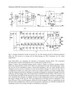
optimization process (see Fig. 4).
Once the nodes are deployed in the interested area, the network topology is first abstracted
and the overall network is partitioned into equivalent sub-networks that have the same
characteristics and where the energy consumption can be optimized independently but in
the same way. One mobile base station is then randomly deployed on the periphery of each
sub-network. Time is then divided into equal periods of time called rounds or epochs. At
the beginning of each round, each base station moves along the periphery of its
corresponding sub-network. Once it reached its new position, the base station collects
information about the current topology status of its sub-network. These information may
include The residual energy at each sensor node, the neighbors list and the positions of each
node, sources’ throughputs, etc.
In a next step, each base station runs the routing optimization process corresponding to its
sub-network as described in the previous section and which results in an updated routing
matrix that optimally distributes energy consumption over the different Cluster Heads
according to their roles in the sub-network and to the residual amount energy at each of
them. Data gathering is then performed by the sensing nodes and the collected data is
aggregated and forwarded by the cluster heads toward the corresponding base station using
the optimized routing probabilities.

Input: G(H, A).
0.1. The network is divided into N
b
equivalent sub-networks.
0.2. One mobile base station is deployed on the periphery of each of these sub-networks.
0.3. Initial round duration (epoch) is determined at the application level
While (the sensor network is operational for the application) do
{//begin of the round
k  {1
N
b
}:
1. Base station b
k
in sub-network k moves to its new position on the periphery
2. At base station b
k
: Collection of all relevant information from all the cluster heads of H
k

concerning the current topology of sub-network k.
3. At base station b
k
: Run of the optimization process and compute the routing matrix [P
k
].
4. Base station b
k
transmits to each Cluster Head CH
k,i

the vector [P
k,ij
]
(
i

{1 N
k
CH
} and

j /CH
k, j

L
k,i
).
5. Each Cluster Head sends the captured/received information to its neighbors toward b
k

according to [P
k
].

// end of the round}
Fig. 4. Global Framework.
Topology Control and Routing in Large Scale WSNs 243
Hence, according to the energy model described in section 4.2.3, the lifetime of CH
k,i
under a

given system
P
k
 p
k,ij




(k,i

{1 N
k
CH
})
is given by:
)12(
))((
)(
,
/ /
,,,,
,,
/ /
,,,,,,
,
,
/ /
,,,,
,

,,
,, ,,
,, ,,
,, ,,
2
jk
LCHj LCHj
jikrikijkijk
ikrajk
LCHj LCHj
jikrikijkijk
C
ik
CH
ik
C
ik
jk
LCHj LCHj
jikrikijkijk
CH
ik
C
ikk
CH
ik
wpewpe
reewpewpeTE
T
wpewpe

E
TPT
ikjk ikjk
ikjk ikjk
ikjk ikjk
 
 
 
 
 
 






Then,
T
k
, the lifetime of sub-graph k, can be approximated as follow:

)13(),(min)(
,
} 1{
kPTPT
k
CH
ik
Ni

kk
CH
k




Maximizing the lifetime of a sub-network k can be reached by solving the following
optimization problem:
} 1{
} 1{0
)14(/} 1{0
,,,
/
,
,,,
21
,,
CH
k
CH
ik
CH
ik
CH
ik
CH
k
LCHj
ijk

ikjk
CH
kijk
k
NiEEE
Nip
LCHjandNiptoSubject
TMaximize
ikjk






The last constraint models energy conservation at each Cluster Head CH
k,i
.
The resolution of this system requires determining the matrix P
k
defining, for a fixed
position of Base Station b
k
, the optimal routing flows that are used by each Cluster Head
within sub-network k to forward data to its Neighbors such that the lifetime of this sub-
network is maximized. The optimal matrix P
k
can then be computed in a centralized fashion
at the Base Station b
k

.
This optimisation problem is Non Polynomial and can then be solved over Matlab using
specific heuristics similar to those used to solve the optimization problem presented in
(Slama et al., 2006). Once the different sub-networks lifetimes

T
k
,

k 1to
N
b
are
computed, the whole network lifetime can be finally given by:

)15(min
k
k
net
TT



6. Global Framework
In this section we describe the overall dynamic framework for large two-tiered wireless
sensor networks lifetime maximization. The framework is based on the optimisation scheme
related to both Base Stations positioning and inter-Cluster Head communication presented
previously. A cyclic algorithm is then defined to permit the dynamic adaptation of the
optimization process (see Fig. 4).
Once the nodes are deployed in the interested area, the network topology is first abstracted

and the overall network is partitioned into equivalent sub-networks that have the same
characteristics and where the energy consumption can be optimized independently but in
the same way. One mobile base station is then randomly deployed on the periphery of each
sub-network. Time is then divided into equal periods of time called rounds or epochs. At
the beginning of each round, each base station moves along the periphery of its
corresponding sub-network. Once it reached its new position, the base station collects
information about the current topology status of its sub-network. These information may
include The residual energy at each sensor node, the neighbors list and the positions of each
node, sources’ throughputs, etc.
In a next step, each base station runs the routing optimization process corresponding to its
sub-network as described in the previous section and which results in an updated routing
matrix that optimally distributes energy consumption over the different Cluster Heads
according to their roles in the sub-network and to the residual amount energy at each of
them. Data gathering is then performed by the sensing nodes and the collected data is
aggregated and forwarded by the cluster heads toward the corresponding base station using
the optimized routing probabilities.

Input: G(H, A).
0.1. The network is divided into N
b
equivalent sub-networks.
0.2. One mobile base station is deployed on the periphery of each of these sub-networks.
0.3. Initial round duration (epoch) is determined at the application level
While (the sensor network is operational for the application) do
{//begin of the round
k  {1
N
b
}:
1. Base station b

k
in sub-network k moves to its new position on the periphery
2. At base station b
k
: Collection of all relevant information from all the cluster heads of H
k

concerning the current topology of sub-network k.
3. At base station b
k
: Run of the optimization process and compute the routing matrix [P
k
].
4. Base station b
k
transmits to each Cluster Head CH
k,i
the vector [P
k,ij
]
( i  {1 N
k
CH
} and j /CH
k, j
 L
k,i
).
5. Each Cluster Head sends the captured/received information to its neighbors toward b
k

according to [P
k
].

// end of the round}
Fig. 4. Global Framework.
Sustainable Wireless Sensor Networks244
7. Simulations
This section is dedicated to the evaluation of the performances of first, the Base Stations
Placement scheme that optimally locates the different base stations in the network while
considering scalability as well as energy efficiency issues and second, the inter-ClusterHead
communication approach formulated as an optimization problem that aims to efficiently
and fairly distribute the energy among Cluster Heads while taking into account their roles
in the network.

7.1 Base Stations placement
The effect of the proposed partitioning technique on the WSN lifetime is investigated using
numerical simulations over Matlab environment. A circular large-scale wireless sensor
network, with a radius R = 500m is considered. In order to study the performance of the
base stations placement scheme, we focused on the upper tier of the network architecture
(Base Stations and Cluster Heads) independently of the lower tier (Cluster Heads and
Sensing Nodes). 1000 nodes (Cluster Heads) are randomly (uniformly) deployed over a
network area. All nodes are similar with a communication range r = 80m and an initial
energy of 1000J unit. Base Stations are assumed to have no energy constraints because they
have larger batteries or their batteries are rechargeable. We assumed, in this scenario, that
the shortest path routing algorithm is used to establish routes from Cluster Heads to base
stations. The network lifetime is defined as the moment at which the first node runs out of
energy. Time is divided into rounds. Each round is composed of T =100 timeframes. Each
sensor node generates one data packet every timeframe.

To evaluate the efficiency of the proposed graph partitioning technique in elongating the
network lifetime, three comparative scenarios are considered:
1. Scenario 1:

Case 1: An entire large network (not partitioned) is considered. All the sensors have the
same capacity. N base stations are randomly fixed inside the coverage area of interest. Each
sensor has to send the data it senses to the nearest base station.
Case 2: The graph-partitioning algorithm (detailed in section 4.3.3) is used to define N
smaller sub-networks. One single base station is then randomly fixed in each sub network.
Each sensor node sends its data to the base station deployed inside the sub-network the
sensor node is belonging to.
2. Scenario 2:

Case 1: The entire network is considered. N mobile base stations are deployed randomly.
Then, the base stations start to move inside the area of interest following the random
waypoint model (Johnson & Maltz, 1996). At the beginning of each round, each base station
moves 60 m.
Case 2: N sub-networks are defined using the graph-partitioning algorithm and one single
base station is randomly deployed in each sub network. Then each base station moves 60m
each round. The base station cannot go outside the area of the sub-network it belongs to.
This area is represented by a disc with the geographic centre of the sub-network as centre
and the distance between this centre and the farthest sensor (belonging to this sub-network)
from it as radius.
3. Scenario 3:
Case 1: The entire network is considered. N mobile base stations are deployed randomly on
the periphery of the network. Then, the base stations start to move along the periphery. In
one round each base station moved 60 m.
Case 2: The graph-partitioning algorithm is used to define N smaller sub-networks. One
single base station is randomly deployed on the periphery of each sub network. Then each
base station moves 60m each round on the periphery.

We consider that the time required by a base station to move to its next position is negligible
compared to a round duration.
Several simulations are then run to compare the network lifetime in the two different cases
of each of the three different scenarios.
Simulation results are presented in fig. 5, 6 and 7. They respectively compare the
performance of the different base stations deployment strategies in the case of partitioned
and non-partitioned network (scenario 1, 2and 3).
First, let’s notice that the simple use of multiple base stations enhances the network lifetime
(with and without partitioning). Indeed, the network lifetime increases proportionally to the
number of base stations because the distance between the nodes and their correspondent
base stations is shortened. Second, it can be seen that moving the base stations clearly
prolong the operation of the network. In fact, figures show that the network lifetime is much
longer when the base stations are moving (scenario 2 and 3 with or without partitioning)
than when they are fix (scenario1). This result is valid with or without partitioning.
Third, enhancements of the network lifetime can be observed in the case of partitioned
large-scale WSNs compared to non-partitioned ones in all the scenarios. But the
enhancement is the most significant in the third scenario. This was expected as when one
base station is moving along the periphery of each sub-network, the energy consumption is
obviously much more distributed over the sensors than when all the base stations are
moving along the periphery of the whole network. The nodes that are the closest to the base
stations are logically the ones who die first because they not only send their own data but
also relay the data of all the nodes in the network. In scenario 3, the nodes who die first in
the case of non-partitioned network are the nodes situated all along the periphery whereas
in the case of partitioned network, they are the ones situated along the peripheries of the
different sub-networks. Then, in this scenario, using the graph partitioning technique to
deploy the base stations distributes the load relay and decreases the average distance
between the nodes and the base stations. Indeed, the improvement of the network lifetime
of the partitioned network is much more important when the number of base stations (or
sub-networks) increases.

Topology Control and Routing in Large Scale WSNs 245
7. Simulations
This section is dedicated to the evaluation of the performances of first, the Base Stations
Placement scheme that optimally locates the different base stations in the network while
considering scalability as well as energy efficiency issues and second, the inter-ClusterHead
communication approach formulated as an optimization problem that aims to efficiently
and fairly distribute the energy among Cluster Heads while taking into account their roles
in the network.

7.1 Base Stations placement
The effect of the proposed partitioning technique on the WSN lifetime is investigated using
numerical simulations over Matlab environment. A circular large-scale wireless sensor
network, with a radius R = 500m is considered. In order to study the performance of the
base stations placement scheme, we focused on the upper tier of the network architecture
(Base Stations and Cluster Heads) independently of the lower tier (Cluster Heads and
Sensing Nodes). 1000 nodes (Cluster Heads) are randomly (uniformly) deployed over a
network area. All nodes are similar with a communication range r = 80m and an initial
energy of 1000J unit. Base Stations are assumed to have no energy constraints because they
have larger batteries or their batteries are rechargeable. We assumed, in this scenario, that
the shortest path routing algorithm is used to establish routes from Cluster Heads to base
stations. The network lifetime is defined as the moment at which the first node runs out of
energy. Time is divided into rounds. Each round is composed of T =100 timeframes. Each
sensor node generates one data packet every timeframe.
To evaluate the efficiency of the proposed graph partitioning technique in elongating the
network lifetime, three comparative scenarios are considered:
1. Scenario 1:
Case 1: An entire large network (not partitioned) is considered. All the sensors have the
same capacity. N base stations are randomly fixed inside the coverage area of interest. Each
sensor has to send the data it senses to the nearest base station.
Case 2: The graph-partitioning algorithm (detailed in section 4.3.3) is used to define N

smaller sub-networks. One single base station is then randomly fixed in each sub network.
Each sensor node sends its data to the base station deployed inside the sub-network the
sensor node is belonging to.
2. Scenario 2:
Case 1: The entire network is considered. N mobile base stations are deployed randomly.
Then, the base stations start to move inside the area of interest following the random
waypoint model (Johnson & Maltz, 1996). At the beginning of each round, each base station
moves 60 m.
Case 2: N sub-networks are defined using the graph-partitioning algorithm and one single
base station is randomly deployed in each sub network. Then each base station moves 60m
each round. The base station cannot go outside the area of the sub-network it belongs to.
This area is represented by a disc with the geographic centre of the sub-network as centre
and the distance between this centre and the farthest sensor (belonging to this sub-network)
from it as radius.
3. Scenario 3:
Case 1: The entire network is considered. N mobile base stations are deployed randomly on
the periphery of the network. Then, the base stations start to move along the periphery. In
one round each base station moved 60 m.
Case 2: The graph-partitioning algorithm is used to define N smaller sub-networks. One
single base station is randomly deployed on the periphery of each sub network. Then each
base station moves 60m each round on the periphery.
We consider that the time required by a base station to move to its next position is negligible
compared to a round duration.
Several simulations are then run to compare the network lifetime in the two different cases
of each of the three different scenarios.
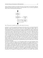
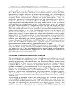
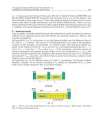
Simulation results are presented in fig. 5, 6 and 7. They respectively compare the
performance of the different base stations deployment strategies in the case of partitioned
and non-partitioned network (scenario 1, 2and 3).
First, let’s notice that the simple use of multiple base stations enhances the network lifetime
(with and without partitioning). Indeed, the network lifetime increases proportionally to the

number of base stations because the distance between the nodes and their correspondent
base stations is shortened. Second, it can be seen that moving the base stations clearly
prolong the operation of the network. In fact, figures show that the network lifetime is much
longer when the base stations are moving (scenario 2 and 3 with or without partitioning)
than when they are fix (scenario1). This result is valid with or without partitioning.
Third, enhancements of the network lifetime can be observed in the case of partitioned
large-scale WSNs compared to non-partitioned ones in all the scenarios. But the
enhancement is the most significant in the third scenario. This was expected as when one
base station is moving along the periphery of each sub-network, the energy consumption is
obviously much more distributed over the sensors than when all the base stations are
moving along the periphery of the whole network. The nodes that are the closest to the base
stations are logically the ones who die first because they not only send their own data but
also relay the data of all the nodes in the network. In scenario 3, the nodes who die first in
the case of non-partitioned network are the nodes situated all along the periphery whereas
in the case of partitioned network, they are the ones situated along the peripheries of the
different sub-networks. Then, in this scenario, using the graph partitioning technique to
deploy the base stations distributes the load relay and decreases the average distance
between the nodes and the base stations. Indeed, the improvement of the network lifetime
of the partitioned network is much more important when the number of base stations (or
sub-networks) increases.

Sustainable Wireless Sensor Networks246
0
50
100
150
200
250
300
350

400
450
2 4 8
number of sinks
lifetime duration (rounds)
case1
case2

Fig. 5. The network lifetime in the scenario 1.

0
100
200
300
400
500
600
700
800
900
1000
2 4 8
number of sinks
lifetime duration (rounds)
case1
case2

Fig. 6. The network lifetime in the scenario 2.

0

200
400
600
800
1000
1200
2 4 8
number of sinks
lifetime duration (rounds)
case1
case2

Fig. 7. The network lifetime in the scenario 3.

In the first case of the first scenario, base stations are randomly placed. Hence, they can be in
some cases grouped in a small space. As a consequence, the distance between a node and
the closest base station may not be really shortened. Whereas, in the second case, where we
limited the area in which each base station can be deployed, by partitioning the network
into sub networks, this distance is almost always shortened. This can be much more efficient
when the base stations move (scenario 2) since the base stations in both cases have the same
velocity (60m/round).
However, we notice, from fig. 5 and fig. 6, that the improvement is not so spectacular. This can
be explained by the fact that when dividing the network into independent sub-networks, some
nodes are bound to send their data to the base station deployed in the sub-network they
belong to whereas they are closer to a base station deployed outside (in an other sub-network).

7.2 Inter-Cluster Heads Communication
In this section, we focus on the performance evaluation of the optimization scheme presented
in section 4.4 and which manages the communication between Cluster Heads whithin each
sub-network to efficiently transmit data toward base stations. The optimization problem is

solved using specific heuristics and several simulations were run over Matlab.
Since the same optimal routing process is used in each of the sub-networks, we limit here
our simulations to one single sub-network. We consider then a circular sub-network with
radius equal to 100m. Cluster Heads and Sensing nodes are assumed to have a maximum
communication radius of 80m and 20m respectively. We assume that nodes are, initially,
distributed in a random fashion over the sub-area and that the clusterization is based on
neighborhood. Feasibles sets are then randomly generated in each cluster of the sub-
Topology Control and Routing in Large Scale WSNs 247
0
50
100
150
200
250
300
350
400
450
2 4 8
number of sinks
lifetime duration (rounds)
case1
case2

Fig. 5. The network lifetime in the scenario 1.

0
100
200
300

400
500
600
700
800
900
1000
2 4 8
number of sinks
lifetime duration (rounds)
case1
case2

Fig. 6. The network lifetime in the scenario 2.

0
200
400
600
800
1000
1200
2 4 8
number of sinks
lifetime duration (rounds)
case1
case2

Fig. 7. The network lifetime in the scenario 3.

In the first case of the first scenario, base stations are randomly placed. Hence, they can be in
some cases grouped in a small space. As a consequence, the distance between a node and
the closest base station may not be really shortened. Whereas, in the second case, where we
limited the area in which each base station can be deployed, by partitioning the network
into sub networks, this distance is almost always shortened. This can be much more efficient
when the base stations move (scenario 2) since the base stations in both cases have the same
velocity (60m/round).
However, we notice, from fig. 5 and fig. 6, that the improvement is not so spectacular. This can
be explained by the fact that when dividing the network into independent sub-networks, some
nodes are bound to send their data to the base station deployed in the sub-network they
belong to whereas they are closer to a base station deployed outside (in an other sub-network).

7.2 Inter-Cluster Heads Communication
In this section, we focus on the performance evaluation of the optimization scheme presented
in section 4.4 and which manages the communication between Cluster Heads whithin each
sub-network to efficiently transmit data toward base stations. The optimization problem is
solved using specific heuristics and several simulations were run over Matlab.
Since the same optimal routing process is used in each of the sub-networks, we limit here
our simulations to one single sub-network. We consider then a circular sub-network with
radius equal to 100m. Cluster Heads and Sensing nodes are assumed to have a maximum
communication radius of 80m and 20m respectively. We assume that nodes are, initially,
distributed in a random fashion over the sub-area and that the clusterization is based on
neighborhood. Feasibles sets are then randomly generated in each cluster of the sub-
Sustainable Wireless Sensor Networks248
network. One base station with no energy constraints is deployed and randomly placed on
the periphery of the area.
The same initial energy is assumed for all Cluster Heads and is equal to 1000 J unit. The
same initial energy is also assumed for all Sensing Nodes and is equal to 50 J. Power
consumption at the Sensing Nodes is 10 µW.
The following values are considered for energy dissipation at Cluster Heads.

E
elec
=50nJ/bit in the transmit circuitry and
є
amp
=100pJ/bit/m
2
for the transmit amplifier.

= 50nJ/bit for the aggregation energy consumption.
We assume the data aggregation ratio

=25% and a Sensing Node data rate equal to 160bit/s.
Figures are obtained by averaging simulation results for a large number of scenarios. For
each scenario, a different random node layout is used.
Fig. 8 illustrates the normalized sub-network lifetime. As depicted, the numerical resolution
of the proposed model quickly converges to an optimal solution.
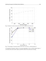
To study the effect of the sub-network composition and topology on its lifetime and the
interactions between the inter-cluster and intra-cluster communications, we study the
scenario where the size of the clusters vary while the number of cluster heads is kept
constant. When running the simulations, we randomly generate feasible sets for each
cluster. The number of feasible sets in a cluster is randomly chosen. The number of cluster
heads is fixed at 20. Initially, we randomly generate the number of sensing nodes in each
cluster while keeping the average number equal to 3. Then, we increase the number of
sensing nodes similarly in each cluster until it reaches 18 (average size).
The results are presented in fig. 9, which illustrates a sub-network lifetime evolution when
increasing the clusters’ size and keeping the number of cluster heads constant.
It can be seen that the sub-network lifetime decreases as the clusters size increases. This is
expected as when the cluster size increases, the corresponding cluster lifetime increases as
well. Hence, each cluster head will spend more time performing both its neighbor’s data

relay and its own cluster management (its two roles simultaneously). As a result, it expends
more quickly its energy which leads to network death in shorter time.
To further explore the performances of the proposed inter-cluster head communication
scheme, we propose to study the influence of the clusters lifetime on the choice of the routes
to deliver the data from each Cluster Head to the base station. An efficient routing scheme
should alleviate from releying tasks cluster heads with long clusters lifetime since these
cluster heads will spend longer time and then much more energy to manage their clusters
than those with short cluster lifetime. To this end, we voluntarily generate clusters with
considerably different lifetimes (through different sizes). This makes the corresponding
clusters’ lifetime standard deviation be large.
After several simulations, we compute the different cluster head lifetime and we remark
that the corresponding standard deviation is considerably small (3.2% of the whole sub-
network lifetime). This result proves that the majority of cluster heads die approximately at
the same time. This also proves that flows are fairly distributed over the different cluster
heads proportionally to the residual energy available at each one of them and also with
considering the lifetime of each cluster i.e., proportionally to their role in the sub-network.
The objectives of the proposed schemes are obviously attained.

Fig. 8. Lifetime convergence.


Fig. 9. Sub-network lifetime as a function of the clusters size.
Topology Control and Routing in Large Scale WSNs 249
network. One base station with no energy constraints is deployed and randomly placed on
the periphery of the area.
The same initial energy is assumed for all Cluster Heads and is equal to 1000 J unit. The
same initial energy is also assumed for all Sensing Nodes and is equal to 50 J. Power
consumption at the Sensing Nodes is 10 µW.
The following values are considered for energy dissipation at Cluster Heads.
E

elec
=50nJ/bit in the transmit circuitry and
є
amp
=100pJ/bit/m
2
for the transmit amplifier.

= 50nJ/bit for the aggregation energy consumption.
We assume the data aggregation ratio

=25% and a Sensing Node data rate equal to 160bit/s.
Figures are obtained by averaging simulation results for a large number of scenarios. For
each scenario, a different random node layout is used.
Fig. 8 illustrates the normalized sub-network lifetime. As depicted, the numerical resolution
of the proposed model quickly converges to an optimal solution.
To study the effect of the sub-network composition and topology on its lifetime and the
interactions between the inter-cluster and intra-cluster communications, we study the
scenario where the size of the clusters vary while the number of cluster heads is kept
constant. When running the simulations, we randomly generate feasible sets for each
cluster. The number of feasible sets in a cluster is randomly chosen. The number of cluster
heads is fixed at 20. Initially, we randomly generate the number of sensing nodes in each
cluster while keeping the average number equal to 3. Then, we increase the number of
sensing nodes similarly in each cluster until it reaches 18 (average size).
The results are presented in fig. 9, which illustrates a sub-network lifetime evolution when
increasing the clusters’ size and keeping the number of cluster heads constant.
It can be seen that the sub-network lifetime decreases as the clusters size increases. This is
expected as when the cluster size increases, the corresponding cluster lifetime increases as
well. Hence, each cluster head will spend more time performing both its neighbor’s data
relay and its own cluster management (its two roles simultaneously). As a result, it expends

more quickly its energy which leads to network death in shorter time.
To further explore the performances of the proposed inter-cluster head communication
scheme, we propose to study the influence of the clusters lifetime on the choice of the routes
to deliver the data from each Cluster Head to the base station. An efficient routing scheme
should alleviate from releying tasks cluster heads with long clusters lifetime since these
cluster heads will spend longer time and then much more energy to manage their clusters
than those with short cluster lifetime. To this end, we voluntarily generate clusters with
considerably different lifetimes (through different sizes). This makes the corresponding
clusters’ lifetime standard deviation be large.
After several simulations, we compute the different cluster head lifetime and we remark
that the corresponding standard deviation is considerably small (3.2% of the whole sub-
network lifetime). This result proves that the majority of cluster heads die approximately at
the same time. This also proves that flows are fairly distributed over the different cluster
heads proportionally to the residual energy available at each one of them and also with
considering the lifetime of each cluster i.e., proportionally to their role in the sub-network.
The objectives of the proposed schemes are obviously attained.

Fig. 8. Lifetime convergence.


Fig. 9. Sub-network lifetime as a function of the clusters size.
Sustainable Wireless Sensor Networks250
8. Conclusion
The use of multiple mobile base stations in large-scale wireless sensor networks is necessary
in order to cover large areas and to minimize energy consumption for data transmission
operations. In this chapter, we proposed an energy efficient usage of multiple, mobile base
stations to increase the lifetime of a two-tiered large-scale Wireless Sensor Network. Our
approach uses a graph-partitioning algorithm to decompose the underlying network into
balanced sub-networks. The energy usage is then optimized in each sub-network
independently but in the same way using efficient base stations placement techniques that

are optimized for small-scale WSNs. Performance results have shown that the proposed
technique considerably enhances the network lifetime particularly when the base stations
are moving along the periphery.
We have further proposed an optimal multi-hop routing scheme used within each sub-
network independently to efficiently manage the communication between the Cluster
Heads so that the entire network lifetime is elongated. Different strategies can be used,
inside clusters, to manage intra-cluster communications. The proposed scheme simply adapt
and fairly distribute the relaying flows according to Cluster Heads residual energy and their
corresponding Clusters’ lifetime duration, so that Cluster Heads with critical energy
situations are alleviated from relaying operations. Simulation results have shown that we
can compute a near optimal solution of the routing matrix that defines the optimal flow
routing.
The overall dynamic framework that combines the above two schemes has been then
described. It is defined as a cyclic algorithm that allows dynamic adaptation of the
optimization process according to the current status of the whole network.
Using the graph-partitioning approach to improve energy consumption in large-scale WSNs
is promising. We will focus in complementary and future work on more elaborated
approaches for optimal multiple mobile base stations placement and WSN partitioning. In
addition, efficient tools should be proposed to determine the optimal number of partitions
and base stations to be used according to the WSN characteristics, applications’
requirements and financial costs.
Moreover, we plan in future work to investigate further the mathematical resolution of the
optimization algorithm corresponding to the inter-Cluster Head communication. The effect
on energy consumption of the overhead generated by this scheme needs to be more deeply
explored.

9. References
Chatterjee, M.; Das, S.K. & Turgut, D. (2002). WCA: A Weighted Clustering Algorithm for
Mobile Ad hoc Networks, Journal of Cluster Computing, special issue on Mobile Ad hoc
Networking, vol. 5, (march 2002), (pp.193-204).

Chen, Y. P.; Liestman, A. L. & Liu, J. (2006). A Hierarchical Energy-Efficient Framework for
Data Aggregation in Wireless Sensor Networks, IEEE Transactions on Vehicular
Technology, vol. 55, no. 3 , (May 2006) (789-796).
Chen, C.; Ma, J. & Yu, K. (2006). Designing Energy-Efficient Wireless Sensor Networks with
Mobile Sinks, Proceeding of ACM Sensys Workshop WSW, pp. 1-9, USA, Colorado,
October 2006, Boulder.
Chlebikova, J. (1996). Approximability of the Maximally balanced connected partition
problem in graphs, Information Processing Letters, vol. 60, (sept 1996), (pp.225 – 230).
Even, G.; Naor, J.; Rao, S. & Schieber, B. (1997). Fast approximate graph partitioning
algorithms, Proceeding of the 8th Annual ACM-SIAM Symposium on Discrete
Algorithms, pp. 639-648, USA, LA, 1997, New Orleans.
Gandham, S.R.; Dawande, M. ; Prakash, R. & Venkatesan, S. (2003). Energy Efficient
Schemes for Wireless Sensor Networks With Multiple Mobile Base Stations,
Proceeding of IEEE GLOBECOM, pp. 377-381, USA, California, may 2003, San
Francisco.
Ito, T.; Zhou, X. & Nishizeki, T. (2006). Partitioning a graph of bounded tree-width to
connected subgraphs of almost uniform size, Journal of discrete algorithms, Vo. 4, Iss.
1, (March 2006), (pp. 142-154).
Johnson, D. B. & Maltz, D. A. (1996). Dynamic source routing in ad hoc wireless networks,
Mobile Computing, Vol. 353, (August 1996), (pp. 153-181).
Kim, H.; Seok, Y.; Choi, N.; Choi, Y. & Kwon, T. (2006). “Optimal Multi-sink Positioning
and Energy-efficient Routing in Wireless Sensor Networks, Lecture Notes in
Computer Science, Vol.3391, Note(s):XVII, 936,Document:11, (sept 2006), (pp.264-
274).
Luo, J.; Panchard, J.; Piorkowski, M.; Grosglausser, M. & Hubaux, J-P. (2006). Mobiroute:
Routing towards a Mobile Sink for Improving Lifetime in Sensor Networks,
Proceeding of the International Conference on Distributed Computing in Sensor Systems,
pp. 480-497, USA, California, June 2006, San Francisco.
Luo, J. & Hubaux, J P. (2005). Joint Mobility and Routing for Lifetime Elongation in
Wireless Sensor Networks, Proceeding of IEEE INFOCOM, pp. 1-10, USA, March

2005, Miami.
Mhatre, V.; Rosenberg, C.; Kofman, D.; Mazumdar, R. & Shroff, N. (2005). A Minimum Cost
Heterogeneous Sensor Network with a Lifetime Constraint, IEEE Transaction on
Mobile Computing, vol. 4, no. 1, (sept 2005), (pp 4-15).
Pan, J.; Hou, Y.; Cai, L.; Shi, Y. & Shen, X. (2003). Topology control for wireless sensor
networks, Proceeding of the 9th ACM Conference on Mobile Computing and Networking,
pp. 286-299, USA, CA, September 2003, San Diego.
Perillo, M. & Heinzelman, W. (2003). Optimal Sensor Management Under Energy and
Reliability Constraints, Proceedings of the IEEE Wireless Communications and
Networking Conference, pp.1-6, USA, Louisiana, March 2003, New Orleans.
Rabiner Heinzelman, W.; Chandrakasan, A. & Balakrishnan, H. (2000). Energy-Efficient
Communication Protocol for Wireless Microsensor Networks, Proceedings of the 33rd
International Conference on System Sciences, pp. 3005-3014, USA, January 2000,
Hawaii.
Rabiner Heinzelman, W.; Chandrakasan, A. & Balakrishnan, H (2002). An Application-
Specific Protocol Architecture for Wireless Microsensor Networks, IEEE Transaction
in Wireless Communications, vol. 1, no. 4, (Oct. 2002), (pp. 660-670).
Topology Control and Routing in Large Scale WSNs 251
8. Conclusion
The use of multiple mobile base stations in large-scale wireless sensor networks is necessary
in order to cover large areas and to minimize energy consumption for data transmission
operations. In this chapter, we proposed an energy efficient usage of multiple, mobile base
stations to increase the lifetime of a two-tiered large-scale Wireless Sensor Network. Our
approach uses a graph-partitioning algorithm to decompose the underlying network into
balanced sub-networks. The energy usage is then optimized in each sub-network
independently but in the same way using efficient base stations placement techniques that
are optimized for small-scale WSNs. Performance results have shown that the proposed
technique considerably enhances the network lifetime particularly when the base stations
are moving along the periphery.
We have further proposed an optimal multi-hop routing scheme used within each sub-

network independently to efficiently manage the communication between the Cluster
Heads so that the entire network lifetime is elongated. Different strategies can be used,
inside clusters, to manage intra-cluster communications. The proposed scheme simply adapt
and fairly distribute the relaying flows according to Cluster Heads residual energy and their
corresponding Clusters’ lifetime duration, so that Cluster Heads with critical energy
situations are alleviated from relaying operations. Simulation results have shown that we
can compute a near optimal solution of the routing matrix that defines the optimal flow
routing.
The overall dynamic framework that combines the above two schemes has been then
described. It is defined as a cyclic algorithm that allows dynamic adaptation of the
optimization process according to the current status of the whole network.
Using the graph-partitioning approach to improve energy consumption in large-scale WSNs
is promising. We will focus in complementary and future work on more elaborated
approaches for optimal multiple mobile base stations placement and WSN partitioning. In
addition, efficient tools should be proposed to determine the optimal number of partitions
and base stations to be used according to the WSN characteristics, applications’
requirements and financial costs.
Moreover, we plan in future work to investigate further the mathematical resolution of the
optimization algorithm corresponding to the inter-Cluster Head communication. The effect
on energy consumption of the overhead generated by this scheme needs to be more deeply
explored.

9. References
Chatterjee, M.; Das, S.K. & Turgut, D. (2002). WCA: A Weighted Clustering Algorithm for
Mobile Ad hoc Networks, Journal of Cluster Computing, special issue on Mobile Ad hoc
Networking, vol. 5, (march 2002), (pp.193-204).
Chen, Y. P.; Liestman, A. L. & Liu, J. (2006). A Hierarchical Energy-Efficient Framework for
Data Aggregation in Wireless Sensor Networks, IEEE Transactions on Vehicular
Technology, vol. 55, no. 3 , (May 2006) (789-796).
Chen, C.; Ma, J. & Yu, K. (2006). Designing Energy-Efficient Wireless Sensor Networks with

Mobile Sinks, Proceeding of ACM Sensys Workshop WSW, pp. 1-9, USA, Colorado,
October 2006, Boulder.
Chlebikova, J. (1996). Approximability of the Maximally balanced connected partition
problem in graphs, Information Processing Letters, vol. 60, (sept 1996), (pp.225 – 230).
Even, G.; Naor, J.; Rao, S. & Schieber, B. (1997). Fast approximate graph partitioning
algorithms, Proceeding of the 8th Annual ACM-SIAM Symposium on Discrete
Algorithms, pp. 639-648, USA, LA, 1997, New Orleans.
Gandham, S.R.; Dawande, M. ; Prakash, R. & Venkatesan, S. (2003). Energy Efficient
Schemes for Wireless Sensor Networks With Multiple Mobile Base Stations,
Proceeding of IEEE GLOBECOM, pp. 377-381, USA, California, may 2003, San
Francisco.
Ito, T.; Zhou, X. & Nishizeki, T. (2006). Partitioning a graph of bounded tree-width to
connected subgraphs of almost uniform size, Journal of discrete algorithms, Vo. 4, Iss.
1, (March 2006), (pp. 142-154).
Johnson, D. B. & Maltz, D. A. (1996). Dynamic source routing in ad hoc wireless networks,
Mobile Computing, Vol. 353, (August 1996), (pp. 153-181).
Kim, H.; Seok, Y.; Choi, N.; Choi, Y. & Kwon, T. (2006). “Optimal Multi-sink Positioning
and Energy-efficient Routing in Wireless Sensor Networks, Lecture Notes in
Computer Science, Vol.3391, Note(s):XVII, 936,Document:11, (sept 2006), (pp.264-
274).
Luo, J.; Panchard, J.; Piorkowski, M.; Grosglausser, M. & Hubaux, J-P. (2006). Mobiroute:
Routing towards a Mobile Sink for Improving Lifetime in Sensor Networks,
Proceeding of the International Conference on Distributed Computing in Sensor Systems,
pp. 480-497, USA, California, June 2006, San Francisco.
Luo, J. & Hubaux, J P. (2005). Joint Mobility and Routing for Lifetime Elongation in
Wireless Sensor Networks, Proceeding of IEEE INFOCOM, pp. 1-10, USA, March
2005, Miami.
Mhatre, V.; Rosenberg, C.; Kofman, D.; Mazumdar, R. & Shroff, N. (2005). A Minimum Cost
Heterogeneous Sensor Network with a Lifetime Constraint, IEEE Transaction on
Mobile Computing, vol. 4, no. 1, (sept 2005), (pp 4-15).

Pan, J.; Hou, Y.; Cai, L.; Shi, Y. & Shen, X. (2003). Topology control for wireless sensor
networks, Proceeding of the 9th ACM Conference on Mobile Computing and Networking,
pp. 286-299, USA, CA, September 2003, San Diego.
Perillo, M. & Heinzelman, W. (2003). Optimal Sensor Management Under Energy and
Reliability Constraints, Proceedings of the IEEE Wireless Communications and
Networking Conference, pp.1-6, USA, Louisiana, March 2003, New Orleans.
Rabiner Heinzelman, W.; Chandrakasan, A. & Balakrishnan, H. (2000). Energy-Efficient
Communication Protocol for Wireless Microsensor Networks, Proceedings of the 33rd
International Conference on System Sciences, pp. 3005-3014, USA, January 2000,
Hawaii.
Rabiner Heinzelman, W.; Chandrakasan, A. & Balakrishnan, H (2002). An Application-
Specific Protocol Architecture for Wireless Microsensor Networks, IEEE Transaction
in Wireless Communications, vol. 1, no. 4, (Oct. 2002), (pp. 660-670).
Sustainable Wireless Sensor Networks252
Slama, I.; Jouaber, B. & Zeghlache, D. (2006). Routing for wireless sensor networks lifetime
maximization under energy constraints, Preceeding of the 3rd International Conference
on Mobile Technology, Applications and Systems, pp.1-5, Thailand, October 2006,
Bangkok.
Vincze, Z. ; Fodor, K. ; Vida, R. & Vidacs, A. (2006). Electrostatic Modelling of Multiple
Mobile Sinks in Wireless Sensor Networks, Proceeding of IFIP Networking Workshop
on Performance Control in Wireless Sensor Networks, pp. 30-37, Portugal, May 2006,
Coimbra.
Wang, Z. M.; Basagni, S.; Melachrinoudis, E. & Petrioli, C. (2005). Exploiting Sink Mobility
for Maximizing Sensor Networks Lifetime, Proceedings of the 38th Annual Hawaii
International Conference on System Sciences, pp. 287.1, USA, January 2005,
Washington, DC.

Dynamic Routing Framework for Wireless Sensor Networks 253
Dynamic Routing Framework for Wireless Sensor Networks
Mukundan Venkataraman, Mainak Chatterjee and Kevin Kwiat

1
Dynamic Routing Framework
for Wireless Sensor Networks
∗
Mukundan Venkataraman and Mainak Chatterjee
University of Central Florida
U.S.A.
Kevin Kwiat
Air Force Research Laboratory
U.S.A.
Abstract
Numerous routing protocols have been proposed for wireless sensor networks. Each such
protocol carries with it a set of assumptions about the traffic type that it caters to, and hence
has limited interoperability. Also, most protocols are validated over workloads which only
form a fraction of an actual deployment’s requirement. Most real world and commercial de-
ployments, however, would generate multiple traffic types simultaneously throughout the
lifetime of the network. For example, most deployments would want all of the following
to happen concurrently from the network: periodic reliable sense and disseminate, real time
streams, patched updates, network reprogramming, query-response dialogs, mission critical
alerts and so on. Naturally, no one routing protocol can completely cater to all of a deploy-
ments requirements.
This chapter presents a routing framework that captures the communication intent of an ap-
plication by using just three bits. The traditional routing layer is replaced with a collection
of routing components that can cater to various communication patterns. The framework dy-
namically switches routing component for every packet in question. Data structure require-
ments of component protocols are regularized, and core protocol features are distilled to build
a highly composable collection of routing modules. This creates a framework for developing,
testing, integrating, and validating protocols that are highly portable from one deployment
to another. Communication patterns can be easily described to lower layer protocols using
this framework. One such real world application scenario is also investigated: that of predic-

tive maintenance (PdM). The requirements of a large scale PdM are used to generate a fairly
complete and realistic traffic workload to drive an evaluation of such a framework.
1. Introduction
First generation wireless sensor networks (hereafter ‘sensornets’) passively transported bits
from one end to another. The subjective requirements of a payload are opaque to the network
∗
Approved for Public Release; Distribution Unlimited: 88ABW-2010-5582 dated 18 October 2010.
11
Sustainable Wireless Sensor Networks254
protocols, and the role of in-network processing is limited. Various routing protocols for trans-
porting data in sensornets have been proposed: protocols for reliable routing (2; 7; 24; 27; 28),
real time communication (10; 11; 14), energy aware communication (1; 12; 29), load balanced
communication, aggregation centric approaches (19) and so on to name a few. Each such pro-
tocol typically optimizes a certain set of chosen parameters in making routing decisions, and
is likewise validated over a workload that only generates that type of network traffic. This
means that a deployment that adopts any given protocol has to build its entire deployment
logic using the traffic type for which the protocol is optimized. To make sensornets a viable
solution to real world problems, applications need to be built on top of arbitrary communica-
tion patterns, often with conflicting requirements. For example, a meaningful case of habitat
monitoring would mostly demand all of the following communication patterns to co-exist:
periodic network reports using reliable sense and disseminate, critical real time alerts when
anomaly is detected, aggregation to suppress duplicates, network reprogramming to transfer
bulk data, patched updates for continuous customization of the sensornet, best effort com-
munication to transfer redundant information, interactivity with the network in the form of
request-reply dialogs and so on. Naturally, no one routing protocol can cater to such varied
application requirements within a given deployment. In other words, a given deployment can
be viewed as a collection of various tasks (applications) which have very different, and often
conflicting, communication requirements. The deployment goal is met when the goals of its
constituent applications are fulfilled.
Secondly, there is little synergy across research efforts. Pressed by scarcity of energy and a

need to focus on performance, protocols are developed with little thoughts to modularity and
interoperability. Though a new application deployment would have a plethora of routing
protocols to choose from, these protocols cannot be readily wired together to form a com-
municating framework due to compatibility problems. Compatibility problems largely arise
because of the assumptions made on interface and data structure requirements. In general,
and as Culler et. at. (5) note, a framework for testing, integrating and proposing protocols is
largely missing.
This chapter presents a routing framework that makes an application’s communication re-
quirements visible to the lower layers, and allows activation of application specific process-
ing. The traditional routing layer is replaced by a highly composable collection of routing
decisions. Now, the routing logic is dynamically wired as per each packets requirements.
The effectiveness of this strategy is demonstrated by gathering requirements and validating a
fairly complete deployment scenario: predictive maintenance (PdM) using sensornets (15).
2. Protocol Description
2.1 Routing Framework Overview
Application payload presents a three bit preamble to the framework that describes it commu-
nication intent, The framework dynamically switches routing decisions based on the preamble
bits. The routing layer is now a composable set of routing components that perform similar
functions, but are optimized for different classes of traffic. The routing components carry a
similar three bit signature that lets the framework know their applicability for a certain class
of traffic. The selection of a routing component is hence a mapping between what the appli-
cation demands and what the component has to offer. The routing components house core
protocol features that cater to a particular application type. This allows components to evolve
independently, and owing to their composable nature, allows seamless migration from one
deployment experience to another. To unify interface assumptions, the routing components
share a universal neighbor lookup table that houses relevant information about various neigh-
bors which saves storage space and makes way for consistent interface assumptions. Compo-
nent protocols make ranged queries into the neighbor table to derive the best candidate hop
for a given application payload. Designing such a framework requires addressing challenges
of composing routing protocols into core components, and regularizing the various interface

and data structure requirements. But before that, we begin with the fundamental problem of
making visible an applications demands to the stack.
2.2 Specifying Communication Intent
Applications need a way to express their communication requirements in a format that is both
completely expressive and minimal. Various approaches have been taken to increase applica-
tion visibility to the communication framework, and much of the effort has been to prioritize
data. For example, the SP architecture (20) argues for a one bit descriptor that describes the
urgency of a packet. On the Internet, DiffServ uses a class of service (CoS) field, three bits in
length, to specify a priority value between 0 (for best effort traffic) to 7 (real time traffic). ISP’s
in the present day Internet also use similar tags to differentially route packets from preferred
customers and offer them a higher quality of service. However, assigning a priority for any
class of traffic is a highly subjective task, and these assignment rules would not be consistent
from one deployment to another. Application naming should instead revolve around funda-
mental communication requirements rather than blatant priorities. This would allow one to
construct meaningful and consistent inferences of a packets requirement for virtually any de-
ployment. In effect, the following question is posed: What is the minimum number of bits to let a
deployment specify its fundamental communication requirements?
To best characterize an application to the communication framework, various possibilities
exist: number of recipients (anycast, multicast, broadcast), loss tolerance, delay tolerance,
priority, sensitivity to congestion or link losses, soliciting retransmissions, tagging packets for
aggregation, tagging packets for load balancing, control information v/s data packets and so
on. However, communication patterns can be best described using three fundamental axes:
nature of payload, reliability, and time criticality.
Nature of payload: Traffic in the network can be broadly classified as data or control traf-
fic. Data traffic is all of the push based traffic generated by a mote. Control traffic is traffic
used for control plane management (like beacons, ACK’s etc.), and to a certain extent, user
generated traffic. Sensor networks are more than just a collection of data gathering elements
that autonomously report values. There is a need to accommodate a human element into the
network for a variety of reasons. Users would want interact with the network with queries,
and would want to receive responses in short turn around times. More importantly, admin-

istrators see the need to continuously customize the network with updates or network repro-
gramming. Interplay of data and control traffic in the network needs to be closely modeled as
per a deployments requirements.
Reliability: The second axis to consider is tolerance to loss. Since a deployment consists
of a host of nodes that are primarily involved in data gathering, some level of redundancy
is sensed values is inherent. However, dictated by application requirements, some sensed
values might be loss intolerant. For example, a deployment might want to construct a time
series plot of sensed values from every mote for statistical purposes. This would require
every mote to reliably transfer data periodically with minimum losses. Loss intolerance is
also required for network re-programming or bulk reliable transfers, where binary updates
need to be transmitted to node(s) reliably over the network.
Dynamic Routing Framework for Wireless Sensor Networks 255
protocols, and the role of in-network processing is limited. Various routing protocols for trans-
porting data in sensornets have been proposed: protocols for reliable routing (2; 7; 24; 27; 28),
real time communication (10; 11; 14), energy aware communication (1; 12; 29), load balanced
communication, aggregation centric approaches (19) and so on to name a few. Each such pro-
tocol typically optimizes a certain set of chosen parameters in making routing decisions, and
is likewise validated over a workload that only generates that type of network traffic. This
means that a deployment that adopts any given protocol has to build its entire deployment
logic using the traffic type for which the protocol is optimized. To make sensornets a viable
solution to real world problems, applications need to be built on top of arbitrary communica-
tion patterns, often with conflicting requirements. For example, a meaningful case of habitat
monitoring would mostly demand all of the following communication patterns to co-exist:
periodic network reports using reliable sense and disseminate, critical real time alerts when
anomaly is detected, aggregation to suppress duplicates, network reprogramming to transfer
bulk data, patched updates for continuous customization of the sensornet, best effort com-
munication to transfer redundant information, interactivity with the network in the form of
request-reply dialogs and so on. Naturally, no one routing protocol can cater to such varied
application requirements within a given deployment. In other words, a given deployment can
be viewed as a collection of various tasks (applications) which have very different, and often

conflicting, communication requirements. The deployment goal is met when the goals of its
constituent applications are fulfilled.
Secondly, there is little synergy across research efforts. Pressed by scarcity of energy and a
need to focus on performance, protocols are developed with little thoughts to modularity and
interoperability. Though a new application deployment would have a plethora of routing
protocols to choose from, these protocols cannot be readily wired together to form a com-
municating framework due to compatibility problems. Compatibility problems largely arise
because of the assumptions made on interface and data structure requirements. In general,
and as Culler et. at. (5) note, a framework for testing, integrating and proposing protocols is
largely missing.
This chapter presents a routing framework that makes an application’s communication re-
quirements visible to the lower layers, and allows activation of application specific process-
ing. The traditional routing layer is replaced by a highly composable collection of routing
decisions. Now, the routing logic is dynamically wired as per each packets requirements.
The effectiveness of this strategy is demonstrated by gathering requirements and validating a
fairly complete deployment scenario: predictive maintenance (PdM) using sensornets (15).
2. Protocol Description
2.1 Routing Framework Overview
Application payload presents a three bit preamble to the framework that describes it commu-
nication intent, The framework dynamically switches routing decisions based on the preamble
bits. The routing layer is now a composable set of routing components that perform similar
functions, but are optimized for different classes of traffic. The routing components carry a
similar three bit signature that lets the framework know their applicability for a certain class
of traffic. The selection of a routing component is hence a mapping between what the appli-
cation demands and what the component has to offer. The routing components house core
protocol features that cater to a particular application type. This allows components to evolve
independently, and owing to their composable nature, allows seamless migration from one
deployment experience to another. To unify interface assumptions, the routing components
share a universal neighbor lookup table that houses relevant information about various neigh-
bors which saves storage space and makes way for consistent interface assumptions. Compo-

nent protocols make ranged queries into the neighbor table to derive the best candidate hop
for a given application payload. Designing such a framework requires addressing challenges
of composing routing protocols into core components, and regularizing the various interface
and data structure requirements. But before that, we begin with the fundamental problem of
making visible an applications demands to the stack.
2.2 Specifying Communication Intent
Applications need a way to express their communication requirements in a format that is both
completely expressive and minimal. Various approaches have been taken to increase applica-
tion visibility to the communication framework, and much of the effort has been to prioritize
data. For example, the SP architecture (20) argues for a one bit descriptor that describes the
urgency of a packet. On the Internet, DiffServ uses a class of service (CoS) field, three bits in
length, to specify a priority value between 0 (for best effort traffic) to 7 (real time traffic). ISP’s
in the present day Internet also use similar tags to differentially route packets from preferred
customers and offer them a higher quality of service. However, assigning a priority for any
class of traffic is a highly subjective task, and these assignment rules would not be consistent
from one deployment to another. Application naming should instead revolve around funda-
mental communication requirements rather than blatant priorities. This would allow one to
construct meaningful and consistent inferences of a packets requirement for virtually any de-
ployment. In effect, the following question is posed: What is the minimum number of bits to let a
deployment specify its fundamental communication requirements?
To best characterize an application to the communication framework, various possibilities
exist: number of recipients (anycast, multicast, broadcast), loss tolerance, delay tolerance,
priority, sensitivity to congestion or link losses, soliciting retransmissions, tagging packets for
aggregation, tagging packets for load balancing, control information v/s data packets and so
on. However, communication patterns can be best described using three fundamental axes:
nature of payload, reliability, and time criticality.
Nature of payload: Traffic in the network can be broadly classified as data or control traf-
fic. Data traffic is all of the push based traffic generated by a mote. Control traffic is traffic
used for control plane management (like beacons, ACK’s etc.), and to a certain extent, user
generated traffic. Sensor networks are more than just a collection of data gathering elements

that autonomously report values. There is a need to accommodate a human element into the
network for a variety of reasons. Users would want interact with the network with queries,
and would want to receive responses in short turn around times. More importantly, admin-
istrators see the need to continuously customize the network with updates or network repro-
gramming. Interplay of data and control traffic in the network needs to be closely modeled as
per a deployments requirements.
Reliability: The second axis to consider is tolerance to loss. Since a deployment consists
of a host of nodes that are primarily involved in data gathering, some level of redundancy
is sensed values is inherent. However, dictated by application requirements, some sensed
values might be loss intolerant. For example, a deployment might want to construct a time
series plot of sensed values from every mote for statistical purposes. This would require
every mote to reliably transfer data periodically with minimum losses. Loss intolerance is
also required for network re-programming or bulk reliable transfers, where binary updates
need to be transmitted to node(s) reliably over the network.
Sustainable Wireless Sensor Networks256
Application Payload
Control / Data
Delay Sensitivity
Reliability
Fig. 1. 3-bit preamble appended to the application payload
Time Criticality: Some sensed value might be of no use if it does not make it to the destination
within strict time bounds. Consider a deployment of sensors that report real time co-ordinates
of moving objects to a camera which then pans and zooms to that area. If the co-ordinates
reach the destination late, the camera might be unable to capture the desired frames of interest.
Again, dictated by application requirements, there are time bounds for values of interest to
make it to the destination.
2.3 Preamble Bits
Figure 1 shows the three axes of communications reduced to a simple three bit scheme that
each packet carries. These bits are set or unset by the application programmer using simple
API calls. The three bits, taken in combination, provide a characteristic description of an ap-

plications requirements. Figure 2 provides a complete combination of the preamble bits and
their inference. For example, a beacon packet would carry a signature of [1,0,0], denoting a
control packet that is loss tolerant and insensitive to delay. A data packet demanding reliabil-
ity over delay would publish [0,0,1]. Similarly, a real time packet which only demands speed
of delivery would publish [0,1,0]. An anomalous case is made when a packet demands both
reliability and speed of delivery (bits [0,1,1] and [1,1,1]). Ensuring reliability inherently adds
delay in transit, and such packets are interpreted as “mission critical", which see the need to
both make it to the destination and in as short a time as possible. In general, the bits when
combined with other information available in the packet headers make way for a powerful
expression of precise communication demands. Note that the bits do not convey any notion
of relative priority amongst packets, just a set of actual communication requirements.
2.4 Shared Neighbor Table: Unified view for routing protocols
Since the routing layer is now a collection of independent routing components, each com-
ponent assumes the presence of various state information to be available to perform routing
decisions. The neighbor table houses values such as the node-ID, energy available, congestion
level, depth, link-quality estimate and a ‘last heard’ bit. The columns can easily be extended
by future protocols. Since routing components share this table, it decouples core protocol
features from interface assumptions and regularizes data structure requirements. This leaves
the routing layer with a composable set of routing components that can be seamlessly ported
across various research efforts.
Data(0)/ Real-Time(1)/ Reliable(1)/ Inference
Control(1) Non-Real-Time(0) Un-Reliable(0)
0 0 0 Unreliable,
non Real Time,
Data Packet
0 0 1 Reliable,
non Real Time,
Data Packet
0 1 0 Time Critical,
Unreliable,

Data Packet
0 1 1 Mission Critical
Data packet
1 0 0 Unreliable,
non Real Time,
Control Packet
1 0 1 Reliable
non Real Time,
Control Packet
1 1 0 Real Time,
Unreliable,
Control Packet
1 1 1 Mission critical
control packet
Fig. 2. Combinations of the preamble bits and their inferences for eight traffic types
2.4.1 Universal Beacon Packet
The wireless medium is unreliable, link qualities show time varying fluctuations, and node
failures are not uncommon. Hence, there is a need to continuously monitor the state of the
network by exchanging beacons at regular intervals. The various beacons assumed by com-
ponent protocols are regularized by the use of a universal beacon packet. The creation and
maintenance of the neighbor table is performed by the exchange of this universal beacon at
periodic intervals.
The beacon packet contains information such as the ID of the node, the advertised depth, a one
bit congestion indicator, and a one bit energy available indicator. A node sets the congestion
bit if 75% of its buffer capacity is full. Likewise, the node sets the energy bit if less than 25%
of its battery life is available.
2.4.2 Neighbor Table Creation and Maintenance
Even though there may be many potentially good neighbors available in the vicinity, there is
a limit to the number of neighbors a mote can maintain due to limited resident memory . It is
crucial to be able to identify the best possible neighbors and retain them in the neighbor list

(27). A statistical approach to identify the goodness of a neighbor is employed.
At the start of the network, a node aggressively enters into its neighbor table every entry
that advertises a depth lesser than its own. As time progresses, and owing to the presence
of “gray" areas (27; 31), a node continues to hear more often from certain neighbors and less
Dynamic Routing Framework for Wireless Sensor Networks 257
Application Payload
Control / Data
Delay Sensitivity
Reliability
Fig. 1. 3-bit preamble appended to the application payload
Time Criticality: Some sensed value might be of no use if it does not make it to the destination
within strict time bounds. Consider a deployment of sensors that report real time co-ordinates
of moving objects to a camera which then pans and zooms to that area. If the co-ordinates
reach the destination late, the camera might be unable to capture the desired frames of interest.
Again, dictated by application requirements, there are time bounds for values of interest to
make it to the destination.
2.3 Preamble Bits
Figure 1 shows the three axes of communications reduced to a simple three bit scheme that
each packet carries. These bits are set or unset by the application programmer using simple
API calls. The three bits, taken in combination, provide a characteristic description of an ap-
plications requirements. Figure 2 provides a complete combination of the preamble bits and
their inference. For example, a beacon packet would carry a signature of [1,0,0], denoting a
control packet that is loss tolerant and insensitive to delay. A data packet demanding reliabil-
ity over delay would publish [0,0,1]. Similarly, a real time packet which only demands speed
of delivery would publish [0,1,0]. An anomalous case is made when a packet demands both
reliability and speed of delivery (bits [0,1,1] and [1,1,1]). Ensuring reliability inherently adds
delay in transit, and such packets are interpreted as “mission critical", which see the need to
both make it to the destination and in as short a time as possible. In general, the bits when
combined with other information available in the packet headers make way for a powerful
expression of precise communication demands. Note that the bits do not convey any notion

of relative priority amongst packets, just a set of actual communication requirements.
2.4 Shared Neighbor Table: Unified view for routing protocols
Since the routing layer is now a collection of independent routing components, each com-
ponent assumes the presence of various state information to be available to perform routing
decisions. The neighbor table houses values such as the node-ID, energy available, congestion
level, depth, link-quality estimate and a ‘last heard’ bit. The columns can easily be extended
by future protocols. Since routing components share this table, it decouples core protocol
features from interface assumptions and regularizes data structure requirements. This leaves
the routing layer with a composable set of routing components that can be seamlessly ported
across various research efforts.
Data(0)/ Real-Time(1)/ Reliable(1)/ Inference
Control(1) Non-Real-Time(0) Un-Reliable(0)
0 0 0 Unreliable,
non Real Time,
Data Packet
0 0 1 Reliable,
non Real Time,
Data Packet
0 1 0 Time Critical,
Unreliable,
Data Packet
0 1 1 Mission Critical
Data packet
1 0 0 Unreliable,
non Real Time,
Control Packet
1 0 1 Reliable
non Real Time,
Control Packet
1 1 0 Real Time,

Unreliable,
Control Packet
1 1 1 Mission critical
control packet
Fig. 2. Combinations of the preamble bits and their inferences for eight traffic types
2.4.1 Universal Beacon Packet
The wireless medium is unreliable, link qualities show time varying fluctuations, and node
failures are not uncommon. Hence, there is a need to continuously monitor the state of the
network by exchanging beacons at regular intervals. The various beacons assumed by com-
ponent protocols are regularized by the use of a universal beacon packet. The creation and
maintenance of the neighbor table is performed by the exchange of this universal beacon at
periodic intervals.
The beacon packet contains information such as the ID of the node, the advertised depth, a one
bit congestion indicator, and a one bit energy available indicator. A node sets the congestion
bit if 75% of its buffer capacity is full. Likewise, the node sets the energy bit if less than 25%
of its battery life is available.
2.4.2 Neighbor Table Creation and Maintenance
Even though there may be many potentially good neighbors available in the vicinity, there is
a limit to the number of neighbors a mote can maintain due to limited resident memory . It is
crucial to be able to identify the best possible neighbors and retain them in the neighbor list
(27). A statistical approach to identify the goodness of a neighbor is employed.
At the start of the network, a node aggressively enters into its neighbor table every entry
that advertises a depth lesser than its own. As time progresses, and owing to the presence
of “gray" areas (27; 31), a node continues to hear more often from certain neighbors and less
Sustainable Wireless Sensor Networks258
frequently from others. Since the beacon exchange is uniform among all participating nodes,
a node maintains a ratio of the number of beacons received to the number that should have
been received since the entry was made. This ratio (p) gives a good indication of the quality
of link to a neighbor by estimating the number of transmissions required as 1/p
2

(6; 27). Link
estimations apart, this ratio is helpful in establishing the true depth of a node. Consider a
node which receives a beacon from a neighbor advertising a depth of n with a reception ratio
of 0.3, and another neighbor with a depth n
+ 1 and a reception ratio of 0.9. The given node
correctly infers its true depth to be n
+ 2, since it has a stronger and more stable link to the
latter neighbor. In general, a node infers its true depth to be one greater than the neighbor
with the largest reception ratio and least depth.
The maintenance of the neighbor table is governed by a timer driven “scan and update" (SAU)
module. The module is invoked each time the timer fires, whose periodicity is equal to the
beacon interval, and offset of 10 seconds. As a node continues to receive beacons from neigh-
bors present in the table, the various fields advertised in the beacon are used to update entries
in the table. Associated with every entry is a “last heard" bit which is set to true upon the
reception of a beacon. SAU unsets the bit each time it is invoked. SAU also updates the recep-
tion ratio of a neighbor by using the last heard bit. An entry is evicted from a neighbor table if
one of two things happen: (i) a node discovers that a neighbor’s depth is greater than its own;
or, (ii) the reception ratio to that neighbor drops below 0.3 for a minimum statistical interval of
100 beacon cycles. Nodes evicted from the table are entered into a pool of blacklisted neigh-
bors, who are not considered as potential neighbors for the next 500 beacon intervals. This
prevents stale neighbors re-appearing in the table and gives an opportunity to other potential
neighbors in the vicinity.
The notion of a “good" neighbor quickly blurs when there are multiple route selection compo-
nents, each with their own yard of goodness measure. In general, entries are driven by their
depth in the network more than by any other factor. This usually results in a good blend of
neighbors with various values of depths, link qualities, congestion levels and energy values,
and all of whose depths are lesser than that of the given node. Routing modules make ranged
queries into the neighbor table to derive the next hop for a particular packet. However, it
may so happen that a routing module fails to find any potential next hop candidate from the
table. This could be either because the neighbor table is starved of good neighbors for that

routing component, or due to unavailability of neighbors in the vicinity. When this happens,
the SAP module is triggered with information about the routing component, and it marks for
an insertion of an entry that matches the routing components needs from future beacons. This
could possibly lead to an eviction of an entry from the table. The least recently used (LRU)
algorithm is used to choose an entry for eviction.
2.5 Decomposing Routing Protocols to Core Components
The routing layer consists of a collection of routing components, with each component opti-
mized for a certain class of traffic. Like the application payload, the component protocols also
publish three bits that advertise their suitability for a particular application. It is crucial to de-
compose component protocols at the right granularity to allow rapid protocol development.
As Cheng et. al. (3) note, choosing the granularity at which a protocol is to be decomposed
is highly challenging: fine grained decomposition will result in un-necessary run time over
head, while too large a granularity will fail to leverage code sharing among components and
could result in significant re-implementations. They show that a composable set of of proto-
cols that share common code result in smaller memory footprints, and are in general lucrative
Fig. 3. Internal components of the routing protocols
considering resource scarcity on a mote. While the precise needs of future protocols are highly
debatable, we decompose a routing protocol to the following components: the dispatcher, the
naming and addressing unit, the forwarding unit, and the scheduling unit. The internal layout
of a typical component protocol is shown in Figure 3.
Dispatcher: The first step in accepting a packet is to check the preamble bits to establish the
right unit to which the packet is to be forwarded. The dispatcher is agnostic to intricacies
of a protocols implementation or its naming and addressing format, and is shared by all the
component protocols.
The naming and addressing unit (NAU) is the component that understands the addressing for-
mat for a protocol. Different addressing units are used by various protocols: while some
protocols assume flat ID’s, some other expect gradients or location information. Owing to the
broadcast nature of the wireless medium, a node may receive a packet that it is not intended
to. In effect, the NAU determines if a packet has made it to the destination, or if it needs to be
forwarded further.

The forwarding unit (FU) is primarily concerned with establishing the next hop for a packet.
Packets make it to this unit if the given node is not already the destination. The FU arrives at
the next hop by making a raged query into the shared neighbor table. For example, a routing
protocol that selects a route based on link qualities, congestion and depth at its neighbors
would make a ranged query of the form f
(link_quality, congestion, depth) into the neighbor
table to arrive at a list of potential neighbors. The FU then applies its set of optimizations to
arrive at the best neighbor(s) to which the packet is to be forwarded.
The scheduling unit (SU) is a buffer data structure that can order packets awaiting transmis-
sion. It can internally schedule the order in which packets are to be forwarded to the link
layer for injection into the wireless medium. Certain protocols might need to buffer packets
for potential retransmission, while other might need to hold packets to perform aggregation
stalling for similar information to arrive. Certain other protocols might want to reschedule the
order of injecting packets into the link layer to transmit mission critical alerts ahead of regular
traffic.
Dynamic Routing Framework for Wireless Sensor Networks 259
frequently from others. Since the beacon exchange is uniform among all participating nodes,
a node maintains a ratio of the number of beacons received to the number that should have
been received since the entry was made. This ratio (p) gives a good indication of the quality
of link to a neighbor by estimating the number of transmissions required as 1/p
2
(6; 27). Link
estimations apart, this ratio is helpful in establishing the true depth of a node. Consider a
node which receives a beacon from a neighbor advertising a depth of n with a reception ratio
of 0.3, and another neighbor with a depth n
+ 1 and a reception ratio of 0.9. The given node
correctly infers its true depth to be n
+ 2, since it has a stronger and more stable link to the
latter neighbor. In general, a node infers its true depth to be one greater than the neighbor
with the largest reception ratio and least depth.

The maintenance of the neighbor table is governed by a timer driven “scan and update" (SAU)
module. The module is invoked each time the timer fires, whose periodicity is equal to the
beacon interval, and offset of 10 seconds. As a node continues to receive beacons from neigh-
bors present in the table, the various fields advertised in the beacon are used to update entries
in the table. Associated with every entry is a “last heard" bit which is set to true upon the
reception of a beacon. SAU unsets the bit each time it is invoked. SAU also updates the recep-
tion ratio of a neighbor by using the last heard bit. An entry is evicted from a neighbor table if
one of two things happen: (i) a node discovers that a neighbor’s depth is greater than its own;
or, (ii) the reception ratio to that neighbor drops below 0.3 for a minimum statistical interval of
100 beacon cycles. Nodes evicted from the table are entered into a pool of blacklisted neigh-
bors, who are not considered as potential neighbors for the next 500 beacon intervals. This
prevents stale neighbors re-appearing in the table and gives an opportunity to other potential
neighbors in the vicinity.
The notion of a “good" neighbor quickly blurs when there are multiple route selection compo-
nents, each with their own yard of goodness measure. In general, entries are driven by their
depth in the network more than by any other factor. This usually results in a good blend of
neighbors with various values of depths, link qualities, congestion levels and energy values,
and all of whose depths are lesser than that of the given node. Routing modules make ranged
queries into the neighbor table to derive the next hop for a particular packet. However, it
may so happen that a routing module fails to find any potential next hop candidate from the
table. This could be either because the neighbor table is starved of good neighbors for that
routing component, or due to unavailability of neighbors in the vicinity. When this happens,
the SAP module is triggered with information about the routing component, and it marks for
an insertion of an entry that matches the routing components needs from future beacons. This
could possibly lead to an eviction of an entry from the table. The least recently used (LRU)
algorithm is used to choose an entry for eviction.
2.5 Decomposing Routing Protocols to Core Components
The routing layer consists of a collection of routing components, with each component opti-
mized for a certain class of traffic. Like the application payload, the component protocols also
publish three bits that advertise their suitability for a particular application. It is crucial to de-

compose component protocols at the right granularity to allow rapid protocol development.
As Cheng et. al. (3) note, choosing the granularity at which a protocol is to be decomposed
is highly challenging: fine grained decomposition will result in un-necessary run time over
head, while too large a granularity will fail to leverage code sharing among components and
could result in significant re-implementations. They show that a composable set of of proto-
cols that share common code result in smaller memory footprints, and are in general lucrative
Fig. 3. Internal components of the routing protocols
considering resource scarcity on a mote. While the precise needs of future protocols are highly
debatable, we decompose a routing protocol to the following components: the dispatcher, the
naming and addressing unit, the forwarding unit, and the scheduling unit. The internal layout
of a typical component protocol is shown in Figure 3.
Dispatcher: The first step in accepting a packet is to check the preamble bits to establish the
right unit to which the packet is to be forwarded. The dispatcher is agnostic to intricacies
of a protocols implementation or its naming and addressing format, and is shared by all the
component protocols.
The naming and addressing unit (NAU) is the component that understands the addressing for-
mat for a protocol. Different addressing units are used by various protocols: while some
protocols assume flat ID’s, some other expect gradients or location information. Owing to the
broadcast nature of the wireless medium, a node may receive a packet that it is not intended
to. In effect, the NAU determines if a packet has made it to the destination, or if it needs to be
forwarded further.
The forwarding unit (FU) is primarily concerned with establishing the next hop for a packet.
Packets make it to this unit if the given node is not already the destination. The FU arrives at
the next hop by making a raged query into the shared neighbor table. For example, a routing
protocol that selects a route based on link qualities, congestion and depth at its neighbors
would make a ranged query of the form f
(link_quality, congestion, depth) into the neighbor
table to arrive at a list of potential neighbors. The FU then applies its set of optimizations to
arrive at the best neighbor(s) to which the packet is to be forwarded.
The scheduling unit (SU) is a buffer data structure that can order packets awaiting transmis-

sion. It can internally schedule the order in which packets are to be forwarded to the link
layer for injection into the wireless medium. Certain protocols might need to buffer packets
for potential retransmission, while other might need to hold packets to perform aggregation
stalling for similar information to arrive. Certain other protocols might want to reschedule the
order of injecting packets into the link layer to transmit mission critical alerts ahead of regular
traffic.
Sustainable Wireless Sensor Networks260
Apart from these units, there are certain other units in the routing layer that accept packets
for further processing. For example, beacon packets make it to insertion/eviction module,
which considers the beacon as a potential neighbor. Likewise, control traffic originating from
the base station is a typical query into the node, to which the node responds by performing
certain local computations. The shared neighbor table is controlled by the scan and update
unit, which periodically scans through the neighbor table to evict stale neighbors and enter
them into a blacklisted pool.
2.6 The Dynamic Routing Framework
The effectiveness of using three bits to drive customization and protocol selection within the
dynamic routing framework is next investigated. Apart from communication requirements
of reliability or delay tolerance, the bits fundamentally divide the traffic as being of control
or data type. Control or data traffic do not necessarily demand differential routing in terms
of shorter or longer paths. In fact, most of control traffic (like beacons or ACKs) are for one
hop use only. Beacons in particular are simply broadcast, and require no route selection or
optimization. Communication requirements for control and data packets are best character-
ized by a need to be scheduled differentially inside the framework, and then, routed optimally.
Differential treatment is achieved by the use of separate virtual queues for control and data
traffic, while routing components are dynamically switched based on demands for reliability
and delay. A detailed interaction diagram of packet with the framework is shown in Figure 4.
Application presents a blend of control (C0-C3) and data packets (D0-D3). The suffix indicates
the status of the reliability and real time bits. For example, packet D3 would have preamble
bits set to [0,1,1], with the first bit indicating a data packet and last two bits account for the
suffix 3. Selection of a routing component is driven by the suffix number. In other words,

both Dx and Cx are offered the same routing component. Data or control traffic, however,
are scheduled differently after route selection is established. Two virtual queues, one each for
data and control traffic, take the incoming packets and schedule them for transmission to the
lower layers of the stack.
2.6.1 Routing Protocols
An implementation of the component routing protocols in the framework is next discussed.
Classifying traffic on reliability and delay leads to four combinations of routing components.
A possible route selection strategy for four classes of traffic are described as follows:
Reliable, non Real Time Routing: Numerous approaches have been taken for this class of
routing in the past (7; 24; 27; 28), to name a few. These routing protocols emphasize reliable
delivery over time to deliver. A maximum of three link level retransmissions are used to en-
sure successful reception. Since a retransmission is costly in terms of energy and bandwidth,
the protocol selects the strongest link to a neighbor closer to the destination. High estimations
of link quality, or a form of ETX (7), is the most lucrative option here. The packet takes nu-
merous short hops of high quality links to make it to the destination with minimum losses.
Hence, speed is compromised by the use of numerous short and reliable hops. Delay toler-
ance for this class of traffic make it highly conducive to aggregation, since the SU can stall
for self-similar data to arrive. Nodes with growing congestion and low energy are avoided as
much as possible as the next hop.
Unreliable, Real Time Routing: Certain classes of traffic have a time associated with them,
after which the data is virtually of little or no use. Speed of delivery is emphasized, and losses
can be tolerated to a certain degree. Various protocols have been proposed for this class of
Application
Protocol Lookup Table
R1
R2
R3
R4
Shared
Neighbour

Table
Resource
Manager
Component Pool of Routing Modules
C1C0 C2 C4 D0 D1 D2 D3
Data Packets
Control Packets
Preamble Sampling
D0
D1
D3
D2
C0
C1
C3
C0C1
C2
C3 C2
D0D2 D1D3
Routing Layer
Virtual Data Queue
Shared Virtual Queue
Virtual Control Queue
Lower Layers of the Stack: Link Layer, MAC and PHY
Fig. 4. Overview of the dynamic routing framework
traffic (4; 11; 23). This approach greedily forwards traffic to the base station primarily based
on depth, avoiding congestion and low energy nodes, and ignoring link quality estimates or
indications of poor packet reception.
Reliable, Real Time Routing: A contradictory requirement where packets need to maximize
their chances of reception and yet want the shortest path to a destination. Waiting time for

ACKs and retransmissions only add to the delay of the packet in transit. To both meet delivery
deadlines and thwart link losses, the routing protocol first chooses nodes with the minimum
depth. Of this list, nodes with the highest link quality are chosen, and the protocol injects
multiple copies of the same packet to minimize link losses. The exact number of duplicates is
based on the estimated link quality of a particular node. For example, if a neighbor with a link
quality of p is chosen, the protocol transmits
1/p packets with the same data. This form of
routing is costly in terms of resources, but this type of traffic is reserved for mission critical
alerts which is arguably rare in the network.
Unreliable, non Real Time Routing: This form of routing is applied to packets that neither
demand reliable transmission, nor demand a speedy delivery. A good fraction of sense and
disseminate traffic would fall into this category, where data values exhibit significant redun-
dancy. Every packet adds little value to already existing information in the network, perhaps