Communications and Networking Part 11 pot
Bạn đang xem bản rút gọn của tài liệu. Xem và tải ngay bản đầy đủ của tài liệu tại đây (792.83 KB, 30 trang )
14
Reliable Data Forwarding in Wireless Sensor
Networks: Delay and Energy Trade Off
M. K. Chahine
1
, C. Taddia
2
and G. Mazzini
3
1
Electronics and Communications Department,
Mechanical and Electrical Engineering Faculty, University of Damascus
2,3
Lepida S.p.A., Bologna
1
Syria
2,3
Italy
1. Introduction
Wireless sensor networks (WSNs) are currently the topic of intense academic and industrial
studies. Research is mainly devoted to the exploitation of energy saving techniques, able to
prolong as much as possible the lifetime of these networks composed of hundreds of battery
driven devices[1] [2].
Many envisioned applications for wireless sensor networks require immediate and
guaranteed actions; think for example of medical emergency alarm, fire alarm detection,
intrusion detection [3]. In such environments data has to be transported in a reliable way
and in time through the sensor network towards the sink, a base station that allows the end
user to access the data. Thus, besides the energy consumption, that still remains of crucial
importance, other metrics such as delay and data reliability become very relevant for the
proper functioning of the network [4].
These reasons have led us to investigate a very interesting trade off between the delay
required to reliably deliver the data inside a WSN to the sink and the energy consumption
necessary to the achievement of this goal.
Typically WSNs consist of many sensor nodes scattered throughout an area of interest that
monitor some physical attributes; local information gathered by these nodes has to be
forwarded to a sink. Direct communication between any node and the sink could be subject
only to just a small delay, if the distance between the source and the destination is short, but
it suffers an important energy wasting when the distance increases. Therefore often
multihop short range communications through other sensor nodes, acting as intermediate
relays, are preferred in order to reduce the energy consumption in the network [5]. In such a
scenario it is necessary to define efficient techniques that can ensure reliable
communications with very tight delay constraint. In this work we focus our attention on the
control of data transport delay and reliability in multihop scenario.
Reliable communications can be achieved thanks to error control strategies: typically the
most applied techniques are forward error correction (FEC), automatic repeat request (ARQ)
and hybrid FEC-ARQ solutions. A simple implementation of an ARQ is represented by the
Stop and Wait technique, that consists in waiting the acknowledgment of each transmitted
Communications and Networking
290
packet before transmitting the next one, and retransmit the same packet in case it is lost or
wrongly received by the destination. The corrupted data can be retransmitted by the source
(non cooperative ARQ). Otherwise data retransmissions may be performed by a
neighboring node that has successfully overheard the source data transmission (cooperative
ARQ) [4].
We have analyzed, in a previous work [6], four reliable data forwarding methods, based on
hybrid FEC and non cooperative ARQ techniques, by focusing the attention mainly on their
energy consumption. In particular we have compared the direct and multihop
communications by defining the regions in which one is more energy efficient than the
other, to ensure a predefined reliability of the communication. Furthermore, in case of
multihop path, we have defined regions in which the exploitation of FEC hop-by-hop
(detect-and-forward solution) can be helpful and energetic efficient with respect to the use
of FEC only at the destination (amplify-and-forward solution).
We extend here this analysis by introducing the investigation of the delay required by the
reliable data delivery task. To this aim we investigate the delay required by a cooperative
ARQ mechanism to correctly deliver a packet through a multihop linear path from a source
sensor node to the sink. In particular we analyze the relation between the delay and the
coverage range of the nodes in the path, therefore the relation between the delay and the
number of cooperative relays included in the forwarding process. This allows to study
optimal multihop topologies to improve data forwarding performance in sensor networks
while saving energy as much as possible. The cooperative approach is also compared with
other non cooperative solutions, and the delay reduction that the cooperative technique
allows to obtain with respect to the more trivial non cooperative ones, is shown. We present
analytical expressions for the investigated delay in many scenario and we validate them by
means of simulation.
Finally a simple simulation analysis of the energy required by the investigated ARQ
techniques has been performed, in order to understand the actual trade off shown by the
two approaches.
The rest of the work is organized as follows: Section 2 describes the network topology and
the ARQ protocols that we have analyzed; Section 3 provides a general mathematical
framework to evaluate the average delay required by the proposed ARQ techniques to
deliver a correct packet to the sink and closed equations of the delay in some particular
topologies; Section 4 introduces a framework to model the energy consumption involved
during the data delivery; Section 5 compares the mathematical model results with those
obtained with simulations and shows the delays and the energy consumption of different
ARQ techniques; Section 6 concludes the chapter.
2. System model
Consider a multihop linear path composed by a source node (node n = 1), a sink (node
n = N) and N — 2 intermediate relay nodes (nodes n = 2, . . . , N — 1), equally spaced, as
shown in Figure 1. The total path is consequently composed by H = N — 1 subsequent links.
Suppose that all the nodes have a circular radio coverage and all the nodes in the path have
the same transmission range. Let R be the transmission range of each node, expressed in
terms of number of links. This means that whenever a node transmits a packet, due to the
broadcast nature of the wireless channel, the packet can be received by a set SR of nodes,
Reliable Data Forwarding in Wireless Sensor Networks: Delay and Energy Trade Off
291
composed by all the nodes inside the coverage area of the sender that are in a listen state
(consider that most of the Media Access Control (MAC) protocols for WSNs are low duty
cycle protocols that awake nodes only when necessary, by letting nodes in a sleep state
during the rest of the time to save energy [7]).
Fig. 1. Linear multihop path between the source node and the destination sink.
For example, by considering R = 2 and by referring to Figure 1, when node 3 broadcasts a
packet, the packet can be received by the set SR of nodes, with SR = {1, 2, 4,5}. Among the
set SR we define the subset SF of the possible forwarders, i.e., the nodes that could forward
the data towards the destination. By following the strategy suggested by many geographic
routing protocols proposed in literature [9], this subset SF includes only the nodes
belonging to SR that have a distance to the destination that is lower than the distance
between the transmitter and the destination. By referring to the previous example, SF is
composed by nodes 4 and 5. Generally, for each node n ∈ [1, N —1] that is transmitting a
packet, we can define a set SF
n
of possible forwarders.
2.1 Cooperative ARQ
The cooperative ARQ strategy allows to exploit the collaboration of more relays overhearing
the packet transmitted by a node. This approach supposes that for each node n, all the nodes
belonging to the set SF
n
are awake and available for the packet reception; the case in which
none of them is available will be included as a possible reason of link error packet delivery,
as explained in the following mathematical framework (Section 3).
When a node n transmits a packet, the packet is forwarded by the node n
F
belonging to the
set SF
n
, that has correctly received the packet and which is the closest to the destination, in
order to complete the data delivery with the minimum number of hops and in the fastest
way. Only if no one among the possible forwarder nodes has correctly received the packet, a
packet retransmission is requested to the node n; otherwise the other nodes of SF
n
can help
the data forwarding process by transmitting the packet, in case they have received it
correctly.
Consider, for example, the linear path in Figure 1. The packet delivery process begins from
the source node n = 1, that broadcasts a packet with range R = 2. In this case the forwarder
set is SF = {2,3}; among these nodes the closest to the destination is n = 3. If node n = 3
correctly receives the packet it rebroadcasts it; otherwise if it detects that the received packet
is not correct the data delivery will continue from node n = 2, in case n = 2 has correctly
received the packet; otherwise the process will begin again from the node n = 1 that
proceeds by retransmitting the same packet. This procedure is repeated for all the nodes in
the path until a correct packet reaches the destination n = N.
2.2 Non cooperative ARQ
The non cooperative ARQ strategy defines a transmission range R and schedules
communications only between nodes that are R links distant. This means that when a node n
Communications and Networking
292
transmits a packet, all the nodes of SF
n
, except the node distant R link away, can remain in a
sleep state, as they do not need to receive the packet, since they will not be involved in the
packet forwarding process. In case the packet has not be correctly delivered to the node n +
R a retransmission is requested to the sender node n.
This ARQ strategy is a generalization of the simple hop-by-hop detect-and-forward
technique analyzed in [6], where data packet delivery goes on hop-by-hop baiss and
possible retransmissions are required to the previous node of the path; clearly the hop-by
hop detect-and-forward case can be derived from the general non cooperative ARQ strategy
by choosing R = 1.
3. Delay: mathematical framework
To evaluate the performance of the ARQ strategies discussed above, we define some
performance metrics. We are interested in the delay of the packet delivery process, from the
source node to the sink, and in the probability distribution of completing the packet delivery
in a certain number of steps (k steps), thus within a certain delay.
By considering that each transmission involves a time slot unit we can proceed by
evaluating the delay as multiple unitary time slots and we can calculate it as the number of
transmissions needed to deliver a correct packet to the destination. We neglect the delay of
ACK or NACK packets. Furthermore when considering wireless communications implicit
acknowledgement can also be used [10]: in a multi-hop wireless channel if a node transmits
a packet and hears its next-hop neighbor forwarding it, it is an implicit acknowledgement
that the packet has been successfully received by its neighbor. The following Subsections
(3.1, 3.2, 3.3) present the Markov chains describing the packet forwarding process and the
mathematical framework that calculates the average delay and the delay probability
distributions for both the cooperative and non cooperative ARQ strategies.
The validity of this mathematical framework has been verified in the previous work [12] by
showing a perfect matching between results obtained by means of simulations with the ones
obtained by following the mathematic equations given below.
3.1 Transition probabilities
3.1.1 Cooperative ARQ
Let q be the probability to successfully deliver a packet to a node inside the transmitter
coverage area; q defines the single transmission success probability between two nodes. So
p = 1—q will be the single transmission error packet probability. For the sake of simplicity
the probability q is supposed to be the same inside the coverage area, irrespectively of the
distance between the sender and the receiver, provided that they both belong to the subset
SF of the sender node. This allows to consider the link error probability not only as a
function of the received signal strength, but also dependent on other factors like for
example: possible collisions or nodes that are not awake during the packet delivery.
For each node n, the probability to correctly deliver a packet to a node that is R links distant
(node n + R) is equal to q. So the probability that the packet is not correctly received by this
node is (1 — q), while it is correctly received from the immediately previous node
(n + R — 1) with a probability q. So with a probability (1 — q)q the packet will be forwarded
by the node n + R — 1. If also this node has not correctly received the packet sent by node n,
event that occurs with a probability (1 — q)
2
, with a probability (1 — q)
2
q the packet will be
Reliable Data Forwarding in Wireless Sensor Networks: Delay and Energy Trade Off
293
forwarded by the node n + R — 2. If none of the nodes between node n + 1 and node n + R
receives a correct packet it is necessary to ask the retransmission of the packet by the node n.
It is possible to describe the process concerning one data packet forwarding from the source
node n = 1 to the destination n = N with a discrete time Markov chain. We identify each
node in the path with a number n, where n varies from 1 (the source) to N (the destination).
Each state in the chain represents a node in the path: in particular the process is in state n at
a certain time when n is the furthest node, starting from the source, that has correctly
received a packet until that time and it has to carry on the forwarding process.
We define P
n,n+j
as the transition probability between a state n and the state n + j. P
n,n+j
rep-
resents the probability that the data packet broadcasted by node n has been correctly
received by node n + j while it has not been correctly received by the other nodes belonging
to the subset SF
n
that are closer to the destination N with respect to the node n + j; in other
words, P
n,n+j
is the probability that the next forwarder will be node n + j, given that the
transmitting node was node n. P
n,n+j
can be calculated as follows:
• if 1 ≤ n ≤ N — R:
P
n,n+j
= q(1 — q)
R—1
if 1 ≤ j ≤ R
P
n,n+j
= (1 — q)
R
if j = 0
P
n,n+j
= 0 otherwise
• if N — R + 1 ≤ n ≤ N — 1:
P
n,n+j
= q(1 — q)
N-n—j
if 1 ≤ j ≤ N-n
P
n,n+j
= (1 — q)
N-n
if j = 0
P
n,n+j
= 0 otherwise
• if n = N:
P
n,n+j
= 1
if j = 0
P
n,n+j
= 0 otherwise
Note the there are different P
n,n+j
equations depending on which state n we are considering.
For nodes n, with 1 ≤ n ≤ N — R, the transition probability from node n to node n + j, with
1 ≤ j ≤ R, is equal to q˙(1 — q)
R—j
. In fact, it takes into account that the maximum distance that
is possible to cover during a transmission is equal to R links; so if the packet is correctly
detected by node n + R we have the transition probability between state n and state n + R,
with a transition probability P
n,n+R
= q; in case that i = R — j nodes do not correctly receive
the packet, there is a transition between state n and state n + j, with probability P
n,n+j
=
q(1 — q)
R—j
; j can varies between 1 and R, representing the number of relays belonging to the
subset SF
n
. The last R —1 nodes that precede the destination node (nodes n with N — R +1 ≤
n ≤ N — 1) represent an exception, since the distance between the transmitting node and the
destination is less than the transmission range of the nodes and therefore in their subsets SF
there are less possible cooperative relay nodes.
Communications and Networking
294
An example of Markov chain for a path composed by four nodes (N = 4), H = N —1 = 3 links
and range R = 2 is shown in Figure 2, for which we write the transition probability matrix P
C
as a function of the success link probability.
2 4
q
q
q
q(1−q)
q(1−q)
(1−q)^2
(1−q)^2 1−q
1
Fig. 2. Markov chain for the topology N = 4, H = 3, R = 2.
2
2
(1 ) (1 ) 0
0(1)(1)
001
0001
C
qqqq
qqqq
P
⎛⎞
−−
⎜⎟
⎜⎟
−−
=
⎜⎟
−
⎜⎟
⎜⎟
⎝⎠
(1)
The same matrix P
C
expressed as a function of the error link probability becomes:
2
2
(1 ) 1 0
0(1)1
00 1
00 0 1
C
pppp
p
pp p
P
p
p
⎛⎞
−−
⎜⎟
⎜⎟
−−
=
⎜⎟
−
⎜⎟
⎜⎟
⎝⎠
(2)
A similar approach was used in [8] to evaluate the mean number of hops required to realize
the Route Request Process by the Ad hoc On-Demand Distance Vector (AODV) routing for
ad hoc networks. The approach used here is quite different since it takes into account all the
possible retransmissions of the wrong packets.
Note that the Markov chain is characterized by N — 1 transient states (the source node n = 1
and all the other relays n = 2, 3, . . . , N — 1) and by an absorbing state (the destination sink,
node n = N, characterized by a transition probability P
N,N
= 1). In fact a state n of a Markov
chain is defined as transient if a state i, with i ≠ n, exists that is accessible from state n while
n is not accessible from i; once the system is in state n it can go into one of the states i = n + j,
with j ≤ min{R, N — n} but once the system is in this state n + j it means that the packet has
arrived correctly, at least at node n + j therefore node n will not need to retransmit it again;
so state n + j is accessible from state n and state n is not accessible from state n + j. State N as
an absorbing state is a good representation of the physical process that we are analyzing: in
fact, this Markov chain describes the packet forwarding process, the travel of a packet from
a source towards a destination, where the packet stops and does not have to go in any other
place. Results obtained by simulations and presented in the following Section will confirm
the correctness of this model.
Reliable Data Forwarding in Wireless Sensor Networks: Delay and Energy Trade Off
295
3.1.2 Non Cooperative ARQ
In case of the non cooperative ARQ the process is composed by a total number of states
equal to the ratio
1
H
R
⎡⎤
+
⎢⎥
. In fact, as Figure 3 shows, after choosing the range R there are
some nodes that will never be involved in the packet forwarding process: for example node
2 in Figure 3 when R = 2. For each state n of the chain there is a probability 1 — p that at the
next step the packet will be forwarded by the next state of the chain (node n +min{R, N —
n}) and a probability p that it will be retransmitted by the node n.
R=2
R=1
1
123
4
q
q
qq q
1−q
1−q
1
1
1−q
1−q
1−q
Fig. 3. Markov chain for the topology N = 4, H = 3. Non cooperative ARQ with R = 2 in the
top of the Figure and with R = 1 in the bottom of the Figure.
The transition probability matrix is a matrix of dimension
(
)
1
H
R
⎡⎤
+
⎢⎥
×
(
)
1
H
R
⎡⎤
+
⎢⎥
:
100 0
010 0
00 1 0
00 0 0 1
NC
pp
pp
pp
P
−
⎛⎞
⎜⎟
−
⎜⎟
⎜⎟
−
=
⎜⎟
⎜⎟
⎜⎟
⎝⎠
## # ###
(3)
3.2 Delay probabilities distribution
For a generic state i of a discrete time Markov chain [11] described by a generic matrix P of
transition probabilities, we define the time of first visit into state i as: T
i
= inf {k ≥ 1|X
k
= i},
Communications and Networking
296
where k is the number of visits into the state i and X
k
is the state in which the system is at
time k. Generally we denote by
()
,
k
i
j
f
the probability that a system described by a discrete
time Markov chain transits for the first time from state
i to state j in k steps. This probability
is defined as:
()
0
,
{|}
k
j
ij
f
PT k X i
=
==, where X
0
is the initial state of the system. Chapman-
Kolmogorov equations states that the probability
()
,
k
i
j
f
can be calculated as a sum of all the
possible combinations of the probabilities of going from state i to state j by going, during the
intermediate steps, through the other states of the systems, apart from the state j, that has to
be reached for the first time at the step k. Formally we have:
112 1
12 1
()
,
, , , \{ }
k
k
k
is s s s
j
ij
ss s S j
fPPP
−
−
∈
=⋅⋅…⋅
∑
(4)
where S is the total space of the states and
iy
SS
P , (with i, y ∈ 1, . . . , k — 1), are the transitions
probabilities of the matrix P. For each k ≥ 1 this can be written also as:
1
() () () ( )
,, ,,
1
k
kk iki
ij ij ij ij
i
fP fP
−
−
=
=−
∑
. This suggests to calculate the
()
,
k
i
j
f
in a recursive way through
the knowledge of the transition probabilities included in the matrix P. For a finite state
Markov chain, Equation 4 can be represented in a matrix form:
()
,
k
i
j
f
results to be the element
in position (
i, j) of the k — th power of the matrix P
, where P
is equal to matrix P except for
the
j — th row that is taken as a null row in order to remove te possibility of passing through
the
j — th state in an intermediate step k’ < k.
3.2.1 Cooperative ARQ
According to the general definitions given above, we can derive the delay probability
distribution in the specific case of the Markov chain described by the matrix
P
C
. The
probability distribution of ending the process in a certain number
k of steps is expressed by
the probability that the system transits for the first time from state 1 to state
N after k steps.
The number of visits for each transient state varies accordingly to the link error probability
and to the probability that no one of the relays belonging to the subset
SF
n
of a node n
correctly receive the packet and therefore needs to ask for a retransmission of the packet to
the sender node
n. The number of visits to state N is infinite: once the packet arrives at
destination the process is ended, it remains into the absorbing state for an infinite time. In
fact, in the long term behavior, when time tends to infinity, the steady state probability of
state
N is one while for all the other transient states n we have
,
()
lim 0,
in
k
k
C
Pi
→∞
=∀, i.e.,
each state will be absorbed into state
N. The delay that we are going to evaluate is therefore
the mean time of the first visit to state
N. The Markov chain in fact refers to the delivery of a
single packet from the source towards the destination; when considering the transmission of
another packet from the source node the process begins again from the state 1 of the Markov
chain.
We indicate the probability that the packet is correctly forwarded to the destination in a
num- ber of steps
k for the cooperative ARQ is defined as:
112 1
1,
12 1
()
1
, , , \{ }
k
N
k
k
sss sN
C
sssSN
fPPP
−
−
∈
=⋅⋅…⋅
∑
(5)
This can be easily calculated as the element in position (1,
N) of the k — th power of the
matrix
C
P
, where
C
P
is built equal to matrix P
C
except for the element (N, N) that is 0
Reliable Data Forwarding in Wireless Sensor Networks: Delay and Energy Trade Off
297
instead of 1. These probabilities are a function of the number of hops H composing the path
and the range
R, so it is useful to indicate this dependency by calling these probabilities in
the rest of the chapter as
1,
()
(, )
N
k
C
fRH
. We have found out that for some particular values of
the transmission range (
R = 1 and R = H) the probability can be expressed through simple
closed form equations. So we have
()
1,
()
1
(1, ) 1
1
N
H
k
kH
C
k
f
Hpp
H
−
−
⎛⎞
=−
⎜⎟
−
⎝⎠
and
()
1,
()
(,) 1
N
k
k
C
fHHp p=−.
3.2.2 Non cooperative ARQ
The probability
1,
()
(, )
N
k
C
f
RH can be calculated by following the general approach described
at the beginning of subsection 3.2 applied to the matrix
P
NC
. Note that
1,
()
(, )
N
k
C
f
RH results to
be described by the following closed equation:
1,
()
1
(, ) (1 )
1
HH
RR
N
k
k
NC
H
R
k
fRH p p
⎡
⎤⎡⎤
−
⎢
⎥⎢⎥
−
⎛⎞
⎜⎟
=−
⎜⎟
⎡⎤
−
⎢⎥
⎝⎠
(6)
3.3 Average delay
The average delay is represented by the absorption time into last state of the chain starting
from the source. The mean time of first visit from state
i to state j of a discrete time Markov
chain, called
T
i,j
is defined as follows:
()
,
1
,
()
()
,
1
,
1
1
1
k
ij
k
ij
k
k
ij
k
ij
k
if kf
T
kf
if kf
∞
=
∞
∞
=
=
∞
⎧
<
⎪
=
⎨
=
⎪
⎩
∑
∑
∑
When
()
,
1
1
k
ij
k
f
∞
=
=
∑
the time T
i,j
is univocally solution of the following equation:
,,,
1
i
j
is s
j
sj
TPT
≠
=+
∑
(7)
By fixing an arrival state
j, equation 7 allows to obtain a linear system whose solutions are
the mean time of first transition from each one of the possible initial states
i, ( \{ }iS j∀∈ ,
where
S is the total space of the states), to the final state j.
3.3.1 Cooperative ARQ
According to the general definitions given above, we can derive the average delay in the
specific case of the Markov chain described by the matrix
P
C
. The delay we want to evaluate
is the absorption time to state
N by starting from state 1, i.e., the mean time of first visit from
state 1 to state
N. Since in our case the state N is an absorbing state the condition
()
1,
1
1
k
N
k
f
∞
=
=
∑
is verified; in fact the probability for each transient state to be absorbed into
Communications and Networking
298
state N is equal to one. So we can calculate the mean time
1,N
C
T by solving the linear system
defined in Equation 7, where the transition probabilities
P
i,s
are taken from the matrix P
C
:
,,
,
1
iN sN
CisC
sN
TPT
≠
=+
∑
where i = 1, 2, . . . , N — 1.
Since it is a function of the number of links H composing the path and of the range R, in the
rest of the chapter the term T
C
(R,H) refers to that quantity. We omit the indexes 1, N
defining the starting and the final node, for the sake of simplicity, since they nevertheless
are always the source node 1 and the destination N. We have analyzed the possibility to
express the delay in a closed form, for each value of the total number of links composing the
path, H, and for some particular values of the transmission range: R = 1, R = H,
R = H — 1 and R = H — 2. When R = 1 the delay has the following expression:
(
)
1, /(1— )
C
TH H
p
= (9)
When R = H we have:
(
)
, 1/(1 — )
C
THH
p
= (10)
When R = H — 1 we have found the following Equation:
2
1
2
1
2
(1,)
(1 )
H
i
i
C
H
i
i
p
TH H
pp
−
=
−
=
+
−=
−
∑
∑
(11)
1
1
H
p
p
pp
=+
−
−
(12)
When R = H — 2 the following expression is valid:
3
2
1
1
(2,)
(1 )[ ]
C
H
i
i
TH H
pp
−
=
−
=⋅
−
∑
(13)
5
1
1
[ (3 )
H
i
i
ip
−
+
=−
⋅
++
∑
(14)
4
32
0
( 3 )]
H
HHi
i
Hp p H i
−
−−+
=
+
+−−
∑
(15)
(16)
421 2
22
(2 ) [1 5 2 ]
(1 )[ ]
HH
H
pppp pp
pp p
+
−+ + − +
=
−−
(17)
Reliable Data Forwarding in Wireless Sensor Networks: Delay and Energy Trade Off
299
3.3.2 Non cooperative ARQ
The average delay required by the non cooperative approach can be derived by following
the general approach described above and applied to the matrix P
NC
. It can also be derived
by simply thinking that is the product between the mean number of hops in which the total
path is divided once the transmission range R has been chosen, (that turns to be
H
R
⎡⎤
⎢⎥
), and
the mean number of transmission needed to correctly deliver a packet between two nodes R
links distant. Suppose that p is the link error probability at distance R. We call P
a
the
probability to make a attempts in order to deliver a correct packet in a single hop
communication; P
a
can be calculated as the probability to make one successful transmission
(event that happen with a probability 1 — p) and a — 1 failures (event happening with
probability p
a—1
). The mean number of transmissions E[tx] needed per single hop is derived
as follows:
1
[]
a
a
Etx aP
∞
=
=
∑
(18)
1
1
1
(1 )
1
a
a
ap p
p
∞
−
=
=−=
−
∑
(19)
The delay is therefore calculated as:
(, )
1
NC
H
R
TRH
p
⎡
⎤
⎢
⎥
=
−
(20)
4. Energy model
In order to better evaluate the performance of the proposed ARQ strategies, we also
investigate the energy consumption required by them in different scenarios. This allows to
obtain useful trade offs between energy consumption and delay requested to accomplish a
task.
We define a simple energetic model, by referring to the considerations made in [6]. Suppose
having a scenario with H hops between the source and the destination and having fixed
distance between two subsequent nodes.
In more detail, the energy E required in a point-to-point communication between two nodes
is the sum of two contributions: the energy spent by the transmitter for transmitting a
packet, E
TX
, and the energy spent by the node receiving the data packet, indicated with E
RX
.
More in detail the energy E
TX
= E
c
+ E
d
(R) comprises two contributes: the energy spent by the
transceiver electronics and by the processor to encode the packet with a preselected FEC
code to reveal the errors in the packet, E
c
and a contribution E
d
(R) proportional to the
distance between the nodes involved in the communication and the signal to noise ratio
desired at the destination. The energy E
RX
comprises the energy of the transceiver electronics
and the energy spent by the processor in decoding the packet, E
c
. The total energy required
to deliver a correct packet to the destination, E
TOT
, can be calculated as the energy spent for a
transmission multiplied by the total number of transmissions performed during the
Communications and Networking
300
forwarding process, N
TX
, added to the energy spent for a reception multiplied by N
TR
, the
total number of receptions occurred during the forwarding process: E
TOT
= N
TX
E
TX
+ N
RX
E
RX
.
Let
α
be the ratio between E
c
and the term E
d
(1), that is the contribution of energy E
d
required to send a packet to a node that is 1 link distant from the sender:
α
= E
c
/E
d
(1). We
proceed by normalizing the total energy with respect to the contribute E
d
(1). Therefore the
normalized energy
ˆ
(, )
TOT
ERH
for a path composed by H links and with a transmission
range
R is:
ˆ
(, ) ( )
TOT TX RX
ERHR N N
η
αα
=+ + (21)
where
N
TX
and N
RX
refers to the specific total number of transmissions and receptions of the
ARQ strategy under analysis and
η is the path loss exponent.
5. Numerical results: delay-energy trade off
Results related to the performance in terms of delay and energy consumption of the two
mentioned ARQ approaches and their correlations and dependencies with various
parameters, such as the communication range
R and the sensor node circuitry (with the
parameter
α
) has been deeply investigated and presented in the previous work [12].
In this Section we rather show the performance of the proposed cooperative and non
cooperative ARQ strategies in terms of delay and energy consumption, by pointing up the
trade off between these two important metrics.
In order to monitor also the comparison between the two ARQ approaches, we investigate
in our trade off study the ratio between the results obtained with the cooperative solution
and the non cooperative one, for both two metrics, delay and energy consumption.
The results presented in this section have been tested by means of simulations by following
the energetic model described in Section 4. Let us precise that the results presented in the
following have been obtained only by means of simulation, since it is not trivial to derive a
precise mathematical model to calculate the number
N
RX
for the cooperative ARQ. In fact
the number of nodes receiving the packet or each packet transmissions depends on the node
that is transmitting: by referring to the matrix
P
C
, it depends on the state n of the sender
node: the number of receiving nodes for each packet transmission is
R if 1 ≤ n ≤ N — R, but
it is less than
R for the states n of the chain that are N — R + 1 ≤ n ≤ N — 1.
Figures 4 and 5 shows the tradeoff between the delay and the energy consumption. As an
example a path composed by
H = 10 hops has been considered. The communication range of
the nodes has been taken equal to
R = 3 or R = 5 and different values of the parameter
α
= 5,
15, 30 has been tested. In order to compare the different ARQ mechanisms in a realistic
scenario, we have estimated the range of values of the parameter a by referring to an actual
sensor node, the
μAMPS1, as followed in [6]. We observe that for these specific hardware
constraints the parameter
α
can vary in a range between 1 and 50. We have used values of
α
between these boundaries to compare the energy spent by the different ARQ strategies.
Accordingly to the scenario parameters (
R,
α
) and as a function of the channel quality P this
graph allows to easy calculate the gain achievable in terms of energy and latency by
choosing one of the two proposed ARQ approaches.
Accordingly to the scenario parameters (
R,
α
) and as a function of the channel quality P this
graph allows to easy calculate the gain achievable in terms of energy and latency by
choosing one of the two proposed ARQ approaches.
Reliable Data Forwarding in Wireless Sensor Networks: Delay and Energy Trade Off
301
Figure 4 shows as x-axis the ratio between the delay of the cooperative ARQ technique and
the delay of the non cooperative one and as y-axis the ratio between the energy
consumption required by the cooperative approach and the non cooperative one. In this
graph the cooperative and non cooperative techniques have been implemented with the
same communication range for each node. While in Figure 5 the comparison concerns the
cooperative ARQ with a generic range
R and the non cooperative solution implemented
with communication range
R = 1 (hop-by-hop detect-and-forward case). In both the Figures,
results are plotted for different values of the link error probability
p, varying between 0.1
and 0.9, as indicated in the graphs.
Figure 4 evidences that while the delay required by the cooperative solution is always less
than the non cooperative one, a trade off is present concerning the energy consumption, that
0.55 0.6 0.65 0.7 0.75 0.8 0.85 0.9 0.95 1
0.7
0.8
0.9
1
1.1
1.2
1.3
1.4
1.5
1.6
T
C
1,N
(R,H) / T
NC
1,N
(R,H)
E
C
(R,H)/E
NC
(R,H)
Delay — Energy Trade Off H=10
R=3 α=5
R=3 α=15
R=3 α=30
R=5 α=5
R=5 α=15
R=5 α=30
P=0.9
P=0.1
P=0.5
Fig. 4. Delay-Energy tradeoff. Comparison between the cooperative and the non cooperative
ARQ techniques both with the same communication range
R for the nodes. The path is
composed by
H = 10 links.
Communications and Networking
302
depends on the ratio
α
, on the packet error probability per link p and on the range R. In
particular, we can see that the cooperative ARQ turns out to be an energetic efficient
solution with respect to the non cooperative ARQ when the link reliability is quite low and
when the ratio
α
is sufficiently low. Performance in terms of delay reduction are even bigger
if comparing the cooperative ARQ (with range
R) with the non cooperative single hop
detect- and-forward (
R = 1), as evidenced in Figure 5. Also in this case a trade off between
delay and energy can be achieved: notice that there are regions of
p and
α
(when
α
is
sufficiently low in this case) for which the cooperative ARQ, besides giving better delay
performance, also can help in saving the nodes energy and thus extending the network
lifetime.
0.1 0.15 0.2 0.25 0.3 0.35 0.4
0.5
1
1.5
2
2.5
3
Delay — Energy Trade Off H=10
R=3 α=5
R=3 α=15
R=3 α=30
R=5 α=5
R=5 α=15
R=5 α=30
P=0.9
P=0.1
P=0.9
P=0.1
T
C
1,N
(R,H) / T
NC
1,N
(R,H)
E
C
(R,H)/E
NC
(R,H)
Fig. 5. Delay-Energy tradeoff. Comparison between the cooperative ARQ technique with
communication range
R and the non cooperative ARQ single hop decode-and-forward
approach (with
R = 1). The path is composed by H = 10 links.
Reliable Data Forwarding in Wireless Sensor Networks: Delay and Energy Trade Off
303
6. Conclusions
This work has deeply presented an important trade off between energy consumption and
delay in the task of reliable data delivery between a source node and a destination sink in a
wireless sensor network. We have presented the performance in terms of delay and energy
consumption of cooperative and non cooperative ARQ techniques that allows to ensure re-
liable communications in WSNs for delay constraints applications. Our investigations have
showed that the proposed cooperative ARQ is a successful technique. In particular the co-
operative solution, besides showing always better performance concerning the timeliness of
data delivery, with respect to the non cooperative approach, can in some scenario
outperform the trivial non cooperative hop-by-hop detect and forward technique also in
terms of energy saving.
7. References
[1] W.Ye, J. Heidemann, D. Estrin, ”An energy-efficient MAC protocol for wireless sensor
networks”, Infocom 2002, 23-27 June, pp. 1567 - 1576, vol.3.
[2] V. Raghunathan, C. Schurgers, Sung Park, M. Srivastava, ”Energy-aware wireless
microsensor network”, IEEE Signal Processing Magazien, March 2002, pp.40-40,
vol.19.
[3] L. Bernardo, R. Oliveira, R. Tiago, P. Pinto, ”A Fire Monitoring Application
For Scattered Wireless Sensor Networks”. WinSys 2007, 28-31 July,
Barcelona.
[4] I. Cerutti, A. Fumagalli, P.Gupta, ”Delay Models of Single-Source Single-Relay
Cooperative ARQ Protocols in Slotted Radio Networks with Poisson Frame
Arrivals”, Infocom 2007, pp. 2276-2280, vol.16
[5] Z. Shelby, C. Pomalaza-Raez, J. Haapola, ”Energy optimization in multihop
wireless embedded and sensor networks”, PIMRC 2004, 5-8 Sept, pp. 221-225,
vol.1.
[6] C. Taddia, G. Mazzini, ”On the Energy Impact of Four Information Delivery Methods in
Wireless Sensor Networks”,IEEE Communication Letters, Feb. 2005, Vol. 9, n. 2, pp.
118-120.
[7] S. Ramakrishnan, H. Huang, M. Balakrishnan, J. Mullen, ”Impact of sleep in a wireless
sensor MAC protocol”, VTC Fall 2004, 26-29 Sept, pp.4621-4624, vol. 7.
[8] C.Taddia, G.Mazzini, ”An Analytical Model of the Route Acquisition Process in AODV
Protocol”, IEEEWirelessCom 2005, 13-16 June, Hawaii.
[9] M. Zorzi, R. Rao, ”Geographic random forwarding (GeRaF) for ad hoc and sensor net-
works: multihop performance”, IEEE Transaction on Mobile Computing, pp. 337-
348, vol.2, issue 4, 2003.
[10] T. Hwee-Pink, K.G. Winston, L. Doyle, ”A Multi-hop ARQ Protocol for Underwater
Acoustic Networks”, Proceedings of the IEEE/OES OCEANS Conference, 18-21
June 2007, Aberdeen, Scotland.
[11] S. Karlin, H.M. Taylor, ”A First Course in Stochastic Processes”, Academic
Press.
Communications and Networking
304
[12] C. Taddia, G.Mazzini, M.K.Chahine, K. Shahin, ”Reliable Data Forwarding
for Delay Constraint Wireless Sensor Netwrorks”, International Conference
on Information and Communication Technologies, ICTTA 2008, 7-11 April,
Damascus, Syria.
15
Cross-Layer Connection Admission Control
Policies for Packetized Systems
Wei Sheng and Steven D. Blostein
Queen’s University, Kingston,
ON Canada
1. Introduction
Delivering quality of service in packetized mobile cellular systems is costly, yet critical.
Recently, cross-layer connection admission control policies [1] [2] have been shown to
realize network performance objectives for multimedia transmission that include constraints
on delay and blocking probability. Current third generation (3G) systems such as high speed
uplink packet access (HSUPA) employ a threshold-based admission control (AC) policy to
reserve capacity to increase quality of service (QoS). In threshold-based AC, a user request is
admitted if the load reported is below a threshold. Although a threshold-based AC policy is
simple to implement and may be improved upon to take into account resource allocation
information [3], it unfortunately cannot meet upper layer QoS requirements, such as
required in the data-link and network layers [4].
In this chapter, AC policies are investigated for packetized code division multiple access
(CDMA) systems that can both maximize overall system throughput and simultaneously
guarantee quality of service (QoS) requirements in both physical and upper layers. To
further improve user capacity, multiple antennas are employed at the base station, and a
truncated automatic repeat request (ARQ) scheme is employed in the data link layer of the
system under investigation. Truncated ARQ is an error-control protocol which retransmits
an erroneous packet until either it is correctly received or until a maximum number of
retransmissions is reached.
The design of optimal connection admission control policies for a packetized CDMA system
that incorporates an advanced multi-beamformer basestation at the physical layer and ARQ
at the data link layer has, to the authors’ knowledge, not been addressed previously. For
example, the call level admission control policies for CDMA systems in [4] [5] [6] only focus
on circuit-switched networks, in which radio resources allocated to a user are unchanged
throughout the call connection, leading to inefficient utilization of system resources,
especially for bursty multimedia traffic. In [7] [8], the CAC problem is extended to packet-
switched CDMA systems. Unfortunately, the CAC modelling in [7] [8] has been limited to
optimizing power control and admission control policies to specific systems, in which
physical layer performance, characterized in terms of signal-to-interference (SIR) in each
service class, is static. With multiple antennas systems, which are widely employed in
current 3G CDMA systems [9] - [14], the physical layer performance depends not only on
system state, but also on factors such as spatial angle of arrival (AoA). Therefore, the
existing CAC framework in [7] [8] cannot adequately incorporate multiple antenna base-
Communications and Networking
306
λ
1
.
.
.
.
.
.
.
.
.
λ
J
.
.
.
.
.
.
.
.
.
.
.
.
1
n
a,J
1
n
o,J
AC
policy
ON/
OFF
Model
n
o,J
r
a,J
packets/s
+
Packet
Access
1
K
s,J
Queue Buffer
1 2
B
J
1 2
B
J
.
.
.
r
d,J
packets/s
r
d,J
packets/s
.
.
.
.
.
.
Accepted Users
1
n
a, 1
1
n
o,1
Users with State ON
n
o, 1
r
a, 1
packets/s
+
1
K
s, 1
Virtual Channels
Queue Buffer
1 2
B
1
1 2
B
1
.
.
.
r
d, 1
packets/s
r
d, 1
packets/s
Fig. 1. Signal model for packet-switched networks.
stations. Furthermore, in the above- mentioned design of optimal connection admission
control policies, there is no automatic retransmission request (ARQ) mechanism built into the
connection admission control design, and therefore is lacking in error control capability.
We remark that in previous work in [15], a packet-level admission control policy is
proposed, which dramatically improves system performance by employing both multiple
antennas and ARQ. However, the AC scheme is designed at the packet level, in which
connection level QoS, such as blocking probability and connection delay, is ignored.
Therefore, this packet level AC policy cannot work well for a connection-oriented packet
based network. Moreover, AC policies performed at the packet level, instead of at the
connection level, may incur implementation difficulties. This fact motivates an investigation
into a connection level admission control policy for packet-switched networks with
guaranteed QoS constraints at physical, connection and packet levels. In [15], the ARQ and
admission control schemes are both performed at the packet level, while in this chapter, the
admission control is performed at the connection level, while retransmissions are still
performed at packet level, as is widely adopted in practical systems.
The rest of this chapter is organized as follows: the signal model and problem formulation
are presented in Sections II and III, respectively. In Sections IV and V, packet-level and
physical-layer QoS requirements in terms of packet loss probability and outage probability
are analyzed, respectively. An optimal connection admission control policy is derived in
Section VI. Numerical results are presented in Section VII.
2. Signal model
A. Traffic model
The signal model is illustrated in Figure 1. We consider an uplink CDMA beamforming
system with M antennas at the basestation. A spatial matched filter corresponding to each
user in the system is assumed. In addition, suppose there are J classes of statistically
independent traffic in the network. The arrival process of the aggregate connections is
modeled by a Poisson process with rate λ
j
for each class j, where j = 1, , J. The duration for
each connection is assumed to be exponentially-distributed with mean
1
j
μ
.
Cross-Layer Connection Admission Control Policies for Packetized Systems
307
Whenever a connection arrives, the connection admission control (AC) policy, derived
offline and implemented as a lookup table, decides whether or not the incoming connection
should be accepted. In Figure 1, n
a,j
denotes the number of accepted users for class j, where
j = 1, , J. The system state, representing the number of accepted users for each class, is
defined as s = [n
a,1
, , n
a,J
]. To reduce the size of the state space, no queue buffer is
implemented at the connection level, which implies that if the incoming connection is not
accepted immediately, it is blocked.
B. Signal model at the packet level
The connection admission control policy decides whether an incoming connection should be
accepted. If accepted, a sequence of packets is generated and transmitted over the channel.
Following the truncated ARQ protocol, erroneously received packets are retransmitted until
correctly received or until a prescribed number of maximum allowed retransmissions is
reached.
Continuing along to the right of Figure 1, for each accepted connection, packet-generating
traffic is modelled as an ON/OFF Markov process. That is, when a user is in an ON state,
packets are generated with a rate r
a,j
packets per second and when the user is at OFF state,
no packets are generated.
For a class j connection, the transition probabilities from ON state to OFF state, or from OFF
state to ON state, are denoted by
α
j
and β
j
, respectively. Denote
j
ON
p
as the probability that a
class j user is in the ON state, which can be obtained by
j
jj
j
ON
p
β
α
β
+
= . Given n
a,j
accepted
users, the number of users in the ON state, denoted by n
o,j
, is a Binomial-distributed random
variable. With n
o,j
users in the ON state, the overall arrival rate for class j is given by n
o,j
r
a,j
.
In contrast to a circuit-switched network in which each user is allocated a dedicated channel
with a fixed transmission data rate, for packet switched networks, no dedicated channels are
allocated. Instead, all generated packets from users of a certain class, j, access a given
number of shared virtual channels denoted by K
s,j
. The value of K
s,j
is determined by the
number of accepted users, the traffic model as well as the QoS requirements. The packets
allocated to a class j virtual channel are stored in a packet queue buffer of size B
j
, where
j = 1, , J. The packets in each virtual channel are then transmitted at a rate r
d,j
.
In this chapter, we consider a truncated ARQ scheme (not shown in the figure) which
retransmits an erroneous packet until it is successfully received or until the number of
maximum allowed retransmissions, denoted by L
j
for class j packets, is reached, where
j = 1, , J. Once a packet is received, the receiver sends back an acknowledgement (ACK)
signal to the transmitter. A positive ACK indicates that the packet is correctly received while
a negative ACK indicates an incorrect transmission. If a positive ACK is received or the
maximum number of re-transmissions, denoted by L
j
, is reached, the packet releases the
virtual channel and a packet in the queue can then be transmitted. Otherwise the packet will
be retransmitted.
C. Signal model at the physical layer
We consider a CDMA beamforming system with an array of M antennas at the base station
(BS). At the receiver, a spatial-temporal matched-filter receiver is employed. With
Communications and Networking
308
,
1
J
s
j
j
KK
=
=
∑
virtual channels, there are at most K packets simultaneously transmitted. The
received signal-to-noise-plus-interference ratio (SINR) for a desired packet k, where
k = 1, ,K, can be written as
2
2
1, 0
kkk
k
K
k
iikik
p
W
SINR
R
W
φ
φη
=≠
=
+
∑
(1)
where W and R
k
denote the bandwidth and data rate for the virtual channel allocated to the
k-th packet, respectively. The ratio
k
W
R
represents the processing gain of the CDMA system.
In (1),
2
kkk
p
PG=
denotes the received power which is comprised of transmitted power P
k
and link gain G
k
. The quantity
2
ik
φ
denotes the fraction of packet i’s signal power that passes
through the spatial filter (beamformer) corresponding to the spatial response of desired
packet
k, which can be expressed as
2
2
H
ik k i
φ
= aa , in which a
i
denotes the normalized M-
dimensional array response vector for packet
i, and (.)
H
denotes conjugate transpose. The
constant η
0
represents the one-sided power spectral density of the background additive
white Gaussian noise.
3. Problem formulation
The connection-level and physical-layer QoS can be characterized by blocking probability
and outage probability, respectively, while the packet-level QoS can be represented by
packet loss probability, defined as the probability that a packet in an accepted connection
cannot be delivered to the receiver. Other packet level QoS constraints, such as packet access
delay, can be ensured by packet access control, which is not discussed in this chapter.
There exists a performance tradeoff across the different layers. For example, improving
connection level performance allows more accepted connections, which leads to an
increased aggregate packet generation rate. When the packet generation rate exceeds the
packet departure rate, extra packets should be dropped, degrading packet level
performance. Although packet level performance can be improved by increasing the
number of allocated channels, the physical layer performance degrades with an increased
number of channels due to multi-access interference. The proposed cross-layer connection
admission control policy should be designed to determine these tradeoffs across different
layers.
To characterize overall system performance across different layers, the system throughput,
defined here as the number of correctly received packets per second, for a certain admission
policy
π, can be expressed in terms of the above previously defined quantities as
,
Throu
g
hput( ) (1 ( ))(1 ( )) (1 ( ))(1 ( ))
jjj
j
av
joutaj e
L
ON
b
j
PPprP
π
λπ π πρπ
=− − − −
∑
(2)
where
()
j
b
P
π
, ()
av
out
P
π
,
()
j
L
P
π
and ( )
j
e
ρ
π
denote blocking probability, average outage
probability, packet loss probability and packet error rate (PER) for class j, respectively, with
a certain admission control policy π.
Cross-Layer Connection Admission Control Policies for Packetized Systems
309
The essence of the design problem is to derive an optimal connection admission control
policy which is capable of maximizing the above system throughput, while simultaneously
guaranteeing QoS requirements at physical, packet and connection levels.
In the following, first, we analyze the packet-level and physical-layer QoS requirements in
terms of packet loss probability and outage probability, which are then passed to the
connection level to decide the optimal connection admission control policy by formulating a
constrained Markov decision process. In this sense, the connection admission control
problem can be obtained by formulating a semi-Markov decision process (SMDP) problem.
4. Packet-level design
A system state s is defined as s = [n
a,1
, , n
a,J
], which represents the number of accepted
users. In this section, we discuss how to choose the number of virtual channels K
s,j
for a
given system state to guarantee the packet level QoS requirements in terms of packet loss
probability. For simplicity, we first consider the case of no buffering, i.e., B
j
= 0. The results
are then extended to nonzero buffer sizes.
A. Departure rate with retransmissions
Without ARQ, the duration for a packet can be expressed as
p
j
N
R
, where N
p
denotes the
packet length in bits and R
j
denotes the bit transmission rate. With ARQ, the packet
duration, denoted by C
j
, is the summation of the original packet duration and the duration
for at most L
j
retransmissions. As shown in [15], the mean duration can be expressed as
1
11
(1() () )
j
jj
L
LL
p
jjj
j
N
C
R
ρρ
++
=+ ++ (3)
in seconds, where ρ
j
denotes the target packet error rate for class j.
The packet departure rate for each virtual channel, denoted by r
d,j
, can be obtained by
,
1
11
1
1( ) ( )
j
jj
dj
j
L
LL
jj
j
p
R
N
r
C
ρρ
+
+
=
=
+++
(4)
in packets per second.
B. Packet loss probability
In the following, we assume that B
j
= 0 and the incoming packets are allocated equally to the
K
s,j
virtual channels, e.g., in a round-robin fashion. For each allocated virtual channel, the
packet arrival rate
can be expressed as n
o,j
r
a,j
/K
s,j
, and the packet departure rate for each
virtual channel, r
d,j
, is given in (4).
To obtain the packet loss probability for given n
a,j
, we first express the packet loss
probability for a given n
o,j
as
Communications and Networking
310
,,
,, ,,
,, ,,
,, ,,
,,
(, )
0 if
if .
j
oj sj
l
o
j
a
j
s
j
d
j
ojaj sjdj
o
j
a
j
s
j
d
j
ojaj
Pn K
nr Kr
nr Kr
nr Kr
nr
≤
⎧
⎪
−
=
⎨
>
⎪
⎩
(5)
Then the packet loss probability for a given n
a,j
can be obtained by
,
,, , ,
0
(, ) Prob{ }(, )
aj
n
jj
a
j
s
j
o
j
s
j
L
l
i
Pn K n iPiK
=
==
∑
(6)
j
ν
≤
(7)
where
ν
j
denotes the packet loss probability constraint, and Prob{n
o,j
= i} denotes the
probability that
i out of n
a,j
accepted users are in the ON state, which has Binomial
distribution
,
,
Prob{ } ( ) (1 )
aj
ni
jj
i
oj
ON ON
nip p
−
== − (8)
for
,
0.
a
j
in≤≤
C. Choosing K
s,j
In the above analysis, we assume that the packet generation traffic is modeled by an
ON/OFF Markov process and buffer sizes are all zero. Under these assumptions, with a
given number of accepted users
n
a,j
and packet-level QoS constraints, K
s,j
is chosen to satisfy (7).
For a general system, the virtual channel can be approximated by a
G/G/1/1 + B
j
queue,
where
G denotes the generally distributed arrival and departure processes. Given a nonzero
B
j
, Equation (6) should be replaced by a corresponding packet loss probability formula by
analyzing the G/G/1/1+
B
j
queue, and then K
s,j
can be chosen to satisfy (7).
We note that for a given system state
s = [n
a,1
, , n
a,J
], an increase in the chosen K
s,j
can lead
to improved packet-level performance. However, large
K
s,j
introduces more mutual
interference, which degrades the physical layer performance. The choice of
K
s,j
represents a
tradeoff between physical-layer and packet-level performances.
In the above, we only consider the packet-level QoS requirement in terms of packet loss
probability. As discussed previously, other packet-level QoS requirements, such as packet
access delay and delay jitter, can be satisfied by performing packet access control.
5. Physical-layer QoS: outage probability
Physical-layer performance is determined by the number of virtual channels, i.e., K
s,j
. In the
previous section, a lower bound of
K
s,j
is given in (7), and an exact K
s,j
can then be
determined by system resource allocation schemes, e.g., packet access control. In this
section, we discuss how to ensure the physical-layer QoS requirements for beamforming
systems in which
K
s,j
, where j = 1, 2, , J, are known for each possible system state.
The QoS requirement in the physical layer can be represented by a target outage probability,
defined as the probability that a target packet-error-rate (PER), or equivalently a target SINR,
Cross-Layer Connection Admission Control Policies for Packetized Systems
311
cannot be satisfied. We consider two types of constraints: worst-state-outage-probability
(WSOP) and average-outage-probability (AOP). The WSOP ensures that at any time instant
and at any system state an outage probability constraint cannot be violated, while AOP only
ensures a time-average outage probability constraint, which is less restrictive.
We first derive the outage probability for a given system state
s = [n
a,1
, , n
a,J
], in which a
total of
,
1
J
s
j
j
K
=
∑
channels are allocated. The outage probability for a given state is defined
as the probability that a target PER, or equivalently a target SINR, cannot be satisfied. As
shown in [17], the target SINR for a given PER constraint
ρ
j
, can be obtained as
1
1
1
[ln ln(( ) )]
j
L
jj
a
g
γρ
+
=− (9)
in which
a, g are constants depending on the chosen modulation and coding scheme [17].
Letting the SINR for an arbitrary packet
k, where k = 1, ,K, given in (1) achieve its target
value, we have the following matrix equation
[]
K
IQF Q−=pu (10)
where
I
K
is a K−dimensional identity matrix, power vector p = [p
1
, , p
K
]
t
, u = η
0
B[1, , 1]
t
, (.)
t
denotes transpose, Q is a K-dimensional diagonal matrix with the i
th
non-zero element as
,
1
ii
ii
R
W
R
W
γ
γ
+
and
F is a K by K matrix in which the element at the i
th
row and the j
th
column can
be expressed as
2
2
.
i
j
ij
ii
F
φ
φ
=
To ensure a positive solution for power vector
p, we require the following feasibility
condition,
()1QF
υ
<
(11)
where
υ(.) denotes the maximum eigenvalue, which is real-valued since the matrices are
symmetric. Under the above feasibility condition, the power solution can be obtained by
1
[]
K
IQFQ
−
=−pu (12)
where (.)
−1
denotes matrix inversion.
Therefore, the outage probability for a given system state
s in which
,
1
J
s
j
j
K
=
∑
virtual
channels are allocated, can be obtained as
,1 ,
() ( , , )
Prob{ ( ) 1}
out out s s J
PPKK
QF
υ
=
=
≥
s
(13)
where Prob{
A} denotes the probability of event A.
Based on this state outage probability, the worst-state outage probability, denoted by
w
out
P ,
and the average outage probability, denoted by
av
out
P , can be expressed as follows
Communications and Networking
312
max ( )
w
out out
S
PP
∈
=
s
s (14)
w
ρ
≤
()
av
out out
S
PPP
∈
=
∑
s
s
s (15)
av
ρ
≤ (16)
where
ρ
w
and ρ
av
denote the WSOP and AOP constraints, respectively; P
s
denotes the steady-
state probability that the system is in state
s and S represents the set of all feasible system
states, which will be discussed in Section VI.
6. Optimal connection admission control policy
The QoS requirements in the network layer can be characterized by blocking probability,
defined as the probability that an incoming connection is blocked. The network-layer QoS as
well as the other QoS should be guaranteed by a cross-layer connection admission control
design.
In this chapter, we assume that the arrival process is Poisson distributed, the connection
duration is exponentially distributed and the connection arrival and departure processes are
independent. The system state is represented by the number of accepted connections. Under
these assumptions, the process has the Markovian property that the future behavior of the
process depends only on the present state and is independent of the past history [18]. In this
sense, the connection admission control problem can be obtained by employing a SMDP
approach.
A. SMDP components
A semi-Markov decision process includes the following components: system state, state
space, action, action space, decision epoch, holding time, transition probability, policy and
constraints. A brief description of the above SMDP components is summarized in Table I,
and a detailed SMDP formulation can be found in [18].
System state is represented by the number of accepted connections, i.e.,
s = [n
a,1
, , n
a,J
]. A
state is considered feasible if and only if this state can satisfy the worst-state-outage-
probability and packet-loss-probability constraints. The state space includes all feasible
system states, and can be expressed as
,,
{; () , and ( , ) , where 1, ,}.
j
out w a j s j j
L
SP PnKν
j
J
ρ
=< ≤ =ss
The formulation of the above state space can be summarized as follows:
•
Compute the maximum number of accepted users for each class, denoted by .
max
j
M The
search procedure for
max
j
M is presented in Figure 2;
•
An enlarged state space, denoted by S , can be defined as
{
}
,1 , ,
[, ,]: for 1, ,;
max
aaJajj
SnnnMjJ== ≤ =s
Cross-Layer Connection Admission Control Policies for Packetized Systems
313
• The above
S
can be truncated to the desired state space S as follows:
-
Initialize S = {};
-
For each state s ∈ S :
•
Choose appropriate K
s,j
for each j based on (7);
•
Evaluate P
out
(s) based on (13);
• If P
out
(s) ≤ ρ
w
, then S = S + {s}.
•
We remark that in the above step, it is unnecessary to evaluate each system state in
S
,
since if s ∈ S, then all s′ ∈
S
such that s′ ≤ s are also in S. Similarly, if s is not in S, then
all s′ ∈
S
such that s′ ≥ s are also not in S.
After formulating the state space, a virtual-channel-table can then be obtained via (7), which
assigns the required number of virtual channels to each possible system state.
The state space, S, includes all the possible state vectors s. The state space together with the
SMDP constraints ensure the QoS requirements. Dynamic statistics can be characterized by
expected holding time and transition probability. The expected holding time, denoted by
τ
s
(a), is the expected time until the next decision epoch after action a is chosen in the present
state s. The transition probability, denoted by p
sy
(a), is the probability that the state at the
next decision epoch is y if action a is selected at the current state s.
For each given state s ∈ S, an action a ∈ A
s
is chosen according to a policy R. A policy
defines a mapping rule from the state space to the action space [7].
In the admission control problem discussed in this chapter, we have expressed QoS
requirements in terms of blocking probability, packet loss probability, AOP and WSOP.
While WSOP and packet loss probability requirements can be guaranteed by formulating
the state space as shown in Table I, the other QoS requirements can be guaranteed by SMDP
constraints.
B. Deriving an AC policy by linear programming
The policy can be chosen according to certain performance criterion, such as minimizing-
blocking-probability or maximizing-throughput. Here we aim to find an optimal policy R*
which maximizes the throughput for any initial system state.
By formulating the admission problem as a SMDP, an optimal connection admission control
policy can be obtained by using the decision variables z
sa
, s ∈ S, a ∈ A
s
, in solving the
following linear programming (LP) problem [18]:
,
0, ,
1
max (1 ( )) (1 )(1 ) ( )
J
jj
jj out aj j
L
ON
z
SAj
aP Pr P z
λρτ
≥
∈∈ =
−−−
∑∑∑
sa
s
ssa
sa
sa
sa (17)
subject to the set of constraints
() 0,
( ) 1
(1 ) ( ) , 1, ,
( ) ( )
m
ASA
SA
jj
SA
out av
SA
zpzmS
z
az jJ
Pz
τ
τ
τρ
∈∈∈
∈∈
∈∈
∈∈
−=∈
=
−≤Ψ=
≤
∑
∑∑
∑∑
∑∑
∑∑
s
s
s
s
ma sm sa
asa
ssa
sa
ssa
sa
ssa
sa
a
a
a
sa