Sensor Fusion and its Applications Part 9 potx

Bạn đang xem bản rút gọn của tài liệu. Xem và tải ngay bản đầy đủ của tài liệu tại đây (696.97 KB, 30 trang )

Sensor Fusion and Its Applications234
• If some of the detectors are imprecise, the uncertainty can be quantiﬁed about an event
by the maximum and minimum probabilities of that event. Maximum (minimum) prob-
ability of an event is the maximum (minimum) of all probabilities that are consistent
with the available evidence.
• The process of asking an IDS about an uncertain variable is a random experiment whose
outcome can be precise or imprecise. There is randomness because every time a differ-
ent IDS observes the variable, a different decision can be expected. The IDS can be
precise and provide a single value or imprecise and provide an interval. Therefore, if
the information about uncertainty consists of intervals from multiple IDSs, then there
is uncertainty due to both imprecision and randomness.
If all IDSs are precise, then the pieces of evidence from these IDSs point precisely to speciﬁc
values. In this case, a probability distribution of the variable can be build. However, if the IDSs
provide intervals, such a probability distribution cannot be build because it is not known as
to what speciﬁc values of the random variables each piece of evidence supports.
Also the additivity axiom of probability theory p
(A) + p(
¯
A
) = 1 is modiﬁed as m(A) +
m(
¯
A
) + m(Θ) = 1, in the case of evidence theory, with uncertainty introduced by the term
m
(Θ). m(A) is the mass assigned to A, m(
¯
A
) is the mass assigned to all other propositions
that are not A in FoD and m

(Θ) is the mass assigned to the union of all hypotheses when the
detector is ignorant. This clearly explains the advantages of evidence theory in handling an
uncertainty where the detector’s joint probability distribution is not required.
The equation Bel
(A) + Bel(
¯
A
) = 1, which is equivalent to Bel(A) = Pl(A), holds for all sub-
sets A of the FoD if and only if Bel

s focal points are all singletons. In this case, Bel is an
additive probability distribution. Whether normalized or not, the DS method satisﬁes the two
axioms of combination: 0
≤ m(A) ≤1 and
∑
m
(A) = 1
A
⊆ Θ
. The third axiom
∑
m
(φ) = 0
is not satisﬁed by the unnormalized DS method. Also, independence of evidence is yet an-
other requirement for the DS combination method.
The problem is formalized as follows: Considering the network trafﬁc, assume a trafﬁc space
Θ, which is the union of the different classes, namely, the attack and the normal. The attack
class have different types of attacks and the classes are assumed to be mutually exclusive.
Each IDS assigns to the trafﬁc, the detection of any of the trafﬁc sample x
∈Θ, that denotes the

trafﬁc sample to come from a class which is an element of the FoD, Θ. With n IDSs used for
the combination, the decision of each one of the IDSs is considered for the ﬁnal decision of the
fusion IDS.
This chapter presents a method to detect the unknown trafﬁc attacks with an increased degree
of conﬁdence by making use of a fusion system composed of detectors. Each detector observes
the same trafﬁc on the network and detects the attack trafﬁc with an uncertainty index. The
frame of discernment consists of singletons that are exclusive (A
i
∩A
j
= φ, ∀i = j) and are
exhaustive since the FoD consists of all the expected attacks which the individual IDS detects
or else the detector fails to detect by recognizing it as a normal trafﬁc. All the constituent IDSs
that take part in fusion is assumed to have a global point of view about the system rather than
separate detectors being introduced to give specialized opinion about a single hypothesis.
The DS combination rule gives the combined mass of the two evidence m
1
and m
2
on any
subset A of the FoD as m
(A) given by:
m
(A) =
∑
m
1
(X)m
2
(Y)

X ∩Y = A
1
−
∑
m
1
(X)m
2
(Y)
X ∩Y = φ
(15)
The numerator of Dempster-Shafer combination equation 15 represents the inﬂuence of as-
pects of the second evidence that conﬁrm the ﬁrst one. The denominator represents the in-
ﬂuence of aspects of the second evidence that contradict the ﬁrst one. The denominator of
equation 15 is 1
−k, where k is the conﬂict between the two evidence. This denominator is for
normalization, which spreads the resultant uncertainty of any evidence with a weight factor,
over all focal elements and results in an intuitive decision. i.e., the effect of normalization con-
sists of eliminating the conﬂicting pieces of information between the two sources to combine,
consistently with the intersection operator. Dempster-Shafer rule does not apply if the two
evidence are completely contradictory. It only makes sense if k
< 1. If the two evidence are
completely contradictory, they can be handled as one single evidence over alternative possi-
bilities whose BPA must be re-scaled in order to comply with equation 15. The meaning of
Dempster-Shafer rule 15 can be illustrated in the simple case of two evidence on an observa-
tion A. Suppose that one evidence is m
1
(A) = p, m
1
(Θ) = 1 − p and that another evidence

is m
2
(A) = q, m(Θ) = 1 − q. The total evidence in favor of A = The denominator of equa-
tion 15 = 1
−(1 −p)(1 −q). The fraction supported by both the bodies of evidence =
pq
(1−p)(1−q)
Speciﬁcally, if a particular detector indexed i taking part in fusion has probability of detection
m
i
(A) for a particular class A, it is expected that fusion results in the probability of that class
as m
(A), which is expected to be more that m
i
(A) ∀ i and A. Thus the conﬁdence in detecting
a particular class is improved, which is the key aim of sensor fusion. The above analysis
is simple since it considers only one class at a time. The variance of the two classes can be
merged and the resultant variance is the sum of the normalized variances of the individual
classes. Hence, the class label can be dropped.
4.2 Analysis of Detection Error Assuming Trafﬁc Distribution
The previous sections analyzed the system without any knowledge about the underlying traf-
ﬁc or detectors. The Gaussian distribution is assumed for both the normal and the attack
trafﬁc in this section due to its acceptability in practice. Often, the data available in databases
is only an approximation of the true data. When the information about the goodness of the
approximation is recorded, the results obtained from the database can be interpreted more
reliably. Any database is associated with a degree of accuracy, which is denoted with a proba-
bility density function, whose mean is the value itself. Formally, each database value is indeed
a random variable; the mean of this variable becomes the stored value, and is interpreted as
an approximation of the true value; the standard deviation of this variable is a measure of the
level of accuracy of the stored value.

Mathematical Basis of Sensor Fusion in Intrusion Detection Systems 235
• If some of the detectors are imprecise, the uncertainty can be quantiﬁed about an event
by the maximum and minimum probabilities of that event. Maximum (minimum) prob-
ability of an event is the maximum (minimum) of all probabilities that are consistent
with the available evidence.
• The process of asking an IDS about an uncertain variable is a random experiment whose
outcome can be precise or imprecise. There is randomness because every time a differ-
ent IDS observes the variable, a different decision can be expected. The IDS can be
precise and provide a single value or imprecise and provide an interval. Therefore, if
the information about uncertainty consists of intervals from multiple IDSs, then there
is uncertainty due to both imprecision and randomness.
If all IDSs are precise, then the pieces of evidence from these IDSs point precisely to speciﬁc
values. In this case, a probability distribution of the variable can be build. However, if the IDSs
provide intervals, such a probability distribution cannot be build because it is not known as
to what speciﬁc values of the random variables each piece of evidence supports.
Also the additivity axiom of probability theory p
(A) + p(
¯
A
) = 1 is modiﬁed as m(A) +
m(
¯
A
) + m(Θ) = 1, in the case of evidence theory, with uncertainty introduced by the term
m
(Θ). m(A) is the mass assigned to A, m(
¯
A
) is the mass assigned to all other propositions
that are not A in FoD and m

X ∩Y = A
1 −
∑
m
1
(X)m
2
(Y)
X ∩Y = φ
(15)
The numerator of Dempster-Shafer combination equation 15 represents the inﬂuence of as-
pects of the second evidence that conﬁrm the ﬁrst one. The denominator represents the in-
ﬂuence of aspects of the second evidence that contradict the ﬁrst one. The denominator of
equation 15 is 1
−k, where k is the conﬂict between the two evidence. This denominator is for
normalization, which spreads the resultant uncertainty of any evidence with a weight factor,
over all focal elements and results in an intuitive decision. i.e., the effect of normalization con-
sists of eliminating the conﬂicting pieces of information between the two sources to combine,
consistently with the intersection operator. Dempster-Shafer rule does not apply if the two
evidence are completely contradictory. It only makes sense if k
< 1. If the two evidence are
completely contradictory, they can be handled as one single evidence over alternative possi-
bilities whose BPA must be re-scaled in order to comply with equation 15. The meaning of
Dempster-Shafer rule 15 can be illustrated in the simple case of two evidence on an observa-
tion A. Suppose that one evidence is m
1
(A) = p, m
1
(Θ) = 1 − p and that another evidence
is m

2
(A) = q, m(Θ) = 1 − q. The total evidence in favor of A = The denominator of equa-
tion 15 = 1
−(1 −p)(1 −q). The fraction supported by both the bodies of evidence =
pq
(1−p)(1−q)
Speciﬁcally, if a particular detector indexed i taking part in fusion has probability of detection
m
i
(A) for a particular class A, it is expected that fusion results in the probability of that class
as m
(A), which is expected to be more that m
i
(A) ∀ i and A. Thus the conﬁdence in detecting
a particular class is improved, which is the key aim of sensor fusion. The above analysis
is simple since it considers only one class at a time. The variance of the two classes can be
merged and the resultant variance is the sum of the normalized variances of the individual
classes. Hence, the class label can be dropped.
4.2 Analysis of Detection Error Assuming Trafﬁc Distribution
The previous sections analyzed the system without any knowledge about the underlying traf-
ﬁc or detectors. The Gaussian distribution is assumed for both the normal and the attack
trafﬁc in this section due to its acceptability in practice. Often, the data available in databases
is only an approximation of the true data. When the information about the goodness of the
approximation is recorded, the results obtained from the database can be interpreted more
reliably. Any database is associated with a degree of accuracy, which is denoted with a proba-
bility density function, whose mean is the value itself. Formally, each database value is indeed
a random variable; the mean of this variable becomes the stored value, and is interpreted as
an approximation of the true value; the standard deviation of this variable is a measure of the
level of accuracy of the stored value.
Sensor Fusion and Its Applications236

Assuming the attack connection and normal connection scores to have the mean values y
i
j
=I
=
µ
I
and y
i
j
=NI
= µ
NI
respectively, µ
I
> µ
NI
without loss of generality. Let σ
I
and σ
NI
be the
standard deviation of the attack connection and normal connection scores. The two types of
errors committed by IDSs are often measured by False Positive Rate (FP
rate
) and False Nega-
tive Rate (FN
rate
). FP
rate

is calculated by integrating the attack score distribution from a given
threshold T in the score space to ∞, while FN
rate
is calculated by integrating the normal dis-
tribution from
−∞ to the given threshold T. The threshold T is a unique point where the error
is minimized, i.e., the difference between FP
rate
and FN
rate
is minimized by the following
criterion:
T
= argmin(|FP
rate
T
− FN
rate
T
|) (16)
At this threshold value, the resultant error due to FP
rate
and FN
rate
is a minimum. This is
because the FN
rate
is an increasing function (a cumulative density function, cdf) and FP
rate
is

a decreasing function (1
−cdf ). T is the point where these two functions intersect. Decreasing
the error introduced by the FP
rate
and the FN
rate
implies an improvement in the performance
of the system.
FP
rate
=

∞
T
(p
k=NI
)dy (17)
FN
rate
=

T
−∞
(p
k=I
)dy (18)
The fusion algorithm accepts decisions from many IDSs, where a minority of the decisions are
false positives or false negatives. A good sensor fusion system is expected to give a result that
accurately represents the decision from the correctly performing individual sensors, while
minimizing the decisions from erroneous IDSs. Approximate agreement emphasizes preci-

sion, even when this conﬂicts with system accuracy. However, sensor fusion is concerned
solely with the accuracy of the readings, which is appropriate for sensor applications. This is
true despite the fact that increased precision within known accuracy bounds would be bene-
ﬁcial in most of the cases. Hence the following strategy is being adopted:
. The false alarm rate FP
rate
can be ﬁxed at an acceptable value α
0
and then the detection
rate can be maximized. Based on the above criteria a lower bound on accuracy can be
derived.
. The detection rate is always higher than the false alarm rate for every IDS, an assump-
tion that is trivially satisﬁed by any reasonably functional sensor.
. Determine whether the accuracy of the IDS after fusion is indeed better than the accu-
racy of the individual IDSs in order to support the performance enhancement of fusion
IDS.
. To discover the weights on the individual IDSs that gives the best fusion.
Given the desired false alarm rate which is acceptable, FP
rate
= α
0
, the threshold (T) that
maximizes the TP
rate
and thus minimizes the FN
rate
;
TP
rate
= Pr[

n
∑
i=1
w
i
s
i
≥ T |attack ] (19)
FP
rate
= Pr[
n
∑
i=1
w
i
s
i
≥ T |norm al] = α
0
(20)
The fusion of IDSs becomes meaningful only when FP
≤ FP
i
∀i and TP ≥ TP
i
∀i. In order
to satisfy these conditions, an adaptive or dynamic weighting of IDSs is the only possible
alternative. Model of the fusion output is given as:
s

=
n
∑
i=1
w
i
s
i
and TP
i
= Pr[s
i
= 1|attack], FP
i
= Pr[s
i
= 1|normal] (21)
where TP
i
is the detection rate and FP
i
is the false positive rate of any individual IDS indexed
i. It is required to provide a low value of weight to any individual IDS that is unreliable, hence
meeting the constraint on false alarm as given in equation 20. Similarly, the fusion improves
the TP
rate
, since the detectors get appropriately weighted according to their performance.
Fusion of the decisions from various IDSs is expected to produce a single decision that is
more informative and accurate than any of the decisions from the individual IDSs. Then the
question arises as to whether it is optimal. Towards that end, a lower bound on variance for

the fusion problem of independent sensors, or an upper bound on the false positive rate or a
lower bound on the detection rate for the fusion problem of dependent sensors is presented
in this chapter.
4.2.1 Fusion of Independent Sensors
The decisions from various IDSs are assumed to be statistically independent for the sake of
simplicity so that the combination of IDSs will not diffuse the detection. In sensor fusion, im-
provements in performances are related to the degree of error diversity among the individual
IDSs.
Variance and Mean Square Error of the estimate of fused output
The successful operation of a multiple sensor system critically depends on the methods that
combine the outputs of the sensors. A suitable rule can be inferred using the training exam-
ples, where the errors introduced by various individual sensors are unknown and not con-
trollable. The choice of the sensors has been made and the system is available, and the fusion
rule for the system has to be obtained. A system of n sensors IDS
1
, IDS
2
, , IDS
n
is consid-
ered; corresponding to an observation with parameter x, x
∈ 
m
, sensor IDS
i
yields output
s
i
, s
i

∈ 
m
according to an unknown probability distribution p
i
. A training l−sample (x
1
, y
1
),
(x
2
, y
2
), , (x
l
, y
l
) is given where y
i
= (s
1
i
, s
2
i
, , s
n
i
) and s
i

j
is the output of IDS
i
in response to
the input x
j
. The problem is to estimate a fusion rule f : 
nm
→ 
m
, based on the sample,
such that the expected square error is minimized over a family of fusion rules based on the
given l
−sample.
Consider n independent IDSs with the decisions of each being a random variable with Gaus-
sian distribution of zero mean vector and covariance matrix diagonal (σ
2
1
, σ
2
2
, . . . , σ
2
n
). Assume
s to be the expected fusion output, which is the unknown deterministic scalar quantity to be
Mathematical Basis of Sensor Fusion in Intrusion Detection Systems 237
Assuming the attack connection and normal connection scores to have the mean values y
i
j

=I
=
µ
I
and y
i
j
=NI
= µ
NI
respectively, µ
I
> µ
NI
without loss of generality. Let σ
I
and σ
NI
be the
standard deviation of the attack connection and normal connection scores. The two types of
errors committed by IDSs are often measured by False Positive Rate (FP
rate
) and False Nega-
tive Rate (FN
rate
). FP
rate
is calculated by integrating the attack score distribution from a given
threshold T in the score space to ∞, while FN
rate

is calculated by integrating the normal dis-
tribution from
−∞ to the given threshold T. The threshold T is a unique point where the error
is minimized, i.e., the difference between FP
rate
and FN
rate
is minimized by the following
criterion:
T
= argmin(|FP
rate
T
− FN
rate
T
|) (16)
At this threshold value, the resultant error due to FP
rate
and FN
rate
is a minimum. This is
because the FN
rate
is an increasing function (a cumulative density function, cdf) and FP
rate
is
a decreasing function (1
−cdf ). T is the point where these two functions intersect. Decreasing
the error introduced by the FP

rate
and the FN
rate
implies an improvement in the performance
of the system.
FP
rate
=

∞
T
(p
k=NI
)dy (17)
FN
rate
=

T
−∞
(p
k=I
)dy (18)
The fusion algorithm accepts decisions from many IDSs, where a minority of the decisions are
false positives or false negatives. A good sensor fusion system is expected to give a result that
accurately represents the decision from the correctly performing individual sensors, while
minimizing the decisions from erroneous IDSs. Approximate agreement emphasizes preci-
sion, even when this conﬂicts with system accuracy. However, sensor fusion is concerned
solely with the accuracy of the readings, which is appropriate for sensor applications. This is
true despite the fact that increased precision within known accuracy bounds would be bene-

ﬁcial in most of the cases. Hence the following strategy is being adopted:
. The false alarm rate FP
rate
can be ﬁxed at an acceptable value α
0
and then the detection
rate can be maximized. Based on the above criteria a lower bound on accuracy can be
derived.
. The detection rate is always higher than the false alarm rate for every IDS, an assump-
tion that is trivially satisﬁed by any reasonably functional sensor.
. Determine whether the accuracy of the IDS after fusion is indeed better than the accu-
racy of the individual IDSs in order to support the performance enhancement of fusion
IDS.
. To discover the weights on the individual IDSs that gives the best fusion.
Given the desired false alarm rate which is acceptable, FP
rate
= α
0
, the threshold (T) that
maximizes the TP
rate
and thus minimizes the FN
rate
;
TP
rate
= Pr[
n
∑
i=1

w
i
s
i
≥ T |attack ] (19)
FP
rate
= Pr[
n
∑
i=1
w
i
s
i
≥ T |norm al] = α
0
(20)
The fusion of IDSs becomes meaningful only when FP
≤ FP
i
∀i and TP ≥ TP
i
∀i. In order
to satisfy these conditions, an adaptive or dynamic weighting of IDSs is the only possible
alternative. Model of the fusion output is given as:
s
=
n
∑

i=1
w
i
s
i
and TP
i
= Pr[s
i
= 1|attack], FP
i
= Pr[s
i
= 1|normal] (21)
where TP
i
is the detection rate and FP
i
is the false positive rate of any individual IDS indexed
i. It is required to provide a low value of weight to any individual IDS that is unreliable, hence
meeting the constraint on false alarm as given in equation 20. Similarly, the fusion improves
the TP
rate
, since the detectors get appropriately weighted according to their performance.
Fusion of the decisions from various IDSs is expected to produce a single decision that is
more informative and accurate than any of the decisions from the individual IDSs. Then the
question arises as to whether it is optimal. Towards that end, a lower bound on variance for
the fusion problem of independent sensors, or an upper bound on the false positive rate or a
lower bound on the detection rate for the fusion problem of dependent sensors is presented
in this chapter.

4.2.1 Fusion of Independent Sensors
The decisions from various IDSs are assumed to be statistically independent for the sake of
simplicity so that the combination of IDSs will not diffuse the detection. In sensor fusion, im-
provements in performances are related to the degree of error diversity among the individual
IDSs.
Variance and Mean Square Error of the estimate of fused output
The successful operation of a multiple sensor system critically depends on the methods that
combine the outputs of the sensors. A suitable rule can be inferred using the training exam-
ples, where the errors introduced by various individual sensors are unknown and not con-
trollable. The choice of the sensors has been made and the system is available, and the fusion
rule for the system has to be obtained. A system of n sensors IDS
1
, IDS
2
, , IDS
n
is consid-
ered; corresponding to an observation with parameter x, x
∈ 
m
, sensor IDS
i
yields output
s
i
, s
i
∈ 
m
according to an unknown probability distribution p

i
. A training l−sample (x
1
, y
1
),
(x
2
, y
2
), , (x
l
, y
l
) is given where y
i
= (s
1
i
, s
2
i
, , s
n
i
) and s
i
j
is the output of IDS
i

in response to
the input x
j
. The problem is to estimate a fusion rule f : 
nm
→ 
m
, based on the sample,
such that the expected square error is minimized over a family of fusion rules based on the
given l
−sample.
Consider n independent IDSs with the decisions of each being a random variable with Gaus-
sian distribution of zero mean vector and covariance matrix diagonal (σ
2
1
, σ
2
2
, . . . , σ
2
n
). Assume
s to be the expected fusion output, which is the unknown deterministic scalar quantity to be
Sensor Fusion and Its Applications238
estimated and
ˆ
s to be the estimate of the fusion output. In most cases the estimate is a deter-
ministic function of the data. Then the mean square error (MSE) associated with the estimate
ˆ
s for a particular test data set is given as E

[(s −
ˆ
s
)
2
]. For a given value of s, there are two basic
kinds of errors:
. Random error, which is also called precision or estimation variance.
. Systematic error, which is also called accuracy or estimation bias.
Both kinds of errors can be quantiﬁed by the conditional distribution of the estimates pr
(
ˆ
s
−s).
The MSE of a detector is the expected value of the error and is due to the randomness or due
to the estimator not taking into account the information that could produce a more accurate
result.
MSE
= E[(s −
ˆ
s
)
2
] = Var(
ˆ
s
) + (Bias(
ˆ
s, s
))

2
(22)
The MSE is the absolute error used to assess the quality of the sensor in terms of its variation
and unbiasedness. For an unbiased sensor, the M SE is the variance of the estimator, or the
root mean squared error
(RMSE) is the standard deviation. The standard deviation measures
the accuracy of a set of probability assessments. The lower the value of RMSE, the better it is
as an estimator in terms of both the precision as well as the accuracy. Thus, reduced variance
can be considered as an index of improved accuracy and precision of any detector. Hence, the
reduction in variance of the fusion IDS to show its improved performance is proved in this
chapter. The Cramer-Rao inequality can be used for deriving the lower bound on the variance
of an estimator.
Cramer-Rao Bound (CRB) for fused output
The Cramer-Rao lower bound is used to get the best achievable estimation performance. Any
sensor fusion approach which achieves this performance is optimum in this regard. CR in-
equality states that the reciprocal of the Fisher information is an asymptotic lower bound on
the variance of any unbiased estimator
ˆ
s. Fisher information is a method for summarizing the
inﬂuence of the parameters of a generative model on a collection of samples from that model.
In this case, the parameters we consider are the means of the Gaussians. Fisher information is
the variance, (σ
2
) of the score (partial derivative of the logarithm of the likelihood function of
the network trafﬁc with respect to σ
2
).
score
=
∂

∂σ
2
ln(L(σ
2
; s)) (23)
Basically, the score tells us how sensitive the log-likelihood is to changes in parameters. This is
a function of variance, σ
2
and the detection s and this score is a sufﬁcient statistic for variance.
The expected value of this score is zero, and hence the Fisher information is given by:
E

[
∂
∂σ
2
ln(L(σ
2
; s))]
2
|σ
2

(24)
Fisher information is thus the expectation of the squared score. A random variable carrying
high Fisher information implies that the absolute value of the score is often high.
Cramer-Rao inequality expresses a lower bound on the variance of an unbiased statistical
estimator, based on the Fisher information.
σ
2

≥
1
F isher inf ormation
=
1
E

[
∂
∂σ
2
ln(L(σ
2
; X))]
2
|σ
2

(25)
If the prior probability of detection of the various IDSs are known, the weights w
i
|i=1,−−−n
can
be assigned to the individual IDSs. The idea is to estimate the local accuracy of the IDSs. The
decision of the IDS with the highest local accuracy estimate will have the highest weighting
on aggregation. The best fusion algorithm is supposed to choose the correct class if any of the
individual IDS did so. This is a theoretical upper bound for all fusion algorithms. Of course,
the best individual IDS is a lower bound for any meaningful fusion algorithm. Depending
on the data, the fusion may sometimes be no better than Bayes. In such cases, the upper and
lower performance bounds are identical and there is no point in using a fusion algorithm. A

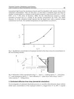
further insight into CRB can be gained by understanding how each IDS affects it. With the ar-
chitecture shown in Fig. 1, the model is given by
ˆ
s
=
∑
n
i
=1
w
i
s
i
. The bound is calculated from
the effective variance of each one of the IDSs as
ˆ
σ
2
i
=
σ
2
i
w
2
i
and then combining them to have the
CRB as
1
∑

n
i
=1
1
ˆ
σ
2
i
.
The weight assigned to the IDSs is inversely proportional to the variance. This is due to the
fact that, if the variance is small, the IDS is expected to be more dependable. The bound on
the smallest variance of an estimation
ˆ
s is given as:
ˆ
σ
2
= E[(
ˆ
s
−s)
2
] ≥
1
∑
n
i
=1
w
2

i
σ
2
i
(26)
It can be observed from equation 26 that any IDS decision that is not reliable will have a very
limited impact on the bound. This is because the non-reliable IDS will have a much larger
variance than other IDSs in the group;
ˆ
σ
2
n

ˆ
σ
2
1
,- - - ,
ˆ
σ
2
n
−1
and hence
1
ˆ
σ
2
n


1
ˆ
σ
2
1
, −- - ,
1
ˆ
σ
2
n
−1
. The
bound can then be approximated as
1
∑
n−1
i
=1
1
ˆ
σ
2
i
.
Also, it can be observed from equation 26 that the bound shows asymptotically optimum
behavior of minimum variance. Then,
ˆ
σ
2

i
> 0 and
ˆ
σ
2
min
= min[
ˆ
σ
2
i
, −− −,
ˆ
σ
2
n
], then
CRB
=
1
∑
n
i
=1
1
ˆ
σ
2
i
<

ˆ
σ
2
min
≤
ˆ
σ
2
i
(27)
From equation 27 it can also be shown that perfect performance is apparently possible with
enough IDSs. The bound tends to zero as more and more individual IDSs are added to the
fusion unit.
CRB
n→∞
= Lt
n→∞
1
1
ˆ
σ
2
1
+ − −− +
1
ˆ
σ
2
n
(28)

Mathematical Basis of Sensor Fusion in Intrusion Detection Systems 239
estimated and
ˆ
s to be the estimate of the fusion output. In most cases the estimate is a deter-
ministic function of the data. Then the mean square error (MSE) associated with the estimate
ˆ
s for a particular test data set is given as E
[(s −
ˆ
s
)
2
]. For a given value of s, there are two basic
kinds of errors:
. Random error, which is also called precision or estimation variance.
. Systematic error, which is also called accuracy or estimation bias.
Both kinds of errors can be quantiﬁed by the conditional distribution of the estimates pr
(
ˆ
s
−s).
The MSE of a detector is the expected value of the error and is due to the randomness or due
to the estimator not taking into account the information that could produce a more accurate
result.
MSE
= E[(s −
ˆ
s
)
2

] = Var(
ˆ
s
) + (Bias(
ˆ
s, s
))
2
(22)
The MSE is the absolute error used to assess the quality of the sensor in terms of its variation
and unbiasedness. For an unbiased sensor, the M SE is the variance of the estimator, or the
root mean squared error
(RMSE) is the standard deviation. The standard deviation measures
the accuracy of a set of probability assessments. The lower the value of RMSE, the better it is
as an estimator in terms of both the precision as well as the accuracy. Thus, reduced variance
can be considered as an index of improved accuracy and precision of any detector. Hence, the
reduction in variance of the fusion IDS to show its improved performance is proved in this
chapter. The Cramer-Rao inequality can be used for deriving the lower bound on the variance
of an estimator.
Cramer-Rao Bound (CRB) for fused output
The Cramer-Rao lower bound is used to get the best achievable estimation performance. Any
sensor fusion approach which achieves this performance is optimum in this regard. CR in-
equality states that the reciprocal of the Fisher information is an asymptotic lower bound on
the variance of any unbiased estimator
ˆ
s. Fisher information is a method for summarizing the
inﬂuence of the parameters of a generative model on a collection of samples from that model.
In this case, the parameters we consider are the means of the Gaussians. Fisher information is
the variance, (σ
2

) of the score (partial derivative of the logarithm of the likelihood function of
the network trafﬁc with respect to σ
2
).
score
=
∂
∂σ
2
ln(L(σ
2
; s)) (23)
Basically, the score tells us how sensitive the log-likelihood is to changes in parameters. This is
a function of variance, σ
2
and the detection s and this score is a sufﬁcient statistic for variance.
The expected value of this score is zero, and hence the Fisher information is given by:
E

[
∂
∂σ
2
ln(L(σ
2
; s))]
2
|σ
2


(24)
Fisher information is thus the expectation of the squared score. A random variable carrying
high Fisher information implies that the absolute value of the score is often high.
Cramer-Rao inequality expresses a lower bound on the variance of an unbiased statistical
estimator, based on the Fisher information.
σ
2
≥
1
F isher inf ormation
=
1
E

[
∂
∂σ
2
ln(L(σ
2
; X))]
2
|σ
2

(25)
If the prior probability of detection of the various IDSs are known, the weights w
i
|i=1,−−−n
can

be assigned to the individual IDSs. The idea is to estimate the local accuracy of the IDSs. The
decision of the IDS with the highest local accuracy estimate will have the highest weighting
on aggregation. The best fusion algorithm is supposed to choose the correct class if any of the
individual IDS did so. This is a theoretical upper bound for all fusion algorithms. Of course,
the best individual IDS is a lower bound for any meaningful fusion algorithm. Depending
on the data, the fusion may sometimes be no better than Bayes. In such cases, the upper and
lower performance bounds are identical and there is no point in using a fusion algorithm. A
further insight into CRB can be gained by understanding how each IDS affects it. With the ar-
chitecture shown in Fig. 1, the model is given by
ˆ
s
=
∑
n
i
=1
w
i
s
i
. The bound is calculated from
the effective variance of each one of the IDSs as
ˆ
σ
2
i
=
σ
2
i

w
2
i
and then combining them to have the
CRB as
1
∑
n
i
=1
1
ˆ
σ
2
i
.
The weight assigned to the IDSs is inversely proportional to the variance. This is due to the
fact that, if the variance is small, the IDS is expected to be more dependable. The bound on
the smallest variance of an estimation
ˆ
s is given as:
ˆ
σ
2
= E[(
ˆ
s
−s)
2
] ≥

1
∑
n
i
=1
w
2
i
σ
2
i
(26)
It can be observed from equation 26 that any IDS decision that is not reliable will have a very
limited impact on the bound. This is because the non-reliable IDS will have a much larger
variance than other IDSs in the group;
ˆ
σ
2
n

ˆ
σ
2
1
,- - - ,
ˆ
σ
2
n
−1

and hence
1
ˆ
σ
2
n

1
ˆ
σ
2
1
, −- - ,
1
ˆ
σ
2
n
−1
. The
bound can then be approximated as
1
∑
n−1
i
=1
1
ˆ
σ
2

i
.
Also, it can be observed from equation 26 that the bound shows asymptotically optimum
behavior of minimum variance. Then,
ˆ
σ
2
i
> 0 and
ˆ
σ
2
min
= min[
ˆ
σ
2
i
, −− −,
ˆ
σ
2
n
], then
CRB
=
1
∑
n
i

=1
1
ˆ
σ
2
i
<
ˆ
σ
2
min
≤
ˆ
σ
2
i
(27)
From equation 27 it can also be shown that perfect performance is apparently possible with
enough IDSs. The bound tends to zero as more and more individual IDSs are added to the
fusion unit.
CRB
n→∞
= Lt
n→∞
1
1
ˆ
σ
2
1

+ − −− +
1
ˆ
σ
2
n
(28)
Sensor Fusion and Its Applications240
For simplicity assume homogeneous IDSs with variance
ˆ
σ
2
;
CRB
n→∞
= Lt
n→∞
1
n
ˆ
σ
2
= Lt
n→∞
ˆ
σ
2
n
= 0 (29)
From equation 28 and equation 29 it can be easily interpreted that increasing the number

of IDSs to a sufﬁciently large number will lead to the performance bounds towards perfect
estimates. Also, due to monotone decreasing nature of the bound, the IDSs can be chosen to
make the performance as close to perfect.
4.2.2 Fusion of Dependent Sensors
In most of the sensor fusion problems, individual sensor errors are assumed to be uncorre-
lated so that the sensor decisions are independent. While independence of sensors is a good
assumption, it is often unrealistic in the normal case.
Setting bounds on false positives and true positives
As an illustration, let us consider a system with three individual IDSs, with a joint density at
the IDSs having a covariance matrix of the form:

=


1 ρ
12
ρ
13
ρ
21
1 ρ
23
ρ
31
ρ
32
1


(30)

The false alarm rate (α) at the fusion center, where the individual decisions are aggregated can
be written as:
α
max
= 1 − Pr(s
1
= 0, s
2
= 0, s
3
= 0|normal) = 1 −

t
−∞

t
−∞

t
−∞
P
s
(s|normal)ds (31)
where P
s
(s|normal) is the density of the sensor observations under the hypothesis normal
and is a function of the correlation coefﬁcient, ρ. Assuming a single threshold, T, for all the
sensors, and with the same correlation coefﬁcient, ρ between different sensors, a function
F
n

(T|ρ) = Pr(s
1
= 0, s
2
= 0, s
3
= 0) can be deﬁned.
F
n
(T|ρ) =

−∞
−∞
F
n
(
T −
√
ρy

1 − ρ
) f(y)dy (32)
where f
(y) and F(X) are the standard normal density and cumulative distribution function
respectively.
F
n
(X) = [F(X)]
n
Equation 31 can be written depending on whether ρ >

−1
n−1
or not, as:
α
max
= 1 −

∞
−∞
F
3
(
T −
√
ρy

1 − ρ
) f(y)dy f or 0 ≤ ρ < 1 (33)
and
α
max
= 1 − F
3
(T |ρ) f or −0.5 ≤ ρ < 1 (34)
With this threshold T, the probability of detection at the fusion unit can be computed as:
TP
min
= 1 −

∞

−∞
F
3
(
T −S −
√
ρy

1
−ρ
) f(y)dy f or 0 ≤ ρ < 1 (35)
and
TP
min
= 1 − F
3
(T − S |ρ) f or − 0.5 ≤ ρ < 1 (36)
The above equations 33, 34, 35, and 36, clearly showed the performance improvement of sen-
sor fusion where the upper bound on false positive rate and lower bound on detection rate
were ﬁxed. The system performance was shown to deteriorate when the correlation between
the sensor errors was positive and increasing, while the performance improved considerably
when the correlation was negative and increasing.
The above analysis were made with the assumption that the prior detection probability of
the individual IDSs were known and hence the case of bounded variance. However, in case
the IDS performance was not known a priori, it was a case of unbounded variance and hence
given the trivial model it was difﬁcult to accuracy estimate the underlying decision. This
clearly emphasized the difﬁculty of sensor fusion problem, where it becomes a necessity to
understand the individual IDS behavior. Hence the architecture was modiﬁed as proposed in
the work of Thomas & Balakrishnan (2008) and shown in Fig. 2 with the model remaining the
same. With this improved architecture using a neural network learner, a clear understanding

of each one of the individual IDSs was obtained. Most other approaches treat the training
data as a monolithic whole when determining the sensor accuracy. However, the accuracy
was expected to vary with data. This architecture attempts to predict the IDSs that are reliable
for a given sample data. This architecture is demonstrated to be practically successful and is
also the true situation where the weights are neither completely known nor totally unknown.
Fig. 2. Data-Dependent Decision Fusion architecture
4.3 Data-Dependent Decision Fusion Scheme
It is necessary to incorporate an architecture that considers a method for improving the detec-
tion rate by gathering an in-depth understanding on the input trafﬁc and also on the behavior
of the individual IDSs. This helps in automatically learning the individual weights for the
Mathematical Basis of Sensor Fusion in Intrusion Detection Systems 241
For simplicity assume homogeneous IDSs with variance
ˆ
σ
2
;
CRB
n→∞
= Lt
n→∞
1
n
ˆ
σ
2
= Lt
n→∞
ˆ
σ
2

n
= 0 (29)
From equation 28 and equation 29 it can be easily interpreted that increasing the number
of IDSs to a sufﬁciently large number will lead to the performance bounds towards perfect
estimates. Also, due to monotone decreasing nature of the bound, the IDSs can be chosen to
make the performance as close to perfect.
4.2.2 Fusion of Dependent Sensors
In most of the sensor fusion problems, individual sensor errors are assumed to be uncorre-
lated so that the sensor decisions are independent. While independence of sensors is a good
assumption, it is often unrealistic in the normal case.
Setting bounds on false positives and true positives
As an illustration, let us consider a system with three individual IDSs, with a joint density at
the IDSs having a covariance matrix of the form:

=


1 ρ
12
ρ
13
ρ
21
1 ρ
23
ρ
31
ρ
32
1



(30)
The false alarm rate (α) at the fusion center, where the individual decisions are aggregated can
be written as:
α
max
= 1 − Pr(s
1
= 0, s
2
= 0, s
3
= 0|normal) = 1 −

t
−∞

t
−∞

t
−∞
P
s
(s|normal)ds (31)
where P
s
(s|normal) is the density of the sensor observations under the hypothesis normal
and is a function of the correlation coefﬁcient, ρ. Assuming a single threshold, T, for all the

sensors, and with the same correlation coefﬁcient, ρ between different sensors, a function
F
n
(T|ρ) = Pr(s
1
= 0, s
2
= 0, s
3
= 0) can be deﬁned.
F
n
(T|ρ) =

−∞
−∞
F
n
(
T −
√
ρy

1
−ρ
) f(y)dy (32)
where f
(y) and F(X) are the standard normal density and cumulative distribution function
respectively.
F

n
(X) = [F(X)]
n
Equation 31 can be written depending on whether ρ >
−1
n
−1
or not, as:
α
max
= 1 −

∞
−∞
F
3
(
T −
√
ρy

1
−ρ
) f(y)dy f or 0 ≤ ρ < 1 (33)
and
α
max
= 1 − F
3
(T |ρ) f or −0.5 ≤ ρ < 1 (34)

With this threshold T, the probability of detection at the fusion unit can be computed as:
TP
min
= 1 −

∞
−∞
F
3
(
T −S −
√
ρy

1 − ρ
) f(y)dy f or 0 ≤ ρ < 1 (35)
and
TP
min
= 1 − F
3
(T − S |ρ) f or − 0.5 ≤ ρ < 1 (36)
The above equations 33, 34, 35, and 36, clearly showed the performance improvement of sen-
sor fusion where the upper bound on false positive rate and lower bound on detection rate
were ﬁxed. The system performance was shown to deteriorate when the correlation between
the sensor errors was positive and increasing, while the performance improved considerably
when the correlation was negative and increasing.
The above analysis were made with the assumption that the prior detection probability of
the individual IDSs were known and hence the case of bounded variance. However, in case
the IDS performance was not known a priori, it was a case of unbounded variance and hence

given the trivial model it was difﬁcult to accuracy estimate the underlying decision. This
clearly emphasized the difﬁculty of sensor fusion problem, where it becomes a necessity to
understand the individual IDS behavior. Hence the architecture was modiﬁed as proposed in
the work of Thomas & Balakrishnan (2008) and shown in Fig. 2 with the model remaining the
same. With this improved architecture using a neural network learner, a clear understanding
of each one of the individual IDSs was obtained. Most other approaches treat the training
data as a monolithic whole when determining the sensor accuracy. However, the accuracy
was expected to vary with data. This architecture attempts to predict the IDSs that are reliable
for a given sample data. This architecture is demonstrated to be practically successful and is
also the true situation where the weights are neither completely known nor totally unknown.
Fig. 2. Data-Dependent Decision Fusion architecture
4.3 Data-Dependent Decision Fusion Scheme
It is necessary to incorporate an architecture that considers a method for improving the detec-
tion rate by gathering an in-depth understanding on the input trafﬁc and also on the behavior
of the individual IDSs. This helps in automatically learning the individual weights for the
Sensor Fusion and Its Applications242
combination when the IDSs are heterogeneous and shows difference in performance. The ar-
chitecture should be independent of the dataset and the structures employed, and has to be
used with any real valued data set.
A new data-dependent architecture underpinning sensor fusion to signiﬁcantly enhance the
IDS performance is attempted in the work of Thomas & Balakrishnan (2008; 2009). A bet-
ter architecture by explicitly introducing the data-dependence in the fusion technique is the
key idea behind this architecture. The disadvantage of the commonly used fusion techniques
which are either implicitly data-dependent or data-independent, is due to the unrealistic con-
ﬁdence of certain IDSs. The idea in this architecture is to properly analyze the data and un-
derstand when the individual IDSs fail. The fusion unit should incorporate this learning from
input as well as from the output of detectors to make an appropriate decision. The fusion
should thus be data-dependent and hence the rule set has to be developed dynamically. This
architecture is different from conventional fusion architectures and guarantees improved per-
formance in terms of detection rate and the false alarm rate. It works well even for large

datasets and is capable of identifying novel attacks since the rules are dynamically updated.
It also has the advantage of improved scalability.
The Data-dependent Decision fusion architecture has three-stages; the IDSs that produce the
alerts as the ﬁrst stage, the neural network supervised learner determining the weights to the
IDSs’ decisions depending on the input as the second stage, and then the fusion unit doing
the weighted aggregation as the ﬁnal stage. The neural network learner can be considered as
a pre-processing stage to the fusion unit. The neural network is most appropriate for weight
determination, since it becomes difﬁcult to deﬁne the rules clearly, mainly as more number of
IDSs are added to the fusion unit. When a record is correctly classiﬁed by one or more detec-
tors, the neural network will accumulate this knowledge as a weight and with more number
of iterations, the weight gets stabilized. The architecture is independent of the dataset and the
structures employed, and can be used with any real valued dataset. Thus it is reasonable to
make use of a neural network learner unit to understand the performance and assign weights
to various individual IDSs in the case of a large dataset.
The weight assigned to any IDS not only depends on the output of that IDS as in the case
of the probability theory or the Dempster-Shafer theory, but also on the input trafﬁc which
causes this output. A neural network unit is fed with the output of the IDSs along with the
respective input for an in-depth understanding of the reliability estimation of the IDSs. The
alarms produced by the different IDSs when they are presented with a certain attack clearly
tell which sensor generated more precise result and what attacks are actually occurring on the
network trafﬁc. The output of the neural network unit corresponds to the weights which are
assigned to each one of the individual IDSs. The IDSs can be fused with the weight factor to
produce an improved resultant output.
This architecture refers to a collection of diverse IDSs that respond to an input trafﬁc and the
weighted combination of their predictions. The weights are learned by looking at the response
of the individual sensors for every input trafﬁc connection. The fusion output is represented
as:
s
= F
j

(w
i
j
(x
j
, s
i
j
), s
i
j
), (37)
where the weights w
i
j
are dependent on both the input x
j
as well as individual IDS’s output
s
i
j
, where the sufﬁx j refers to the class label and the preﬁx i refers to the IDS index. The fusion
unit used gives a value of one or zero depending on the set threshold being higher or lower
than the weighted aggregation of the IDS’s decisions.
The training of the neural network unit by back propagation involves three stages: 1) the feed
forward of the output of all the IDSs along with the input training pattern, which collectively
form the training pattern for the neural network learner unit, 2) the calculation and the back
propagation of the associated error, and 3) the adjustments of the weights. After the training,
the neural network is used for the computations of the feedforward phase. A multilayer net-
work with a single hidden layer is sufﬁcient in our application to learn the reliability of the

IDSs to an arbitrary accuracy according to the proof available in Fausett (2007).
Consider the problem formulation where the weights w
1
, , w
n
, take on constrained values
to satisfy the condition
∑
n
i
=1
w
i
= 1. Even without any knowledge about the IDS selectivity
factors, the constraint on the weights assures the possibility to accuracy estimate the underly-
ing decision. With the weights learnt for any data, it becomes a useful generalization of the
trivial model which was initially discussed. The improved efﬁcient model with good learning
algorithm can be used to ﬁnd the optimum fusion algorithms for any performance measure.
5. Results and Discussion
This section includes the empirical evaluation to support the theoretical analysis on the ac-
ceptability of sensor fusion in intrusion detection.
5.1 Data Set
The proposed fusion IDS was evaluated on two data, one being the real-world network traf-
ﬁc embedded with attacks and the second being the DARPA-1999 (1999). The real trafﬁc
within a protected University campus network was collected during the working hours of a
day. This trafﬁc of around two million packets was divided into two halves, one for training
the anomaly IDSs, and the other for testing. The test data was injected with 45 HTTP attack
packets using the HTTP attack trafﬁc generator tool called libwhisker Libwhisker (n.d.). The
test data set was introduced with a base rate of 0.0000225, which is relatively realistic. The
MIT Lincoln Laboratory under DARPA and AFRL sponsorship, has collected and distributed

the ﬁrst standard corpora for evaluation of computer network IDSs. This MIT- DARPA-1999
(1999) was used to train and test the performance of IDSs. The data for the weeks one and
three were used for the training of the anomaly detectors and the weeks four and ﬁve were
used as the test data. The training of the neural network learner was performed on the train-
ing data for weeks one, two and three, after the individual IDSs were trained. Each of the
IDS was trained on distinct portions of the training data (ALAD on week one and PHAD on
week three), which is expected to provide independence among the IDSs and also to develop
diversity while being trained.
The classiﬁcation of the various attacks found in the network trafﬁc is explained in detail in the
thesis work of Kendall (1999) with respect to DARPA intrusion detection evaluation dataset
and is explained here in brief. The attacks fall into four main classes namely, Probe, Denial
of Service(DoS), Remote to Local(R2L) and the User to Root (U2R). The Probe or Scan attacks
Mathematical Basis of Sensor Fusion in Intrusion Detection Systems 243
combination when the IDSs are heterogeneous and shows difference in performance. The ar-
chitecture should be independent of the dataset and the structures employed, and has to be
used with any real valued data set.
A new data-dependent architecture underpinning sensor fusion to signiﬁcantly enhance the
IDS performance is attempted in the work of Thomas & Balakrishnan (2008; 2009). A bet-
ter architecture by explicitly introducing the data-dependence in the fusion technique is the
key idea behind this architecture. The disadvantage of the commonly used fusion techniques
which are either implicitly data-dependent or data-independent, is due to the unrealistic con-
ﬁdence of certain IDSs. The idea in this architecture is to properly analyze the data and un-
derstand when the individual IDSs fail. The fusion unit should incorporate this learning from
input as well as from the output of detectors to make an appropriate decision. The fusion
should thus be data-dependent and hence the rule set has to be developed dynamically. This
architecture is different from conventional fusion architectures and guarantees improved per-
formance in terms of detection rate and the false alarm rate. It works well even for large
datasets and is capable of identifying novel attacks since the rules are dynamically updated.
It also has the advantage of improved scalability.
The Data-dependent Decision fusion architecture has three-stages; the IDSs that produce the

alerts as the ﬁrst stage, the neural network supervised learner determining the weights to the
IDSs’ decisions depending on the input as the second stage, and then the fusion unit doing
the weighted aggregation as the ﬁnal stage. The neural network learner can be considered as
a pre-processing stage to the fusion unit. The neural network is most appropriate for weight
determination, since it becomes difﬁcult to deﬁne the rules clearly, mainly as more number of
IDSs are added to the fusion unit. When a record is correctly classiﬁed by one or more detec-
tors, the neural network will accumulate this knowledge as a weight and with more number
of iterations, the weight gets stabilized. The architecture is independent of the dataset and the
structures employed, and can be used with any real valued dataset. Thus it is reasonable to
make use of a neural network learner unit to understand the performance and assign weights
to various individual IDSs in the case of a large dataset.
The weight assigned to any IDS not only depends on the output of that IDS as in the case
of the probability theory or the Dempster-Shafer theory, but also on the input trafﬁc which
causes this output. A neural network unit is fed with the output of the IDSs along with the
respective input for an in-depth understanding of the reliability estimation of the IDSs. The
alarms produced by the different IDSs when they are presented with a certain attack clearly
tell which sensor generated more precise result and what attacks are actually occurring on the
network trafﬁc. The output of the neural network unit corresponds to the weights which are
assigned to each one of the individual IDSs. The IDSs can be fused with the weight factor to
produce an improved resultant output.
This architecture refers to a collection of diverse IDSs that respond to an input trafﬁc and the
weighted combination of their predictions. The weights are learned by looking at the response
of the individual sensors for every input trafﬁc connection. The fusion output is represented
as:
s
= F
j
(w
i
j

(x
j
, s
i
j
), s
i
j
), (37)
where the weights w
i
j
are dependent on both the input x
j
as well as individual IDS’s output
s
i
j
, where the sufﬁx j refers to the class label and the preﬁx i refers to the IDS index. The fusion
unit used gives a value of one or zero depending on the set threshold being higher or lower
than the weighted aggregation of the IDS’s decisions.
The training of the neural network unit by back propagation involves three stages: 1) the feed
forward of the output of all the IDSs along with the input training pattern, which collectively
form the training pattern for the neural network learner unit, 2) the calculation and the back
propagation of the associated error, and 3) the adjustments of the weights. After the training,
the neural network is used for the computations of the feedforward phase. A multilayer net-
work with a single hidden layer is sufﬁcient in our application to learn the reliability of the
IDSs to an arbitrary accuracy according to the proof available in Fausett (2007).
Consider the problem formulation where the weights w
1

, , w
n
, take on constrained values
to satisfy the condition
∑
n
i
=1
w
i
= 1. Even without any knowledge about the IDS selectivity
factors, the constraint on the weights assures the possibility to accuracy estimate the underly-
ing decision. With the weights learnt for any data, it becomes a useful generalization of the
trivial model which was initially discussed. The improved efﬁcient model with good learning
algorithm can be used to ﬁnd the optimum fusion algorithms for any performance measure.
5. Results and Discussion
This section includes the empirical evaluation to support the theoretical analysis on the ac-
ceptability of sensor fusion in intrusion detection.
5.1 Data Set
The proposed fusion IDS was evaluated on two data, one being the real-world network traf-
ﬁc embedded with attacks and the second being the DARPA-1999 (1999). The real trafﬁc
within a protected University campus network was collected during the working hours of a
day. This trafﬁc of around two million packets was divided into two halves, one for training
the anomaly IDSs, and the other for testing. The test data was injected with 45 HTTP attack
packets using the HTTP attack trafﬁc generator tool called libwhisker Libwhisker (n.d.). The
test data set was introduced with a base rate of 0.0000225, which is relatively realistic. The
MIT Lincoln Laboratory under DARPA and AFRL sponsorship, has collected and distributed
the ﬁrst standard corpora for evaluation of computer network IDSs. This MIT- DARPA-1999
(1999) was used to train and test the performance of IDSs. The data for the weeks one and
three were used for the training of the anomaly detectors and the weeks four and ﬁve were

used as the test data. The training of the neural network learner was performed on the train-
ing data for weeks one, two and three, after the individual IDSs were trained. Each of the
IDS was trained on distinct portions of the training data (ALAD on week one and PHAD on
week three), which is expected to provide independence among the IDSs and also to develop
diversity while being trained.
The classiﬁcation of the various attacks found in the network trafﬁc is explained in detail in the
thesis work of Kendall (1999) with respect to DARPA intrusion detection evaluation dataset
and is explained here in brief. The attacks fall into four main classes namely, Probe, Denial
of Service(DoS), Remote to Local(R2L) and the User to Root (U2R). The Probe or Scan attacks
Sensor Fusion and Its Applications244
automatically scan a network of computers or a DNS server to ﬁnd valid IP addresses, active
ports, host operating system types and known vulnerabilities. The DoS attacks are designed
to disrupt a host or network service. In R2L attacks, an attacker who does not have an account
on a victim machine gains local access to the machine, exﬁltrates ﬁles from the machine or
modiﬁes data in transit to the machine. In U2R attacks, a local user on a machine is able to
obtain privileges normally reserved for the unix super user or the windows administrator.
Even with the criticisms by McHugh (2000) and Mahoney & Chan (2003) against the DARPA
dataset, the dataset was extremely useful in the IDS evaluation undertaken in this work. Since
none of the IDSs perform exceptionally well on the DARPA dataset, the aim is to show that
the performance improves with the proposed method. If a system is evaluated on the DARPA
dataset, then it cannot claim anything more in terms of its performance on the real network
trafﬁc. Hence this dataset can be considered as the base line of any research Thomas & Balakr-
ishnan (2007). Also, even after ten years of its generation, even now there are lot of attacks in
the dataset for which signatures are not available in database of even the frequently updated
signature based IDSs like Snort (1999). The real data trafﬁc is difﬁcult to work with; the main
reason being the lack of the information regarding the status of the trafﬁc. Even with intense
analysis, the prediction can never be 100 percent accurate because of the stealthiness and so-
phistication of the attacks and the unpredictability of the non-malicious user as well as the
intricacies of the users in general.
5.2 Test Setup

The test set up for experimental evaluation consisted of three Pentium machines with Linux
Operating System. The experiments were conducted with IDSs, PHAD (2001), ALAD (2002),
and Snort (1999), distributed across the single subnet observing the same domain. PHAD, is
based on attack detection by extracting the packet header information, whereas ALAD is ap-
plication payload-based, and Snort detects by collecting information from both the header and
the payload part of every packet on time-based as well as on connection-based manner. This
choice of heterogeneous sensors in terms of their functionality was to exploit the advantages
of fusion IDS Bass (1999). The PHAD being packet-header based and detecting one packet
at a time, was totally unable to detect the slow scans. However, PHAD detected the stealthy
scans much more effectively. The ALAD being content-based has complemented the PHAD
by detecting the Remote to Local (R2L) and the User to Root (U2R) with appreciable efﬁciency.
Snort was efﬁcient in detecting the Probes as well as the DoS attacks.
The weight analysis of the IDS data coming from PHAD, ALAD, and Snort was carried out by
the Neural Network supervised learner before it was fed to the fusion element. The detectors
PHAD and ALAD produces the IP address along with the anomaly score whereas the Snort
produces the IP address along with severity score of the alert. The alerts produced by these
IDSs are converted to a standard binary form. The Neural Network learner inputs these deci-
sions along with the particular trafﬁc input which was monitored by the IDSs.
The neural network learner was designed as a feed forward back propagation algorithm with
a single hidden layer and 25 sigmoidal hidden units in the hidden layer. Experimental proof
is available for the best performance of the Neural Network with the number of hidden units
being log
(T), where T is the number of training samples in the dataset Lippmann (1987). The
values chosen for the initial weights lie in the range of
−0.5 to 0.5 and the ﬁnal weights after
training may also be of either sign. The learning rate is chosen to be 0.02. In order to train the
neural network, it is necessary to expose them to both normal and anomalous data. Hence,
during the training, the network was exposed to weeks 1, 2, and 3 of the training data and the
weights were adjusted using the back propagation algorithm. An epoch of training consisted
of one pass over the training data. The training proceeded until the total error made during

each epoch stopped decreasing or 1000 epochs had been reached. If the neural network stops
learning before reaching an acceptable solution, a change in the number of hidden nodes or in
the learning parameters will often ﬁx the problem. The other possibility is to start over again
with a different set of initial weights.
The fusion unit performed the weighted aggregation of the IDS outputs for the purpose of
identifying the attacks in the test dataset. It used binary fusion by giving an output value of
one or zero depending the value of the weighted aggregation of the various IDS decisions.
The packets were identiﬁed by their timestamp on aggregation. A value of one at the output
of the fusion unit indicated the record to be under attack and a zero indicated the absence of
an attack.
5.3 Metrics for Performance Evaluation
The detection accuracy is calculated as the proportion of correct detections. This traditional
evaluation metric of detection accuracy was not adequate while dealing with classes like U2R
and R2L which are very rare. The cost matrix published in KDD’99 Elkan (2000) to measure
the damage of misclassiﬁcation, highlights the importance of these two rare classes. Majority
of the existing IDSs have ignored these rare classes, since it will not affect the detection accu-
racy appreciably. The importance of these rare classes is overlooked by most of the IDSs with
the metrics commonly used for evaluation namely the false positive rate and the detection
rate.
5.3.1 ROC and AUC
ROC curves are used to evaluate IDS performance over a range of trade-offs between detec-
tion rate and the false positive rate. The Area Under ROC Curve (AUC) is a convenient way
of comparing IDSs. AUC is the performance metric for the ROC curve.
5.3.2 Precision, Recall and F-score
Precision (P) is a measure of what fraction of the test data detected as attack are actually from
the attack class. Recall (R) on the other hand is a measure of what fraction of attack class is
correctly detected. There is a natural trade-off between the metrics precision and recall. It
is required to evaluate any IDS based on how it performs on both recall and precision. The
metric used for this purpose is F-score, which ranges from [0,1]. The F-score can be considered
as the harmonic mean of recall and precision, given by:

F-score
=
2 ∗ P ∗R
P + R
(38)
Higher value of F-score indicates that the IDS is performing better on recall as well as preci-
sion.
Mathematical Basis of Sensor Fusion in Intrusion Detection Systems 245
automatically scan a network of computers or a DNS server to ﬁnd valid IP addresses, active
ports, host operating system types and known vulnerabilities. The DoS attacks are designed
to disrupt a host or network service. In R2L attacks, an attacker who does not have an account
on a victim machine gains local access to the machine, exﬁltrates ﬁles from the machine or
modiﬁes data in transit to the machine. In U2R attacks, a local user on a machine is able to
obtain privileges normally reserved for the unix super user or the windows administrator.
Even with the criticisms by McHugh (2000) and Mahoney & Chan (2003) against the DARPA
dataset, the dataset was extremely useful in the IDS evaluation undertaken in this work. Since
none of the IDSs perform exceptionally well on the DARPA dataset, the aim is to show that
the performance improves with the proposed method. If a system is evaluated on the DARPA
dataset, then it cannot claim anything more in terms of its performance on the real network
trafﬁc. Hence this dataset can be considered as the base line of any research Thomas & Balakr-
ishnan (2007). Also, even after ten years of its generation, even now there are lot of attacks in
the dataset for which signatures are not available in database of even the frequently updated
signature based IDSs like Snort (1999). The real data trafﬁc is difﬁcult to work with; the main
reason being the lack of the information regarding the status of the trafﬁc. Even with intense
analysis, the prediction can never be 100 percent accurate because of the stealthiness and so-
phistication of the attacks and the unpredictability of the non-malicious user as well as the
intricacies of the users in general.
5.2 Test Setup
The test set up for experimental evaluation consisted of three Pentium machines with Linux
Operating System. The experiments were conducted with IDSs, PHAD (2001), ALAD (2002),

and Snort (1999), distributed across the single subnet observing the same domain. PHAD, is
based on attack detection by extracting the packet header information, whereas ALAD is ap-
plication payload-based, and Snort detects by collecting information from both the header and
the payload part of every packet on time-based as well as on connection-based manner. This
choice of heterogeneous sensors in terms of their functionality was to exploit the advantages
of fusion IDS Bass (1999). The PHAD being packet-header based and detecting one packet
at a time, was totally unable to detect the slow scans. However, PHAD detected the stealthy
scans much more effectively. The ALAD being content-based has complemented the PHAD
by detecting the Remote to Local (R2L) and the User to Root (U2R) with appreciable efﬁciency.
Snort was efﬁcient in detecting the Probes as well as the DoS attacks.
The weight analysis of the IDS data coming from PHAD, ALAD, and Snort was carried out by
the Neural Network supervised learner before it was fed to the fusion element. The detectors
PHAD and ALAD produces the IP address along with the anomaly score whereas the Snort
produces the IP address along with severity score of the alert. The alerts produced by these
IDSs are converted to a standard binary form. The Neural Network learner inputs these deci-
sions along with the particular trafﬁc input which was monitored by the IDSs.
The neural network learner was designed as a feed forward back propagation algorithm with
a single hidden layer and 25 sigmoidal hidden units in the hidden layer. Experimental proof
is available for the best performance of the Neural Network with the number of hidden units
being log
(T), where T is the number of training samples in the dataset Lippmann (1987). The
values chosen for the initial weights lie in the range of
−0.5 to 0.5 and the ﬁnal weights after
training may also be of either sign. The learning rate is chosen to be 0.02. In order to train the
neural network, it is necessary to expose them to both normal and anomalous data. Hence,
during the training, the network was exposed to weeks 1, 2, and 3 of the training data and the
weights were adjusted using the back propagation algorithm. An epoch of training consisted
of one pass over the training data. The training proceeded until the total error made during
each epoch stopped decreasing or 1000 epochs had been reached. If the neural network stops
learning before reaching an acceptable solution, a change in the number of hidden nodes or in

the learning parameters will often ﬁx the problem. The other possibility is to start over again
with a different set of initial weights.
The fusion unit performed the weighted aggregation of the IDS outputs for the purpose of
identifying the attacks in the test dataset. It used binary fusion by giving an output value of
one or zero depending the value of the weighted aggregation of the various IDS decisions.
The packets were identiﬁed by their timestamp on aggregation. A value of one at the output
of the fusion unit indicated the record to be under attack and a zero indicated the absence of
an attack.
5.3 Metrics for Performance Evaluation
The detection accuracy is calculated as the proportion of correct detections. This traditional
evaluation metric of detection accuracy was not adequate while dealing with classes like U2R
and R2L which are very rare. The cost matrix published in KDD’99 Elkan (2000) to measure
the damage of misclassiﬁcation, highlights the importance of these two rare classes. Majority
of the existing IDSs have ignored these rare classes, since it will not affect the detection accu-
racy appreciably. The importance of these rare classes is overlooked by most of the IDSs with
the metrics commonly used for evaluation namely the false positive rate and the detection
rate.
5.3.1 ROC and AUC
ROC curves are used to evaluate IDS performance over a range of trade-offs between detec-
tion rate and the false positive rate. The Area Under ROC Curve (AUC) is a convenient way
of comparing IDSs. AUC is the performance metric for the ROC curve.
5.3.2 Precision, Recall and F-score
Precision (P) is a measure of what fraction of the test data detected as attack are actually from
the attack class. Recall (R) on the other hand is a measure of what fraction of attack class is
correctly detected. There is a natural trade-off between the metrics precision and recall. It
is required to evaluate any IDS based on how it performs on both recall and precision. The
metric used for this purpose is F-score, which ranges from [0,1]. The F-score can be considered
as the harmonic mean of recall and precision, given by:
F-score
=

2 ∗ P ∗R
P + R
(38)
Higher value of F-score indicates that the IDS is performing better on recall as well as preci-
sion.
Sensor Fusion and Its Applications246
Attack type Total attacks Attacks detected % detection
Probe 37 22 59%
DoS 63 24 38%
R2L 53 6 11%
U2R/Data 37 2 5%
Total 190 54 28%
Table 1. Attacks of each type detected by PHAD at a false positive of 0.002%
Attack type Total attacks Attacks detected % detection
Probe 37 6 16%
DoS 63 19 30%
R2L 53 25 47%
U2R/Data 37 10 27%
Total 190 60 32%
Table 2. Attacks of each type detected by ALAD at a false positive of 0.002%
5.4 Experimental Evaluation
All the IDSs that form part of the fusion IDS were separately evaluated with the same two data
sets; 1) real-world trafﬁc and 2) the DARPA 1999 data set. Then the empirical evaluation of
the data-dependent decision fusion method was also observed. The results support the valid-
ity of the data-dependent approach compared to the various existing fusion methods of IDS.
It can be observed from tables 1, 2 and 3 that the attacks detected by different IDS were not
necessarily the same and also that no individual IDS was able to provide acceptable values of
all performance measures. It may be noted that the false alarm rates differ in the case of snort
as it was extremely difﬁcult to try for a fair comparison with equal false alarm rates for all the
IDSs because of the unacceptable ranges for the detection rate under such circumstances.

Table 4 and Fig. 3 show the improvement in performance of the Data-dependent Decision
fusion method over each of the three individual IDSs. The detection rate is acceptably high
for all types of attacks without affecting the false alarm rate.
The real trafﬁc within a protected University campus network was collected during the work-
ing hours of a day. This trafﬁc of around two million packets was divided into two halves,
one for training the anomaly IDSs, and the other for testing. The test data was injected with 45
HTTP attack packets using the HTTP attack trafﬁc generator tool called libwhisker Libwhisker
(n.d.). The test data set was introduced with a base rate of 0.0000225, which is relatively real-
istic. The comparison of the evaluated IDS with various other fusion techniques is illustrated
in table 5 with the real-world network trafﬁc.
The results evaluated in Table 6 show that the accuracy (Acc.) and AUC are not good met-
rics with the imbalanced data where the attack class is rare compared to the normal class.
Accuracy was heavily biased to favor majority class. Accuracy when used as a performance
measure assumed target class distribution to be known and unchanging, and the costs of FP
and FN to be equal. These assumptions are unrealistic. If metrics like accuracy and AUC are
to be used, then the data has to be more balanced in terms of the various classes. If AUC was
to be used as an evaluation metric a possible solution was to consider only the area under
Attack type Total attacks Attacks detected % detection
Probe 37 10 27%
DoS 63 30 48%
R2L 53 26 49%
U2R/Data 37 30 81%
Total 190 96 51%
Table 3. Attacks of each type detected by Snort at a false positive of 0.02%
Attack type Total attacks Attacks detected % detection
Probe 37 28 76%
DoS 63 40 64%
R2L 53 29 55%
U2R/Data 37 32 87%
Total 190 129 68%

Table 4. Attacks of each type detected by Data-dependent Decision Fusion architecture at a
false positive of 0.002%
the ROC curve until the FP-rate reaches the prior probability. The results presented in Table
5 indicate that the Data-dependent Decision fusion method performs signiﬁcantly better for
attack class with high recall as well as high precision as against achieving the high accuracy
alone.
The ROC Semilog curves of the individual IDSs and the DD fusion IDS are given in Fig.
4, which clearly show the better performance of the DD fusion method in comparison to the
three individual IDSs, PHAD, ALAD and Snort. The log-scale was used for the x-axis to iden-
tify the points which would otherwise be crowded on the x-axis.
Detector/ Total TP FP Precision Recall F-score
Fusion Type Attacks
PHAD 45 10 45 0.18 0.22 0.20
ALAD 45 18 45 0.29 0.4 0.34
Snort 45 11 400 0.03 0.24 0.05
OR 45 28 470 0.06 0.62 0.11
AND 45 8 29 0.22 0.18 0.20
SVM 45 23 94 0.2 0.51 0.29
ANN 45 25 131 0.16 0.56 0.25
Data-dependent 45 27 42 0.39 0.6 0.47
Decision Fusion
Table 5. Comparison of the evaluated IDSs with various evaluation metrics using the real-
world data set
Mathematical Basis of Sensor Fusion in Intrusion Detection Systems 247
Attack type Total attacks Attacks detected % detection
Probe 37 22 59%
DoS 63 24 38%
R2L 53 6 11%
U2R/Data 37 2 5%
Total 190 54 28%

Table 1. Attacks of each type detected by PHAD at a false positive of 0.002%
Attack type Total attacks Attacks detected % detection
Probe 37 6 16%
DoS 63 19 30%
R2L 53 25 47%
U2R/Data 37 10 27%
Total 190 60 32%
Table 2. Attacks of each type detected by ALAD at a false positive of 0.002%
5.4 Experimental Evaluation
All the IDSs that form part of the fusion IDS were separately evaluated with the same two data
sets; 1) real-world trafﬁc and 2) the DARPA 1999 data set. Then the empirical evaluation of
the data-dependent decision fusion method was also observed. The results support the valid-
ity of the data-dependent approach compared to the various existing fusion methods of IDS.
It can be observed from tables 1, 2 and 3 that the attacks detected by different IDS were not
necessarily the same and also that no individual IDS was able to provide acceptable values of
all performance measures. It may be noted that the false alarm rates differ in the case of snort
as it was extremely difﬁcult to try for a fair comparison with equal false alarm rates for all the
IDSs because of the unacceptable ranges for the detection rate under such circumstances.
Table 4 and Fig. 3 show the improvement in performance of the Data-dependent Decision
fusion method over each of the three individual IDSs. The detection rate is acceptably high
for all types of attacks without affecting the false alarm rate.
The real trafﬁc within a protected University campus network was collected during the work-
ing hours of a day. This trafﬁc of around two million packets was divided into two halves,
one for training the anomaly IDSs, and the other for testing. The test data was injected with 45
HTTP attack packets using the HTTP attack trafﬁc generator tool called libwhisker Libwhisker
(n.d.). The test data set was introduced with a base rate of 0.0000225, which is relatively real-
istic. The comparison of the evaluated IDS with various other fusion techniques is illustrated
in table 5 with the real-world network trafﬁc.
The results evaluated in Table 6 show that the accuracy (Acc.) and AUC are not good met-
rics with the imbalanced data where the attack class is rare compared to the normal class.

Accuracy was heavily biased to favor majority class. Accuracy when used as a performance
measure assumed target class distribution to be known and unchanging, and the costs of FP
and FN to be equal. These assumptions are unrealistic. If metrics like accuracy and AUC are
to be used, then the data has to be more balanced in terms of the various classes. If AUC was
to be used as an evaluation metric a possible solution was to consider only the area under
Attack type Total attacks Attacks detected % detection
Probe 37 10 27%
DoS 63 30 48%
R2L 53 26 49%
U2R/Data 37 30 81%
Total 190 96 51%
Table 3. Attacks of each type detected by Snort at a false positive of 0.02%
Attack type Total attacks Attacks detected % detection
Probe 37 28 76%
DoS 63 40 64%
R2L 53 29 55%
U2R/Data 37 32 87%
Total 190 129 68%
Table 4. Attacks of each type detected by Data-dependent Decision Fusion architecture at a
false positive of 0.002%
the ROC curve until the FP-rate reaches the prior probability. The results presented in Table
5 indicate that the Data-dependent Decision fusion method performs signiﬁcantly better for
attack class with high recall as well as high precision as against achieving the high accuracy
alone.
The ROC Semilog curves of the individual IDSs and the DD fusion IDS are given in Fig.
4, which clearly show the better performance of the DD fusion method in comparison to the
three individual IDSs, PHAD, ALAD and Snort. The log-scale was used for the x-axis to iden-
tify the points which would otherwise be crowded on the x-axis.
Detector/ Total TP FP Precision Recall F-score
Fusion Type Attacks

PHAD 45 10 45 0.18 0.22 0.20
ALAD 45 18 45 0.29 0.4 0.34
Snort 45 11 400 0.03 0.24 0.05
OR 45 28 470 0.06 0.62 0.11
AND 45 8 29 0.22 0.18 0.20
SVM 45 23 94 0.2 0.51 0.29
ANN 45 25 131 0.16 0.56 0.25
Data-dependent 45 27 42 0.39 0.6 0.47
Decision Fusion
Table 5. Comparison of the evaluated IDSs with various evaluation metrics using the real-
world data set
Sensor Fusion and Its Applications248
Fig. 3. Performance of Evaluated Systems
Detection/
Fusion P R Acc. AUC F-Score
PHAD 0.35 0.28 0.99 0.64 0.31
ALAD 0.38 0.32 0.99 0.66 0.35
Snort 0.09 0.51 0.99 0.75 0.15
Data-
Dependent 0.39 0.68 0.99 0.84 0.50
fusion
Table 6. Performance Comparison of individual IDSs and the Data-Dependent Fusion method
6. Conclusion
A discussion on the mathematical basis for sensor fusion in IDS is included in this chapter.
This study contributes to fusion ﬁeld in several aspects. Firstly, considering zero knowledge
about the detection systems and the trafﬁc data, an attempt is made to show the improved
performance of sensor fusion for intrusion detection application. The later half of the chapter
takes into account the analysis of the sensor fusion system with a knowledge of data and
sensors that are seen in practice. Independent as well as dependent detectors were considered
and the study clariﬁes the intuition that independence of detectors is crucial in determining

the success of fusion operation. If the individual sensors were complementary and looked
at different regions of the attack domain, then the data-dependent decision fusion enriches
the analysis on the incoming trafﬁc to detect attack with appreciably low false alarms. The
approach is tested with the standard DARPA IDS traces, and offers better performance than
any of the individual IDSs. The individual IDSs that are components of this architecture in
this particular work were PHAD, ALAD and Snort with detection rates 0.28, 0.32 and 0.51
respectively. Although the research discussed in this chapter has thus far focused on the three
10
−6
10
−5
10
−4
10
−3
10
−2
10
−1
10
0
0
0.1
0.2
0.3
0.4
0.5
0.6
0.7
0.8

0.9
1
FALSE POSITIVE RATE (LOG SCALE)
TRUE POSITIVE RATE
ROC SEMILOG CURVE
PHAD
ALAD
Snort
DD Fusion
Fig. 4. ROC Semilog curve of individual and combined IDSs
IDSs, namely, PHAD, ALAD and Snort, the algorithm works well with any IDS. The result
of the Data-dependent Decision fusion method is better than what has been predicted by the
Lincoln Laboratory after the DARPA IDS evaluation. An intrusion detection of 68% with a
false positive of as low as 0.002% is achieved using the DARPA data set and detection of 60%
with a false positive of as low as 0.002% is achieved using the real-world network trafﬁc. The
ﬁgure of merit, F-score of the data-dependent decision fusion method has improved to 0.50
for the DARPA data set and to 0.47 for the real-world network trafﬁc.
7. References
Aalo, V. & Viswanathan, R. (1995). On distributed detection with correlated sensors: Two
examples, IEEE Transactions on Aerospace and Electronic Systems Vol. 25(No. 3): 414–
421.
ALAD (2002). Learning non stationary models of normal network trafﬁc for detecting novel
attacks, SIGKDD.
Baek, W. & Bommareddy, S. (1995). Optimal m-ary data fusion with distributed sensors, IEEE
Transactions on Aerospace and Electronic Systems Vol. 31(No. 3): 1150–1152.
Bass, T. (1999). Multisensor data fusion for next generation distributed intrusion detection
systems, IRIS National Symposium.
Blum, R., Kassam, S. & Poor, H. (1995). Distributed detection with multiple sensors - part ii:
Advanced topics, Proceedings of IEEE pp. 64–79.
Brown, G. (2004). Diversity in neural network ensembles, PhD thesis .

Chair, Z. & Varshney, P. (1986). Optimal data fusion in multiple sensor detection systems,
IEEE Transactions on Aerospace and Electronic Systems Vol. 22(No. 1): 98–101.
DARPA-1999 (1999). />html.
Drakopoulos, E. & Lee, C. (1995). Optimum multisensor fusion of correlated local, IEEE Trans-
actions on Aerospace and Electronic Systems Vol. 27: 593–606.
Elkan, C. (2000). Results of the kdd’99 classiﬁer learning, SIGKDD Explorations, pp. 63–64.
Mathematical Basis of Sensor Fusion in Intrusion Detection Systems 249
Fig. 3. Performance of Evaluated Systems
Detection/
Fusion P R Acc. AUC F-Score
PHAD 0.35 0.28 0.99 0.64 0.31
ALAD 0.38 0.32 0.99 0.66 0.35
Snort 0.09 0.51 0.99 0.75 0.15
Data-
Dependent 0.39 0.68 0.99 0.84 0.50
fusion
Table 6. Performance Comparison of individual IDSs and the Data-Dependent Fusion method
6. Conclusion
A discussion on the mathematical basis for sensor fusion in IDS is included in this chapter.
This study contributes to fusion ﬁeld in several aspects. Firstly, considering zero knowledge
about the detection systems and the trafﬁc data, an attempt is made to show the improved
performance of sensor fusion for intrusion detection application. The later half of the chapter
takes into account the analysis of the sensor fusion system with a knowledge of data and
sensors that are seen in practice. Independent as well as dependent detectors were considered
and the study clariﬁes the intuition that independence of detectors is crucial in determining
the success of fusion operation. If the individual sensors were complementary and looked
at different regions of the attack domain, then the data-dependent decision fusion enriches
the analysis on the incoming trafﬁc to detect attack with appreciably low false alarms. The
approach is tested with the standard DARPA IDS traces, and offers better performance than
any of the individual IDSs. The individual IDSs that are components of this architecture in

this particular work were PHAD, ALAD and Snort with detection rates 0.28, 0.32 and 0.51
respectively. Although the research discussed in this chapter has thus far focused on the three
10
−6
10
−5
10
−4
10
−3
10
−2
10
−1
10
0
0
0.1
0.2
0.3
0.4
0.5
0.6
0.7
0.8
0.9
1
FALSE POSITIVE RATE (LOG SCALE)
TRUE POSITIVE RATE
ROC SEMILOG CURVE

PHAD
ALAD
Snort
DD Fusion
Fig. 4. ROC Semilog curve of individual and combined IDSs
IDSs, namely, PHAD, ALAD and Snort, the algorithm works well with any IDS. The result
of the Data-dependent Decision fusion method is better than what has been predicted by the
Lincoln Laboratory after the DARPA IDS evaluation. An intrusion detection of 68% with a
false positive of as low as 0.002% is achieved using the DARPA data set and detection of 60%
with a false positive of as low as 0.002% is achieved using the real-world network trafﬁc. The
ﬁgure of merit, F-score of the data-dependent decision fusion method has improved to 0.50
for the DARPA data set and to 0.47 for the real-world network trafﬁc.
7. References
Aalo, V. & Viswanathan, R. (1995). On distributed detection with correlated sensors: Two
examples, IEEE Transactions on Aerospace and Electronic Systems Vol. 25(No. 3): 414–
421.
ALAD (2002). Learning non stationary models of normal network trafﬁc for detecting novel
attacks, SIGKDD.
Baek, W. & Bommareddy, S. (1995). Optimal m-ary data fusion with distributed sensors, IEEE
Transactions on Aerospace and Electronic Systems Vol. 31(No. 3): 1150–1152.
Bass, T. (1999). Multisensor data fusion for next generation distributed intrusion detection
systems, IRIS National Symposium.
Blum, R., Kassam, S. & Poor, H. (1995). Distributed detection with multiple sensors - part ii:
Advanced topics, Proceedings of IEEE pp. 64–79.
Brown, G. (2004). Diversity in neural network ensembles, PhD thesis .
Chair, Z. & Varshney, P. (1986). Optimal data fusion in multiple sensor detection systems,
IEEE Transactions on Aerospace and Electronic Systems Vol. 22(No. 1): 98–101.
DARPA-1999 (1999). />html.
Drakopoulos, E. & Lee, C. (1995). Optimum multisensor fusion of correlated local, IEEE Trans-
actions on Aerospace and Electronic Systems Vol. 27: 593–606.

Elkan, C. (2000). Results of the kdd’99 classiﬁer learning, SIGKDD Explorations, pp. 63–64.
Sensor Fusion and Its Applications250
Fausett, L. (2007). My Life, Pearson Education.
Hall, D. H. & McMullen, S. A. H. (2000). Mathematical Techniques in Multi-Sensor Data Fusion,
Artech House.
Kam, M., Zhu, Q. & Gray, W. (1995). Optimal data fusion of correlated local decisions in mul-
tiple sensor detection systems, IEEE Transactions on Aerospace and Electronic Systems
Vol. 28: 916–920.
Kendall, K. (1999). A database of computer attacks for the evaluation of intrusion detection sytsems,
Thesis.
Krogh, A. & Vedelsby, J. (1995). Neural network ensembles, cross validation, and active learn-
ing, NIPS (No.7): 231–238.
Libwhisker (n.d.). /libwhisker.
Lippmann, R. (1987). An introduction to computing with neural nets, IEEE ASSP Magazine,
pp. 4–22.
Mahoney, M. & Chan, P. (2003). An analysis of the 1999 darpa /lincoln laboratory evaluation
data for network anomaly detection, Technical Report CS-2003-02, Publisher.
McHugh, J. (2000). Improvement in intrusion detection with advances in sensor fusion, ACM
Transactions on Information and System Security Vol. 3(4): 543–552.
Nahin, P. & Pokoski, J. (1980). Nctr plus sensor fusion equals iffn or can two plus two equal
ﬁve?, IEEE Transactions on Aerospace and Electronic Systems Vol. AES-16(No. 3): 320–
337.
PHAD (2001). Detecting novel attacks by identifying anomalous network packet headers,
Technical Report CS-2001-2.
Snort (1999). www.snort.org/docs/snort_htmanuals/htmanual_260.
Thomas, C. & Balakrishnan, N. (2007). Usefulness of darpa data set in intrusion detection
system evaluation, Proceedings of SPIE International Defense and Security Symposium.
Thomas, C. & Balakrishnan, N. (2008). Advanced sensor fusion technique for enhanced intru-
sion detection, Proceedings of IEEE International Conference on Intelligence and Security
Informatics, IEEE, Taiwan.

Thomas, C. & Balakrishnan, N. (2009). Improvement in intrusion detection with advances in
sensor fusion, IEEE Transactions on Information Forensics and Security Vol. 4(3): 543–
552.
Thomopoulos, S., Vishwanathan, R. & Bougoulias, D. (1987). Optimal decision fusion in mul-
tiple sensor systems, IEEE Transactions on Aerospace and Electronic Systems Vol. 23(No.
5): 644–651.
Sensor Fusion for Position Estimation in Networked Systems 251
Sensor Fusion for Position Estimation in Networked Systems
Giuseppe C. Calaore, Luca Carlone and MingzhuWei
0
Sensor Fusion for Position
Estimation in Networked Systems
Giuseppe C. Calaﬁore, Luca Carlone and Mingzhu Wei
Politecnico di Torino
Italy
1. Introduction
Recent advances in wireless communication have enabled the diffusion of networked systems
whose capability of acquiring information and acting on wide areas, in a decentralized and
autonomous way, represents an attractive peculiarity for many military and civil applications.
Sensor networks are probably the best known example of such systems: cost reduction in pro-
ducing smart sensors has allowed the deployment of constellations of low-cost low-power
interconnected nodes, able to sense the environment, perform simple computation and com-
municate within a given range (Akyildiz et al., 2002). Another example is mobile robotics,
whose development has further stressed the importance of distributed control and coopera-
tive task management in formations of agents (Siciliano & Khatib, 2008). A non-exhaustive list
of emerging applications of networked systems encompasses target tracking, environmental
monitoring, smart buildings surveillance and supervision, water quality and bush ﬁre sur-
veying (Martinez & Bullo, 2006).
The intrinsically distributed nature of measurements acquired by the nodes requires the sys-
tem to perform a fusion of sensor perceptions in order to obtain relevant information from the

environment in which the system is deployed. This is the case of environmental monitoring,
in which the nodes may measure the trend of variables of interest over a geographic region, in
order to give a coherent overview on the scenario of observation. As in this last example, most
of the mentioned ﬁelds of application require that each node has precise knowledge of its ge-
ometric position for correctly performing information fusion, since actions and observations
are location-dependent. Other cases in which it is necessary to associate a position to each
node are formation control, which is based on the knowledge of agent positions, and location
aware routing, which beneﬁts from the position information for optimizing the ﬂow of data
through the network, to mention but a few.
In this chapter we discuss the problem of network localization, that is the estimation of node
positions from internodal measurements, focusing on the case of pairwise distance measure-
ments. In Section 2 the estimation problem is ﬁrst introduced, reporting the related literature
on the topic. In Section 2.1 we consider the case of localization from range-only measure-
ments, whereas in Section 3 we formalize the estimation problem at hand. Five approaches
for solving network localization are extensively discussed in Section 4, where we report the
theoretical basis of each technique, the corresponding convergence properties and numeri-
cal experiments in realistic simulation setups. The ﬁrst three localization methods, namely
a gradient-based method, a Gauss-Newton approach and a trust region method are local, since
11
Sensor Fusion and Its Applications252
they require a reasonable initial guess on node position to successfully estimate the actual net-
work conﬁguration. We then present two global techniques, respectively a global continuation
approach and a technique based on semideﬁnite programming (SDP), which are demonstrated,
under suitable conditions, to retrieve the actual conﬁguration, regardless the available prior
knowledge on node positions. Several comparative results are presented in Sections 5 and 6.
A brief discussion on distributed localization techniques is reported in Section 7 and conclu-
sions are draws in Section 8.
2. Network Localization
When dealing with a network with a large number of nodes a manual conﬁguration of node
positions during system set up, when possible, is an expensive and time consuming task.

Moreover, in many applications, such as mobile robotics, nodes can move autonomously,
thus positions need be tracked as time evolves. A possible solution consists in equipping
each node with a GPS sensor, hence allowing the nodes to directly measure their location.
Such an approach is often infeasible in terms of cost, weight burden, power consumption, or
when the network is deployed in GPS-denied areas. As the above mentioned factors could be
technological barriers, a wide variety of solutions for computing node locations through effec-
tive and efﬁcient procedures was proposed in the last decade. The so-called indirects methods
are ﬁnalized at determining absolute node positions (with respect to a local or global reference
frame) from partial relative measurements between nodes, that is, each node may measure the
relative position (angle and distance, angle only or distance only) from a set of neighbor nodes,
and the global absolute positions of all nodes need be retrieved. This problem is generically
known as network localization.
If all relative measurements are gathered to some “central elaboration unit” which performs
estimation over the whole network, the corresponding localization technique is said to be cen-
tralized. This is the approach that one implicitly assumes when writing and solving a problem:
all the data that is relevant for the problem description is available to the problem solver. In
a distributed setup, however, each node communicates only with its neighbors, and performs
local computations in order to obtain an estimate of its own position. As a consequence, the
communication burden is equally spread among the network, the computation is decentral-
ized and entrusted to each agent, improving both efﬁciency and robustness of the estimation
process.
In the most usual situation of planar networks, i.e., networks with nodes displaced in two-
dimensional space, three main variations of the localization problem are typically considered
in the literature, depending on the type of relative measurements available to the nodes. A ﬁrst
case is when nodes may take noisy measurements of the full relative position (coordinates or,
equivalently, range and angle) of neighbors; this setup has been recently surveyed in (Barooah
& Hespanha, 2007). The localization problem with full position measurements is a linear
estimation problem that can be solved efﬁciently via a standard least-squares approach, and
the networked nature of the problem can also be exploited to devise distributed algorithms
(such as the Jacobi algorithm proposed in (Barooah & Hespanha, 2007)).

A second case arises, instead, when only angle measurements between nodes are available.
This case, which is often referred to as bearing localization, can be attacked via maximum like-
lihood estimation as described in (Mao et al., 2007). This localization setup was pioneered by
Stanﬁeld (Stanﬁeld, 1947), and further studied in (Foy, 1976).
In the last case, which is probably the most common situation in practice, each node can mea-
sure only distances from a subset of other nodes in the formation. This setup that we shall
name range localization, has quite a long history, dating at least back to the eighties, and it is
closely related to the so-called molecule problem studied in molecular biology, see (Hendrick-
son, 1995). However, it still attracts the attention of the scientiﬁc community for its relevance
in several applications; moreover, recent works propose innovative and efﬁcient approaches
for solving the problem, making the topic an open area of research.
2.1 Range localization
The literature on range-based network localization is heterogeneous and includes different ap-
proaches with many recent contributions. Most authors formulated the problem in the form
of a minimization over a non-linear and non-convex cost function. A survey on both techno-
logical and algorithmic aspects can be found in (Mao et al., 2007). In (Howard et al., 2001)
the distance constraints are treated using mass-spring models, hence the authors formulate
the network localization problem as a minimization of the energy of the overall mass-spring
system. The localization problem has also been solved using suitable non linear optimization
techniques, like simulated annealing, see (Kannan et al., 2006). First attempts to reduce the
computational effort of optimization by breaking the problem into smaller subproblems traces
back to (Hendrickson, 1995), in which a divide-and-conquer algorithm is proposed. Similar
considerations are drawn in (Moore et al., 2004), where clustering is applied to the network in
order to properly reconstruct network conﬁguration. In (More, 1983) the issue of local minima
is alleviated using objective function smoothing. In (Biswas & Ye, 2004) the optimization prob-
lem is solved using semideﬁnite programming (SDP), whereas in (Tseng, 2007) network local-
ization is expressed in the form of second-order cone programming (SOCP); sum of squares
(SOS) relaxation is applied in (Nie, 2009). Other approaches are based on coarse distance or
mere connectivity measurements, see (Niculescu & Nath, 2001) or (Savarese et al., 2002).
Range localization naturally leads to a strongly NP-hard non-linear and non-convex optimiza-

tion problem (see (Saxe, 1979)), in which convergence to a global solution cannot in general
be guaranteed. Moreover the actual reconstruction of a unique network conﬁguration from
range measurements is possible only under particular hypotheses on the topology of the net-
worked formation (graph rigidity, see (Eren et al., 2004)). It is worth noticing that localization
in an absolute reference frame requires that a subset of the nodes (anchor nodes or beacons)
already knows its exact location in the external reference frame. Otherwise, localization is
possible only up to an arbitrary roto-translation. This latter setup is referred to as anchor-free
localization; see, e.g., (Priyantha et al., 2003).
Notation
I
n
denotes the n ×n identity matrix, 1
n
denotes a (column) vector of all ones of dimension n, 0
n
denotes a
vector of all zeros of dimension n, e
i
∈ R
n
denotes a vector with all zero entries, except for the i-th position,
which is equal to one. We denote with
x the largest integer smaller than or equal to x. Subscripts with
dimensions may be omitted when they can be easily inferred from context.
For a matrix X, X
ij
denotes the element of X in row i and column j, and X

denotes the transpose
of X. X

> 0 (resp. X ≥ 0) denotes a positive (resp. non-negative) matrix, that is a matrix with all
positive (resp. non-negative) entries.
X denotes the spectral (maximum singular value) norm of X,
or the standard Euclidean norm, in case of vectors. For a square matrix X
∈ R
n,n
, we denote with
σ
(X) = {λ
1
(X), . . . , λ
n
(X)} the set of eigenvalues, or spectrum, of X, and with ρ(X) the spectral radius:
ρ
(X)
.
= max
i=1, ,n
|λ
i
(X)|, where λ
i
(X), i = 1, . . . , n, are the eigenvalues of X ordered with decreasing
modulus, i.e. ρ
(X) = |λ
1
(X)| ≥ |λ
2
(X)| ≥ ···| ≥ |λ
n

(X)|.
Sensor Fusion for Position Estimation in Networked Systems 253
they require a reasonable initial guess on node position to successfully estimate the actual net-
work conﬁguration. We then present two global techniques, respectively a global continuation
approach and a technique based on semideﬁnite programming (SDP), which are demonstrated,
under suitable conditions, to retrieve the actual conﬁguration, regardless the available prior
knowledge on node positions. Several comparative results are presented in Sections 5 and 6.
A brief discussion on distributed localization techniques is reported in Section 7 and conclu-
sions are draws in Section 8.
2. Network Localization
When dealing with a network with a large number of nodes a manual conﬁguration of node
positions during system set up, when possible, is an expensive and time consuming task.
Moreover, in many applications, such as mobile robotics, nodes can move autonomously,
thus positions need be tracked as time evolves. A possible solution consists in equipping
each node with a GPS sensor, hence allowing the nodes to directly measure their location.
Such an approach is often infeasible in terms of cost, weight burden, power consumption, or
when the network is deployed in GPS-denied areas. As the above mentioned factors could be
technological barriers, a wide variety of solutions for computing node locations through effec-
tive and efﬁcient procedures was proposed in the last decade. The so-called indirects methods
are ﬁnalized at determining absolute node positions (with respect to a local or global reference
frame) from partial relative measurements between nodes, that is, each node may measure the
relative position (angle and distance, angle only or distance only) from a set of neighbor nodes,
and the global absolute positions of all nodes need be retrieved. This problem is generically
known as network localization.
If all relative measurements are gathered to some “central elaboration unit” which performs
estimation over the whole network, the corresponding localization technique is said to be cen-
tralized. This is the approach that one implicitly assumes when writing and solving a problem:
all the data that is relevant for the problem description is available to the problem solver. In
a distributed setup, however, each node communicates only with its neighbors, and performs
local computations in order to obtain an estimate of its own position. As a consequence, the

communication burden is equally spread among the network, the computation is decentral-
ized and entrusted to each agent, improving both efﬁciency and robustness of the estimation
process.
In the most usual situation of planar networks, i.e., networks with nodes displaced in two-
dimensional space, three main variations of the localization problem are typically considered
in the literature, depending on the type of relative measurements available to the nodes. A ﬁrst
case is when nodes may take noisy measurements of the full relative position (coordinates or,
equivalently, range and angle) of neighbors; this setup has been recently surveyed in (Barooah
& Hespanha, 2007). The localization problem with full position measurements is a linear
estimation problem that can be solved efﬁciently via a standard least-squares approach, and
the networked nature of the problem can also be exploited to devise distributed algorithms
(such as the Jacobi algorithm proposed in (Barooah & Hespanha, 2007)).
A second case arises, instead, when only angle measurements between nodes are available.
This case, which is often referred to as bearing localization, can be attacked via maximum like-
lihood estimation as described in (Mao et al., 2007). This localization setup was pioneered by
Stanﬁeld (Stanﬁeld, 1947), and further studied in (Foy, 1976).
In the last case, which is probably the most common situation in practice, each node can mea-
sure only distances from a subset of other nodes in the formation. This setup that we shall
name range localization, has quite a long history, dating at least back to the eighties, and it is
closely related to the so-called molecule problem studied in molecular biology, see (Hendrick-
son, 1995). However, it still attracts the attention of the scientiﬁc community for its relevance
in several applications; moreover, recent works propose innovative and efﬁcient approaches
for solving the problem, making the topic an open area of research.
2.1 Range localization
The literature on range-based network localization is heterogeneous and includes different ap-
proaches with many recent contributions. Most authors formulated the problem in the form
of a minimization over a non-linear and non-convex cost function. A survey on both techno-
logical and algorithmic aspects can be found in (Mao et al., 2007). In (Howard et al., 2001)
the distance constraints are treated using mass-spring models, hence the authors formulate
the network localization problem as a minimization of the energy of the overall mass-spring

system. The localization problem has also been solved using suitable non linear optimization
techniques, like simulated annealing, see (Kannan et al., 2006). First attempts to reduce the
computational effort of optimization by breaking the problem into smaller subproblems traces
back to (Hendrickson, 1995), in which a divide-and-conquer algorithm is proposed. Similar
considerations are drawn in (Moore et al., 2004), where clustering is applied to the network in
order to properly reconstruct network conﬁguration. In (More, 1983) the issue of local minima
is alleviated using objective function smoothing. In (Biswas & Ye, 2004) the optimization prob-
lem is solved using semideﬁnite programming (SDP), whereas in (Tseng, 2007) network local-
ization is expressed in the form of second-order cone programming (SOCP); sum of squares
(SOS) relaxation is applied in (Nie, 2009). Other approaches are based on coarse distance or
mere connectivity measurements, see (Niculescu & Nath, 2001) or (Savarese et al., 2002).
Range localization naturally leads to a strongly NP-hard non-linear and non-convex optimiza-
tion problem (see (Saxe, 1979)), in which convergence to a global solution cannot in general
be guaranteed. Moreover the actual reconstruction of a unique network conﬁguration from
range measurements is possible only under particular hypotheses on the topology of the net-
worked formation (graph rigidity, see (Eren et al., 2004)). It is worth noticing that localization
in an absolute reference frame requires that a subset of the nodes (anchor nodes or beacons)
already knows its exact location in the external reference frame. Otherwise, localization is
possible only up to an arbitrary roto-translation. This latter setup is referred to as anchor-free
localization; see, e.g., (Priyantha et al., 2003).
Notation
I
n
denotes the n ×n identity matrix, 1
n
denotes a (column) vector of all ones of dimension n, 0
n
denotes a
vector of all zeros of dimension n, e
i

∈ R
n
denotes a vector with all zero entries, except for the i-th position,
which is equal to one. We denote with
x the largest integer smaller than or equal to x. Subscripts with
dimensions may be omitted when they can be easily inferred from context.
For a matrix X, X
ij
denotes the element of X in row i and column j, and X

denotes the transpose
of X. X
> 0 (resp. X ≥ 0) denotes a positive (resp. non-negative) matrix, that is a matrix with all
positive (resp. non-negative) entries.
X denotes the spectral (maximum singular value) norm of X,
or the standard Euclidean norm, in case of vectors. For a square matrix X
∈ R
n,n
, we denote with
σ
(X) = {λ
1
(X), . . . , λ
n
(X)} the set of eigenvalues, or spectrum, of X, and with ρ(X) the spectral radius:
ρ
(X)
.
= max
i=1, ,n

|λ
i
(X)|, where λ
i
(X), i = 1, . . . , n, are the eigenvalues of X ordered with decreasing
modulus, i.e. ρ
(X) = |λ
1
(X)| ≥ |λ
2
(X)| ≥ ···| ≥ |λ
n
(X)|.
Sensor Fusion and Its Applications254
3. Problem Statement
We now introduce a formalization of the range-based localization problem. Such model is the
basis for the application of the optimization techniques that are presented in the following
sections and allows to estimate network conﬁguration from distance measurement.
Let
V = {v
1
, . . . , v
n
} be a set of n nodes (agents, sensors, robots, vehicles, etc.), and let
P = {p
1
, . . . , p
n
} denote a corresponding set of positions on the Cartesian plane, where
p

i
= [x
i
y
i
]

∈ R
2
are the coordinates of the i-th node. We shall call P a conﬁguration of
nodes. Consider a set
E of m distinct unordered pairs e
1
, . . . , e
m
, where e
k
= (i, j), and suppose
that we are given a corresponding set of nonnegative scalars d
1
, . . . , d
m
having the meaning of
distances between node i and j.
We want to determine (if one exists) a node conﬁguration
{p
1
, . . . , p
n
} that matches the given

set of internodal distances, i.e. such that
p
i
− p
j

2
= d
2
ij
, ∀ (i, j) ∈ E,
or, if exact matching is not possible, that minimizes the sum of squared mismatch errors, i.e.
such that the cost
f
=
1
2
∑
(i,j)∈E

p
i
− p
j

2
−d
2
ij


2
(1)
is minimized. When the global minimum of f is zero we say that exact matching is achieved,
otherwise no geometric node conﬁguration can exactly match the given range data, and we
say that approximate matching is achieved by the optimal conﬁguration.
The structure of the problem can be naturally described using graph formalism: nodes
{v
1
, . . . , v
n
}
represent the vertices of a graph G, and pairs of nodes (i, j) ∈ E between which the internodal
distance is given represent graph edges. The cost function f has thus the meaning of accumu-
lated quadratic distance mismatch error over the graph edges. We observe that in practical
applications the distance values d
ij
come from noisy measurements of actual distances be-
tween node pairs in a real and existing conﬁguration of nodes in a network. The purpose of
network localization is in this case to estimate the actual node positions from the distance mea-
surements. However, recovery of the true node position from distance measurements is only
possible if the underlying graph is generically globally rigid (ggr), (Eren et al., 2004). A network
is said to be globally rigid if is congruent with any network which shares the same underly-
ing graph and equal corresponding information on distances. Generically global rigidity is
a stronger concept that requires the formation to remain globally rigid also up to non triv-
ial ﬂexes. Rigidity properties of a network strongly depends on the so called Rigidity matrix
R
∈ R
m×2n
, in which each row is associated to an edge e
ij

, and the four nonzero entries of the
row can be computed as x
i
− x
j
, y
i
− y
j
, x
j
− x
i
, y
j
− y
i
(with p
i
= [x
i
, y
i
]

), and are located
respectively in column 2i
− 1, 2i, 2j − 1, 2j. In particular a network is globally rigid if R has
rank 2n
−3.

If a planar network is generically globally rigid the objective function in (1) has a unique global
minimum, if the positions of at least three non-collinear nodes is known and ﬁxed in advance
(anchor nodes), or it has several equivalent global minima corresponding to congruence trans-
formations (roto-translation) of the conﬁguration, if no anchors are speciﬁed. If the graph is
not ggr, instead, there exist many different geometric conﬁgurations (also called ﬂexes) that
match exactly or approximately the distance data and that correspond to equivalent global
minima of the cost f . In this work we are not speciﬁcally interested in rigidity conditions that
render the global minimum of f unique. Instead, we focus of numerical techniques to com-
pute a global minimum of f, that is one possible conﬁguration that exactly or approximately
matches the distance data. Clearly, if the problem data fed to the algorithm correspond to a
ggr graph with anchors, then the resulting solution will indeed identify univocally a geomet-
ric conﬁguration. Therefore, we here treat the problem in full generality, under no rigidity
assumptions. Also, in our approach we treat under the same framework both anchor-based
and anchor-free localization problems. In particular, when anchor nodes are speciﬁed at ﬁxed
positions, we just set the respective node position variables to the given values, and eliminate
these variables from the optimization. Therefore, the presence of anchors simply reduces the
number of free variables in the optimization.
4. Approaches to Network Localization
In this section we review several techniques for solving network localization from range mea-
surements. The ﬁrst technique is a simple gradient algorithm in which the optimization is per-
formed by iterative steps in the direction of the gradient. This approach is able to ﬁnd a local
minimizer of the objective function and requires only ﬁrst-order information, making the im-
plementation easy and fast. A critical part of the gradient algorithm is the computation of
a suitable stepsize. Exact line search prescribes to compute the stepsize by solving a unidi-
mensional optimization problem, hence involving further computational effort in solving the
localization. In this context we recall a simple and effective alternative for computing the
stepsize, called Barzilai-Borwein stepsize from the name of the authors that proposed it in
(Barzilai & Borwein, 1988).
The second technique is a Gauss-Newton (or iterative least-squares) approach which is suc-
cessfully employed in several examples of range localization. We will show how iterative

least-squares method converges to the global optimum only in case the initial guess for opti-
mization is reasonably close to the actual conﬁguration. Otherwise the algorithm is only able
to retrieve a conﬁguration that corresponds to a local optimum of the objective function. It is
worth noticing that, apart from the previous consideration, the algorithm can provide a fast
method for obtaining a local solution of the problem.
The third technique is a trust-region method which is based on the iterative minimization of
a convex approximation of the cost function. The underlying idea is similar to the iterative
least-squares: at each step the optimization is performed over a quadratic function which
locally resemble the behavior of the objective function. The minimizer of the quadratic ap-
proximation is searched over a trust region (a suitable neighborhood of the current point),
hence if the approximated solution can assure an appropriate decrease of the objective func-
tion the trust region is expanded, otherwise it is contracted. The higher order approximation
of the objective function allows trust region to enhance convergence properties, expanding
the domain of application of the technique. The improved convergence comes at the price
of numerical efﬁciency, although the trust region method provides a good trade-off between
numerical efﬁciency and global convergence.
In the chapter we further present another solution to the range localization, which is named
global continuation. This technique was ﬁrstly introduced for determining protein structure
and for the interpretation of the NMR (Nuclear Magnetic Resonance) data. Global continua-
tion method is based on the idea of iterative smoothing the original cost function into a func-
tion that has fewer local minima. Applying a mathematical tool known as Gaussian transform
the objective function is converted into a convex function and a smoothing parameter controls
Sensor Fusion for Position Estimation in Networked Systems 255
3. Problem Statement
We now introduce a formalization of the range-based localization problem. Such model is the
basis for the application of the optimization techniques that are presented in the following
sections and allows to estimate network conﬁguration from distance measurement.
Let
V = {v
1

, . . . , v
n
} be a set of n nodes (agents, sensors, robots, vehicles, etc.), and let
P = {p
1
, . . . , p
n
} denote a corresponding set of positions on the Cartesian plane, where
p
i
= [x
i
y
i
]

∈ R
2
are the coordinates of the i-th node. We shall call P a conﬁguration of
nodes. Consider a set
E of m distinct unordered pairs e
1
, . . . , e
m
, where e
k
= (i, j), and suppose
that we are given a corresponding set of nonnegative scalars d
1
, . . . , d

m
having the meaning of
distances between node i and j.
We want to determine (if one exists) a node conﬁguration
{p
1
, . . . , p
n
} that matches the given
set of internodal distances, i.e. such that
p
i
− p
j

2
= d
2
ij
, ∀ (i, j) ∈ E,
or, if exact matching is not possible, that minimizes the sum of squared mismatch errors, i.e.
such that the cost
f
=
1
2
∑
(i,j)∈E

p

i
− p
j

2
−d
2
ij

2
(1)
is minimized. When the global minimum of f is zero we say that exact matching is achieved,
otherwise no geometric node conﬁguration can exactly match the given range data, and we
say that approximate matching is achieved by the optimal conﬁguration.
The structure of the problem can be naturally described using graph formalism: nodes
{v
1
, . . . , v
n
}
represent the vertices of a graph G, and pairs of nodes (i, j) ∈ E between which the internodal
distance is given represent graph edges. The cost function f has thus the meaning of accumu-
lated quadratic distance mismatch error over the graph edges. We observe that in practical
applications the distance values d
ij
come from noisy measurements of actual distances be-
tween node pairs in a real and existing conﬁguration of nodes in a network. The purpose of
network localization is in this case to estimate the actual node positions from the distance mea-
surements. However, recovery of the true node position from distance measurements is only
possible if the underlying graph is generically globally rigid (ggr), (Eren et al., 2004). A network

is said to be globally rigid if is congruent with any network which shares the same underly-
ing graph and equal corresponding information on distances. Generically global rigidity is
a stronger concept that requires the formation to remain globally rigid also up to non triv-
ial ﬂexes. Rigidity properties of a network strongly depends on the so called Rigidity matrix
R
∈ R
m×2n
, in which each row is associated to an edge e
ij
, and the four nonzero entries of the
row can be computed as x
i
− x
j
, y
i
− y
j
, x
j
− x
i
, y
j
− y
i
(with p
i
= [x
i

, y
i
]

), and are located
respectively in column 2i
− 1, 2i, 2j − 1, 2j. In particular a network is globally rigid if R has
rank 2n
−3.
If a planar network is generically globally rigid the objective function in (1) has a unique global
minimum, if the positions of at least three non-collinear nodes is known and ﬁxed in advance
(anchor nodes), or it has several equivalent global minima corresponding to congruence trans-
formations (roto-translation) of the conﬁguration, if no anchors are speciﬁed. If the graph is
not ggr, instead, there exist many different geometric conﬁgurations (also called ﬂexes) that
match exactly or approximately the distance data and that correspond to equivalent global
minima of the cost f . In this work we are not speciﬁcally interested in rigidity conditions that
render the global minimum of f unique. Instead, we focus of numerical techniques to com-
pute a global minimum of f, that is one possible conﬁguration that exactly or approximately
matches the distance data. Clearly, if the problem data fed to the algorithm correspond to a
ggr graph with anchors, then the resulting solution will indeed identify univocally a geomet-
ric conﬁguration. Therefore, we here treat the problem in full generality, under no rigidity
assumptions. Also, in our approach we treat under the same framework both anchor-based
and anchor-free localization problems. In particular, when anchor nodes are speciﬁed at ﬁxed
positions, we just set the respective node position variables to the given values, and eliminate
these variables from the optimization. Therefore, the presence of anchors simply reduces the
number of free variables in the optimization.
4. Approaches to Network Localization
In this section we review several techniques for solving network localization from range mea-
surements. The ﬁrst technique is a simple gradient algorithm in which the optimization is per-
formed by iterative steps in the direction of the gradient. This approach is able to ﬁnd a local

minimizer of the objective function and requires only ﬁrst-order information, making the im-
plementation easy and fast. A critical part of the gradient algorithm is the computation of
a suitable stepsize. Exact line search prescribes to compute the stepsize by solving a unidi-
mensional optimization problem, hence involving further computational effort in solving the
localization. In this context we recall a simple and effective alternative for computing the
stepsize, called Barzilai-Borwein stepsize from the name of the authors that proposed it in
(Barzilai & Borwein, 1988).
The second technique is a Gauss-Newton (or iterative least-squares) approach which is suc-
cessfully employed in several examples of range localization. We will show how iterative
least-squares method converges to the global optimum only in case the initial guess for opti-
mization is reasonably close to the actual conﬁguration. Otherwise the algorithm is only able
to retrieve a conﬁguration that corresponds to a local optimum of the objective function. It is
worth noticing that, apart from the previous consideration, the algorithm can provide a fast
method for obtaining a local solution of the problem.
The third technique is a trust-region method which is based on the iterative minimization of
a convex approximation of the cost function. The underlying idea is similar to the iterative
least-squares: at each step the optimization is performed over a quadratic function which
locally resemble the behavior of the objective function. The minimizer of the quadratic ap-
proximation is searched over a trust region (a suitable neighborhood of the current point),
hence if the approximated solution can assure an appropriate decrease of the objective func-
tion the trust region is expanded, otherwise it is contracted. The higher order approximation
of the objective function allows trust region to enhance convergence properties, expanding
the domain of application of the technique. The improved convergence comes at the price
of numerical efﬁciency, although the trust region method provides a good trade-off between
numerical efﬁciency and global convergence.
In the chapter we further present another solution to the range localization, which is named
global continuation. This technique was ﬁrstly introduced for determining protein structure
and for the interpretation of the NMR (Nuclear Magnetic Resonance) data. Global continua-
tion method is based on the idea of iterative smoothing the original cost function into a func-
tion that has fewer local minima. Applying a mathematical tool known as Gaussian transform

the objective function is converted into a convex function and a smoothing parameter controls
Sensor Fusion and Its Applications256
how much the initial function changes in the transformation. For large values of the smooth-
ing parameter the transformed function is convex, whereas smaller values correspond to less
smoothed functions. When the parameter is zero the original cost function is recovered. The
result is that the initial smoothing succeeds in moving the initial guess closer to the global op-
timum of the objective function, then a decreasing sequence of smoothing parameters assures
the method to reach the global minimum of the original function. According to the previ-
ous considerations the method guarantees the convergence to the global optimum with high
probability regardless the initial guess of the optimization. In the chapter it is shown how the
robustness of the approach implies a further computation effort which may be unsustainable
for nodes with limited computational resources.
Finally we describe a technique which has recently attracted the attention of the research com-
munity. The approach, whose ﬁrst contributions can be found in (Doherty et al., 2001) and
(Biswas & Ye, 2004), is based on a relaxation of the original optimization problem and solved
using semideﬁnite programming (SDP). This technique is the most computational demanding
with respect to the previous approaches, although distributed techniques can be implemented
to spread the computational burden on several nodes.
These centralized approaches for minimizing the cost (1) work iteratively from a starting ini-
tial guess. As mentioned above the gradient method, the Gauss-Newton approach, the trust
region method are local, hence the initial guess plays a fundamental role in the solution of the
problem: such techniques may fail to converge to the global optimum, if the initial guess is
not close enough to the global solution. In Figure 1 we report an example of node conﬁgura-
tion and a possible initial guess for optimization. The Global Continuation method employs
iteratively a local approach on a smoothed objective function and this allows the solution to
be resilient on perturbations of the initial guess. Finally the Semi-deﬁnite Programming ap-
proach is proved to retrieve the correct network conﬁguration in the case of exact distance
measurements, although it can be inaccurate in the practical case of noisy measurements. The
0 0.2 0.4 0.6 0.8 1
0

0.2
0.4
0.6
0.8
1
x
y
Fig. 1. Actual node conﬁguration (circles) and initial position guess (asterisks).
minimization objective (1) can be rewritten as
f
(p) =
1
2
∑
(i,j)∈E
g
2
ij
(p), g
ij
(p)
.
= p
i
− p
j

2
−d
2

ij
, (2)
and we let p
(0)
denote the vector of initial position estimates. We next describe the ﬁve cen-
tralized methods to determine a minimum of the cost function, starting from p
(0)
.
4.1 A gradient-based method
The most basic iterative algorithm for ﬁnding a local minimizer of f (p) is the so called gradient
method (GM). Let p
(τ)
be the conﬁguration computed by the algorithm at iteration τ, being p
(0)
the given initial conﬁguration: at each iteration the solution is updated according to the rule
p
(τ+1)
= p
(τ)
−α
τ
∇f(p
(τ)
), (3)
where α
τ
is the step length, which may be computed at each iteration via exact or approximate
line search, and where
∇f(p) =
∑

(i,j)∈E
g
ij
(p)∇g
ij
(p) (4)
where gradient
∇g
ij
is a row vector of n blocks, with each block composed of two entries, thus
2n entries in total, and with the only non-zero terms corresponding to the blocks in position i
and j:
∇g
ij
(p) = 2[0

2
··· 0

2
(p
i
− p
j
)

0

2
··· 0


2
(p
j
− p
i
)

0

2
··· 0

2
].
The gradient method is guaranteed to converge to a local minimizer whenever
{p : f (p) ≤
f (p
(0)
)} is bounded and the step lengths satisfy the Wolfe conditions, see, e.g., (Nocedal &
Wright, 2006). Although the rate of convergence of the method can be poor, we are interested
in this method here since it requires ﬁrst-order only information (no Hessian needs be com-
puted) and it is, in the speciﬁc case at hand, directly amenable to distributed implementation,
as discussed in Section 7.
4.1.1 The Barzilai and Borwein scheme
A critical part of the gradient algorithm is the computation of suitable stepsizes α
τ
. Exact
line search prescribes to compute the stepsize by solving the unidimensional optimization
problem

min
α
f (p
(τ)
−α∇f (p
(τ)
)).
Determining the optimal α can however be costly in terms of evaluations of objective and
gradient. Moreover, an approach based on exact or approximate line search is not suitable for
the decentralized implementation. Barzilai and Borwein (BB) in (Barzilai & Borwein, 1988)
proposed an alternative simple and effective technique for selection of the step size, which
requires few storage and inexpensive computations. The BB approach prescribes to compute
the step size according to the formula
α
τ
=

p
(τ)
− p
(τ−1)

2
(p
(τ)
− p
(τ−1)
)

(∇f (p

(τ)
) − ∇f(p
(τ−1)
))
, (5)
hence no line searches or matrix computations are required to determine α
τ
. In the rest of
the chapter the BB stepsize will be employed for solving the network localization with the
gradient method.
Sensor Fusion for Position Estimation in Networked Systems 257
how much the initial function changes in the transformation. For large values of the smooth-
ing parameter the transformed function is convex, whereas smaller values correspond to less
smoothed functions. When the parameter is zero the original cost function is recovered. The
result is that the initial smoothing succeeds in moving the initial guess closer to the global op-
timum of the objective function, then a decreasing sequence of smoothing parameters assures
the method to reach the global minimum of the original function. According to the previ-
ous considerations the method guarantees the convergence to the global optimum with high
probability regardless the initial guess of the optimization. In the chapter it is shown how the
robustness of the approach implies a further computation effort which may be unsustainable
for nodes with limited computational resources.
Finally we describe a technique which has recently attracted the attention of the research com-
munity. The approach, whose ﬁrst contributions can be found in (Doherty et al., 2001) and
(Biswas & Ye, 2004), is based on a relaxation of the original optimization problem and solved
using semideﬁnite programming (SDP). This technique is the most computational demanding
with respect to the previous approaches, although distributed techniques can be implemented
to spread the computational burden on several nodes.
These centralized approaches for minimizing the cost (1) work iteratively from a starting ini-
tial guess. As mentioned above the gradient method, the Gauss-Newton approach, the trust
region method are local, hence the initial guess plays a fundamental role in the solution of the

problem: such techniques may fail to converge to the global optimum, if the initial guess is
not close enough to the global solution. In Figure 1 we report an example of node conﬁgura-
tion and a possible initial guess for optimization. The Global Continuation method employs
iteratively a local approach on a smoothed objective function and this allows the solution to
be resilient on perturbations of the initial guess. Finally the Semi-deﬁnite Programming ap-
proach is proved to retrieve the correct network conﬁguration in the case of exact distance
measurements, although it can be inaccurate in the practical case of noisy measurements. The
0 0.2 0.4 0.6 0.8 1
0
0.2
0.4
0.6
0.8
1
x
y
Fig. 1. Actual node conﬁguration (circles) and initial position guess (asterisks).
minimization objective (1) can be rewritten as
f
(p) =
1
2
∑
(i,j)∈E
g
2
ij
(p), g
ij
(p)

.
= p
i
− p
j

2
−d
2
ij
, (2)
and we let p
(0)
denote the vector of initial position estimates. We next describe the ﬁve cen-
tralized methods to determine a minimum of the cost function, starting from p
(0)
.
4.1 A gradient-based method
The most basic iterative algorithm for ﬁnding a local minimizer of f (p) is the so called gradient
method (GM). Let p
(τ)
be the conﬁguration computed by the algorithm at iteration τ, being p
(0)
the given initial conﬁguration: at each iteration the solution is updated according to the rule
p
(τ+1)
= p
(τ)
−α
τ

∇f(p
(τ)
), (3)
where α
τ
is the step length, which may be computed at each iteration via exact or approximate
line search, and where
∇f(p) =
∑
(i,j)∈E
g
ij
(p)∇g
ij
(p) (4)
where gradient
∇g
ij
is a row vector of n blocks, with each block composed of two entries, thus
2n entries in total, and with the only non-zero terms corresponding to the blocks in position i
and j:
∇g
ij
(p) = 2[0

2
··· 0

2
(p

i
− p
j
)

0

2
··· 0

2
(p
j
− p
i
)

0

2
··· 0

2
].
The gradient method is guaranteed to converge to a local minimizer whenever
{p : f (p) ≤
f (p
(0)
)} is bounded and the step lengths satisfy the Wolfe conditions, see, e.g., (Nocedal &
Wright, 2006). Although the rate of convergence of the method can be poor, we are interested

in this method here since it requires ﬁrst-order only information (no Hessian needs be com-
puted) and it is, in the speciﬁc case at hand, directly amenable to distributed implementation,
as discussed in Section 7.
4.1.1 The Barzilai and Borwein scheme
A critical part of the gradient algorithm is the computation of suitable stepsizes α
τ
. Exact
line search prescribes to compute the stepsize by solving the unidimensional optimization
problem
min
α
f (p
(τ)
−α∇f (p
(τ)
)).
Determining the optimal α can however be costly in terms of evaluations of objective and
gradient. Moreover, an approach based on exact or approximate line search is not suitable for
the decentralized implementation. Barzilai and Borwein (BB) in (Barzilai & Borwein, 1988)
proposed an alternative simple and effective technique for selection of the step size, which
requires few storage and inexpensive computations. The BB approach prescribes to compute
the step size according to the formula
α
τ
=

p
(τ)
− p
(τ−1)


2
(p
(τ)
− p
(τ−1)
)

(∇f (p
(τ)
) − ∇f(p
(τ−1)
))
, (5)
hence no line searches or matrix computations are required to determine α
τ
. In the rest of
the chapter the BB stepsize will be employed for solving the network localization with the
gradient method.

Sensor Fusion and its Applications Part 9 potx

Tài liệu liên quan

Tài liệu bạn tìm kiếm đã sẵn sàng tải về