Emerging Communications for Wireless Sensor Networks Part 8 doc

Throughput Analysis of Wireless Sensor Networks via
Evaluation of Connectivity and MAC performance 133
without collisions). A single-sink scenario, where n 802.15.4 sensors transmit data to the sink
through a direct link is accounted for, in this Section. We assume all sensor nodes are audible
to the sink.
Both, Beacon- and Non Beacon-Enabled modes are considered. We assume that nodes trans-
mit packets having a size, denoted as z, equal to D
·10 bytes, where D is an integer parameter.
We also assume that the size of the query packet is equal to 60 bytes.We denote as T the time
needed for transmitting 10 bytes. Since a bit rate o f 250 kbit/sec is used, T
= 320µsec.
The Non Beacon-Enabled mode is based on CSMA/CA protocol to access the channel,
whereas in the Beacon-Enabled case both contention-based and contention-free protocols , are
implemented. In the latter case a superframe is defined, which starts with a packet denoted
as Beacon (it coincide s with the query packet in our scenario), and divided into two parts:
inactive and active part. The active part is composed of the Contention Access Period (CAP),
where a CSMA/CA protocol is used, and the Contention Free Period (CFP), where a max-
imum number of 7 Guaranteed Time Slots (GTSs) could be allocated to specific nodes (see
Figure 7, below). The use if GTSs is optional.
The duration of the whole superframe and of its active part depends on the value of two in-
teger parameters ranging from 0 to 14, called superframe order, denoted as SO, and beacon
order, denoted as BO, with BO
≥ SO. In particular, the interval of time between two succes-
sive B eacons, that is the query interval T
q
in our scenario, is given by: T
q
= 16 ·60 · 2
BO
· T
s

,
where T
s
= 16 µsec is the symbol time. Instead, the duration of the active part, denoted as T
A
,
is given by: T
A
= 16 · 60 ·2
SO
· T
s
, where 60 ·2
SO
T
s
is the slot size.
The inactive part of the superframe is generally used when tree-based or mesh topologies are
applied; here, since we are dealing with star topologies, we set SO
= BO and T
A
= T
q
.
Each GTS must contain the packet to be transmitted and an inter-frame space equal to 40 T
s
.
This is, in fact, the minimum interval of time that must be guaranteed between the reception
of two subsequent packets. The sink (PAN coordinator, in 802.15.4 jargon) may allocate up
to seven GTSs; however, a s ufficient portion of the CAP must remain for contention-based

access. The minimum CAP size is 440 T
s
. By varying packet size D and SO (i.e., the slot
duration), the number of slots occupied by each GTS and the maximum number of GTSs that
could be allocated to ensure a CAP larger than 440 T
s
, will vary as well. As an example, if
D
= 2 and SO = 0, two slots are needed for a GTS, to contain the packet and the inter-frame
space and a maximum number of 4 GTSs could be allocated. In case SO
= 2, instead, each
GTS will occupy one slot and seven Guaranteed Time Slots (GTSs) could be allocated. We
denote as N
GTS
the number of GTSs allocated.
We assume that in case a node does not succeed in accessing the channel by the end of the
superframe (in the Beacon-Enabled case) or til l reception of the subsequent query (in the Non
Beacon-Enabled case), the packet will be lost.This implies that by increasing the superframe
duration the success probability for a node will increase since the node will have more time to
try to access the channel. Note that in the Beacon-Enabled case, T
q
may assume only a finite set
of values (depending on the values of BO); instead, in the Non Beacon-Enabled case T
q
may
assume any value. Note that, being
(120 + D) · T the maximum delay with which a p acket
can be received by the sink Buratti & Verdone (2009) and having set the query size equal to
60 bytes, the sink should set T
q

≥ (126 + D) · T to make sure all nodes have completed the
CSMA/CA algorithm. In case lower values of T
q
are set, a node may receive a new quer y
while still trying to access the channel, this resulting in the loss o f the old packet.
We parametrized the behavior of 802.15.4 MAC protocol by means of a function, P
MAC
(n),
which returns the probability that a sensor node is successful in transmitting its packet when
(n −1) more sensors are trying to d o the same. We refer to Buratti & Verdone (2008; 2009) and
Buratti (2009), Buratti (2010) for derivation and expression of P
MAC
(n) in Non Beacon- and
Beacon-Enabled cases, respectively. A finite state transition diagram has been used to model
sensor nodes states, in both cases Beacon- and Non Beacon-Enabled mode. Here we do not
report equations for the sake of brevity. In these papers details on formulae are given and also
a validation of the model against simulation is provided for n
≤ 50 and different values of D.
6.1 Numerical results
Some examples of results obtained through the mathematical model developed are shown,
with the aim of comparing those achieved with the two operation modes (i.e., Beacon- and
Non Beacon-Enabled).
In Figures 8(a) P
MAC
(n) as functions of n for the Beacon-Enabled case, for different values of
SO, with D
= 2, is shown. The cases of no GTSs allocated and N
GTS
equal to the maximum
number of GTSs allocable, are considered. As explained above, this maximum number de-

pends on the values of D and SO. As we can see, P
MAC
decreases monotonically (for n > 1
when N
GTS
= 0 and for n > N
GTS
when N
GTS
> 0), by increasing n, since the number of
sensors competing for the channel increases. Once we fix SO, by increasing N
GTS
, P
MAC
also
increases, since less nodes have to compete for the channel. Moreover, once N
GTS
is fixed, by
increasing SO, P
MAC
also grows, since the CAP size is greater and nodes have a larger amount
of time to try to access the channel.
In Figure 8(b) P
MAC
(n) for different values of D and T
q
, considering a Non Beacon-Enabled
network, is shown. As we can see, a decrease of T
q
, results in a decrement of P

MAC
, since
nodes have a smaller amount of time to access the channel.
Beacon/
Query
CFP
CAP
G
T
S
G
T
S
G
T
S
G
T
S
G
T
S
G
T
S
G
T
S
SD = T
q

Beacon/
Query
N
GTS
GTSs allocated
CSMA/CA
Non BE mode
Query
yreuQyreuQ
CSMA/CA
CSMA/CA
BE mode
T
q
T
q
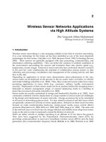
Fig. 7. Above part: The IEEE 802.15.4 Non Beacon-Enabled mode. Belo w part: The IEEE
802.15.4 Beacon-Enabled mode.
Emerging Communications for Wireless Sensor Networks134
0 10 20 30 40 50
0
0.1
0.2
0.3
0.4
0.5
0.6
0.7
0.8
0.9

1
P
MAC
(n)
N
GTS
=0, T
q
=15.36 [ms]
N
GTS
=0, T
q
=30.72 [ms]
N
GTS
=0, T
q
=61.44 [ms]
N
GTS
=4, T
q
=15.36 [ms]
N
GTS
=7, T
q
=30.72 [ms]
N

GTS
=7, T
q
=61.44 [ms]
(a)
0 10 20 30 40 50
n
0
0.1
0.2
0.3
0.4
0.5
0.6
0.7
0.8
0.9
1
P
MAC
(n)
D=2, T
q
=15.36 [ms]
D=2, T
q
=30.72 [ms]
D=2, T
q
=61.44 [ms]

D=10, T
q
=15.36 [ms]
D=10, T
q
=30.72 [ms]
D=10, T
q
=61.44 [ms]
(b)
Fig. 8. (a): P
MAC
(n) as a function of n, in the Beacon-Enabled case, for different values of SO
and N
GTS
, having fixed D = 2. (b): P
MAC
(n) as a function of n, in the Non Beacon-Enabled
case, for different values of T
q
and D.
If we compare the above Figures, we notice that once the superframe duration is fixed, re-
sults are approximatively the same if no GTSs are allocated, whereas, there is a co nsiderable
increment of P
MAC
(n) in the Beacon-Enabled case when GTSs are allocated. Note that the
cases T
q
= 15.36 [ms], T
q

= 30.72 [ms] and T
q
= 61.44 [ms] correspond to SO = 0, 1 and 2,
respectively.
7. Evaluation of the Area Throughput
The area throughput is mathematically derived through an intermediate step: firs t the prob-
ability of successful data transmission by an arbitrary sensor node, when k nodes are present
in the monitored area, is considered. Then, the overall area throughput is evaluated based on
this result.
7.1 Joint MAC/Connectivity Probability of Success
Let us consider an arbitrary sensor node that is located in the obse rved area A at a certain
time instant. T he aim is computing the probability that it can connect to one of the sinks
deployed in A and successfully transmit its data sample to the infrastructure. Such an e vent
is clearly related to connectivity issues (i.e., the se nsor must employ an adequate transmitting
power in order to reach the sink and not be isol ated) and to MAC problems (i.e., the number
of sensors which attempt at connecting to the same sink strongly affects the probability of
successful transmission). For this reason, we define P
s|k
(x, y) as the probability of successful
transmission conditioned on the overall number, k, of sensor s present in the mo nitored area,
which also depends on the position
(x, y) of the sensor relative to a reference system with
origin centered i n A. This dependence is due to the well-known border effects in connectivity
Bettstetter (2002).
In particular,
P
s|k
(x, y) = E
n
[P

MAC
(n) ·P
CON
(x, y)]
=
E
n
[P
MAC
(n)] · P
CON
(x, y). (36)
where the imp act of connectivity and MAC on the transmission of samples are separated. A
packet will be successfully received by a si nk if the sensor node is connected to at least one
sink and if no MAC failures occur. T he two terms that appear in (36) are now analysed.
P
CON
(x, y) represents the probability that the sensor is not isolated (i.e., it receives a suffi-
ciently strong s ignal from at least one sink). This probability decreases as the sensor ap-
proaches the borders (border effects). P
CON
for multi-sink single-hop WSNs, in bounded and
unbounded regions, has been computed in the previous Sections. In particular, for unbounded
regions, P
CON
(x, y)  P
CON
, that is equal to q
∞
, given by eq. (12). Whereas, when bounded

regions are considered, P
CON
(x, y) is equal to q(x, y) given by eq. (17).
Specifically, since the position of the sensor is in general unknown, P
s|k
(x, y) of (36) can be
deconditioned as follows:
P
s|k
= E
x,y
[P
s|k
(x, y)]
=
E
x,y
[P
CON
(x, y)] · E
n
[P
MAC
(n)] . (37)
E
x,y
[P
CON
(x, y)] is equal to q given by, e.g., eq. (25) when a rectangular region is accounted
for. When, instead border effects are negligible, E

x,y
[P
CON
(x, y)] = E
x,y
[P
CON
] = P
CON
, given
by eq. (12).
Given the channel model described in (2) (and following), the average connectivity area of the
sensor, that is the average area in which the sinks audible to the given sensor are contained,
can be defined as
A
σ
s
= πe
2(L
th
−k
0
)
k1
e
2σ
2
s
k
2

1
. (38)
In Fabbri & Verdone (2008) it is also shown that border effects are negligible when A
σ
s
< 0.1A.
In the following o nly this case will be accounted for. Thus we have
P
CON
(x, y)  P
CON
= 1 −e
−µ
0
, (39)
where µ
0
= ρ
0
A
σ
s
= I A
σ
s
/A is the mean number of audible sinks on an infinite plane from
any position Orriss & Barton (2003), being I
= ρ
0
· A the average number of sinks in A.

P
MAC
(n), n ≥ 1, is the probability of successful transmission when n −1 interfering sensors
are present introduced in Section 6 for the 802.15.4 MAC case.
Throughput Analysis of Wireless Sensor Networks via
Evaluation of Connectivity and MAC performance 135
0 10 20 30 40 50
0
0.1
0.2
0.3
0.4
0.5
0.6
0.7
0.8
0.9
1
P
MAC
(n)
N
GTS
=0, T
q
=15.36 [ms]
N
GTS
=0, T
q

=30.72 [ms]
N
GTS
=0, T
q
=61.44 [ms]
N
GTS
=4, T
q
=15.36 [ms]
N
GTS
=7, T
q
=30.72 [ms]
N
GTS
=7, T
q
=61.44 [ms]
(a)
0 10 20 30 40 50
n
0
0.1
0.2
0.3
0.4
0.5

0.6
0.7
0.8
0.9
1
P
MAC
(n)
D=2, T
q
=15.36 [ms]
D=2, T
q
=30.72 [ms]
D=2, T
q
=61.44 [ms]
D=10, T
q
=15.36 [ms]
D=10, T
q
=30.72 [ms]
D=10, T
q
=61.44 [ms]
(b)
Fig. 8. (a): P
MAC
(n) as a function of n, in the Beacon-Enabled case, for different values of SO

and N
GTS
, having fixed D = 2. (b): P
MAC
(n) as a function of n, in the Non Beacon-Enabled
case, for different values of T
q
and D.
If we compare the above Figures, we notice that once the superframe duration is fixed, re-
sults are approximatively the same if no GTSs are allocated, whereas, there is a co nsiderable
increment of P
MAC
(n) in the Beacon-Enabled case when GTSs are allocated. Note that the
cases T
q
= 15.36 [ms], T
q
= 30.72 [ms] and T
q
= 61.44 [ms] correspond to SO = 0, 1 and 2,
respectively.
7. Evaluation of the Area Throughput
The area throughput is mathematically derived through an intermediate step: firs t the prob-
ability of successful data transmission by an arbitrary sensor node, when k nodes are present
in the monitored area, is considered. Then, the overall area throughput is evaluated based on
this result.
7.1 Joint MAC/Connectivity Probability of Success
Let us consider an arbitrary sensor node that is located in the obse rved area A at a certain
time instant. T he aim is computing the probability that it can connect to one of the sinks
deployed in A and successfully transmit its data sample to the infrastructure. Such an e vent

is clearly related to connectivity issues (i.e., the sensor must employ an adequate transmitting
power in order to reach the sink and not be isol ated) and to MAC problems (i.e., the number
of sensors which attempt at connecting to the same sink strongly affects the probability of
successful transmission). For this reason, we define P
s|k
(x, y) as the probability of successful
transmission conditioned on the overall number, k, of sensor s present in the mo nitored area,
which also depends on the position
(x, y) of the sensor relative to a reference system with
origin centered i n A. This dependence is due to the well-known border effects in connectivity
Bettstetter (2002).
In particular,
P
s|k
(x, y) = E
n
[P
MAC
(n) ·P
CON
(x, y)]
=
E
n
[P
MAC
(n)] · P
CON
(x, y). (36)
where the imp act of connectivity and MAC on the transmission of samples are separated. A

packet will be successfully received by a si nk if the sensor node is connected to at least one
sink and if no MAC failures occur. T he two terms that appear in (36) are now analysed.
P
CON
(x, y) represents the probability that the sensor is not isolated (i.e., it receives a suffi-
ciently strong s ignal from at least one sink). This probability decreases as the sensor ap-
proaches the borders (border effects). P
CON
for multi-sink single-hop WSNs, in bounded and
unbounded regions, has been computed in the previous Sections. In particular, for unbounded
regions, P
CON
(x, y)  P
CON
, that is equal to q
∞
, given by eq. (12). Whereas, when bounded
regions are considered, P
CON
(x, y) is equal to q(x, y) given by eq. (17).
Specifically, since the position of the sensor is in general unknown, P
s|k
(x, y) of (36) can be
deconditioned as follows:
P
s|k
= E
x,y
[P
s|k

(x, y)]
=
E
x,y
[P
CON
(x, y)] · E
n
[P
MAC
(n)] . (37)
E
x,y
[P
CON
(x, y)] is equal to
q given by, e.g., eq. (25) when a rectangular region is accounted
for. When, instead border effects are negligible, E
x,y
[P
CON
(x, y)] = E
x,y
[P
CON
] = P
CON
, given
by eq. (12).
Given the channel model described in (2) (and following), the average connectivity area of the

sensor, that is the average area in which the sinks audible to the given sensor are contained,
can be defined as
A
σ
s
= πe
2(L
th
−k
0
)
k1
e
2σ
2
s
k
2
1
. (38)
In Fabbri & Verdone (2008) it is also shown that border effects are negligible when A
σ
s
< 0.1A.
In the following o nly this case will be accounted for. Thus we have
P
CON
(x, y)  P
CON
= 1 −e

−µ
0
, (39)
where µ
0
= ρ
0
A
σ
s
= I A
σ
s
/A is the mean number of audible sinks on an infinite plane from
any position Orriss & Barton (2003), being I
= ρ
0
· A the average number of sinks in A.
P
MAC
(n), n ≥ 1, is the probability of successful transmission when n −1 interfering sensors
are present introduced in Section 6 for the 802.15.4 MAC case.
Emerging Communications for Wireless Sensor Networks136
In general, when CSMA-based MAC protocols are considered, P
MAC
(n) is a monotonic de-
creasing function of the number, n, of sensors which attempt to connect to the same serving
sink. This number is in general a random variable in the range
[0, k]. In fact, note that in (36)
there is no explicit dependence on k, except for the fact that n

≤ k must hold. Moreover in our
case we assume 1
≤ n ≤ k, as there is at least one sensor competing for access with probability
P
CON
(39).
Orriss et al. (2002) showed that the number of sensors uniformly distributed on an infinite
plane that hear one particular sink as the one with the strongest signal power (i.e., the number
of sensors competing for access to such s ink), is Po isson distributed with mean
¯
n
= µ
s
1 − e
−µ
0
µ
0
, (40)
with µ
s
= ρ
s
A
σ
s
being the mean number of sensors that are audible by a given sink. Such a
result is relevant toward our goal even though it was der ived on the infinite plane. In fact,
when border effects are negligible (i.e., A
σ

s
< 0.1A) and k is large, n can still be considered
Poisson distributed. The only two things that change are:
• n is upper bounded by k (i.e., the pdf is truncated)
• the density ρ
s
is to be computed as the ratio k/A [m
−2
], thus yielding µ
s
= k
A
σ
s
A
.
Therefore, we assume n
∼ Poisson(
¯
n
), with
¯
n
=
¯
n
(k) = k
A
σ
s

A
1
−e
−µ
sink
µ
sink
= k
1
−e
−I A
σ
s
/A
I
. (41)
Finally, by taking the average in (37) explicit and neglecting border effects (see (39)), we get
P
s|k
= (1 −e
−I A
σ
s
/A
) ·
1
M
k
∑
n=1

P
MAC
(n)
¯
n
n
e
−
¯
n
n!
, (42)
where
M
=
k
∑
n=1
¯
n
n
e
−
¯
n
n!
(43)
is a normalizing factor.
7.2 Area Throughput
The amount of samples generated by the network as response to a g iven query is equal to

the number of sensors, k, that are present and active when the query is received. As a conse-
quence, the average number of data samples-per-query generated by the network is the mean
number of sensors,
¯
k, in the observed area.
Now denote by G the available area throughput, that is the average number of samples gen-
erated per unit of time, given by
G
=
¯
k
· f
q
= ρ
s
· A ·
1
T
q
[samples/sec]. (44)
From (44) we have
¯
k
= GT
q
.
The average amount of samples received by the infrastructure per unit of time (area through-
put), S, is given by:
S
=

+∞
∑
k=0
S(k) ·g
k
[samples/sec], (45)
where
S
(k) =
k
T
q
P
s|k
, (46)
g
k
as in (1) and P
s|k
as in (42).
Finally, by means of (42), (43) and (44), equation (45) may be rewritten as
S
=
1 −e
−I A
σ
s
/A
T
q

·
+∞
∑
k=1
∑
k
n
=1
P
MAC
(n)
¯
n
n
e
−
¯
n
n!
∑
k
n
=1
¯
n
n
e
−
¯
n

n!
·
(
GT
q
)
k
e
−GT
q
(k −1)!
. (47)
7.3 Numerical Results
In this section the area throughput obtained with the two modalities Beacon- and Non Beacon-
Enabled, considering different values o f D, SO, N
GTS
, T
q
and different connectivity levels, is
shown.
0 2000 4000 6000 8000 10000 12000 14000 16000 18000
0
1000
2000
3000
4000
5000
6000
G [samples/sec]
S(G) [samples/sec]

SO=0
SO=1
SO=2
BE S0=0, N
GTS
=0
BE S0=0, N
GTS
=2
BE S0=1, N
GTS
=0
BE S0=1, N
GTS
=6
BE S0=2, N
GTS
=0
BE S0=2, N
GTS
=7
Non Be Tq=15.36 msec
Non Be Tq=30.72 msec
Non Be Tq=64.44 msec
T
q
= 64.44
T
q
= 15.36

T
q
= 30.72
Fig. 9. S as a function of G, for the Beacon- and Non Beacon-Enabled cases, by varying SO,
N
GTS
and T
q
, having fixed D = 10.
In Figure 9, S as a function of G, when varying SO, N
GTS
and T
q
for D = 10, is shown. The
input parameters that we entered give a connection probability P
CON
= 0.89. It can be noted
Throughput Analysis of Wireless Sensor Networks via
Evaluation of Connectivity and MAC performance 137
In general, when CSMA-based MAC protocols are considered, P
MAC
(n) is a monotonic de-
creasing function of the number, n, of sensors which attempt to connect to the same serving
sink. This number is in general a random variable in the range
[0, k]. In fact, note that in (36)
there is no explicit dependence on k, except for the fact that n
≤ k must hold. Moreover in our
case we assume 1
≤ n ≤ k, as there is at least one sensor competing for access with probability
P

CON
(39).
Orriss et al. (2002) showed that the number of sensors uniformly distributed on an infinite
plane that hear one particular sink as the one with the strongest signal power (i.e., the number
of sensors competing for access to such s ink), is Poisson distributed with mean
¯
n
= µ
s
1 − e
−µ
0
µ
0
, (40)
with µ
s
= ρ
s
A
σ
s
being the mean number of sensors that are audible by a given sink. Such a
result is relevant toward our goal even though it was der ived on the infinite plane. In fact,
when border effects are negligible (i.e., A
σ
s
< 0.1A) and k is large, n can still be considered
Poisson distributed. The only two things that change are:
• n is upper bounded by k (i.e., the pdf is truncated)

• the density ρ
s
is to be computed as the ratio k/A [m
−2
], thus yielding µ
s
= k
A
σ
s
A
.
Therefore, we assume n
∼ Poisson(
¯
n
), with
¯
n
=
¯
n
(k) = k
A
σ
s
A
1
−e
−µ

sink
µ
sink
= k
1
−e
−I A
σ
s
/A
I
. (41)
Finally, by taking the average in (37) explicit and neglecting border effects (see (39)), we get
P
s|k
= (1 −e
−I A
σ
s
/A
) ·
1
M
k
∑
n=1
P
MAC
(n)
¯

n
n
e
−
¯
n
n!
, (42)
where
M
=
k
∑
n=1
¯
n
n
e
−
¯
n
n!
(43)
is a normalizing factor.
7.2 Area Throughput
The amount of samples generated by the network as response to a g iven query is equal to
the number of sensors, k, that are present and active when the query is received. As a conse-
quence, the average number of data samples-per-query generated by the network is the mean
number of sensors,
¯

k, in the observed area.
Now denote by G the available area throughput, that is the average number of samples gen-
erated per unit of time, given by
G
=
¯
k
· f
q
= ρ
s
· A ·
1
T
q
[samples/sec]. (44)
From (44) we have
¯
k
= GT
q
.
The average amount of samples received by the infrastructure per unit of time (area through-
put), S, is given by:
S
=
+∞
∑
k=0
S(k) ·g

k
[samples/sec], (45)
where
S
(k) =
k
T
q
P
s|k
, (46)
g
k
as in (1) and P
s|k
as in (42).
Finally, by means of (42), (43) and (44), equation (45) may be rewritten as
S
=
1 −e
−I A
σ
s
/A
T
q
·
+∞
∑
k=1

∑
k
n
=1
P
MAC
(n)
¯
n
n
e
−
¯
n
n!
∑
k
n
=1
¯
n
n
e
−
¯
n
n!
·
(
GT

q
)
k
e
−GT
q
(k −1)!
. (47)
7.3 Numerical Results
In this section the area throughput obtained with the two modalities Beacon- and Non Beacon-
Enabled, considering different values o f D, SO, N
GTS
, T
q
and different connectivity levels, is
shown.
0 2000 4000 6000 8000 10000 12000 14000 16000 18000
0
1000
2000
3000
4000
5000
6000
G [samples/sec]
S(G) [samples/sec]
SO=0
SO=1
SO=2
BE S0=0, N

GTS
=0
BE S0=0, N
GTS
=2
BE S0=1, N
GTS
=0
BE S0=1, N
GTS
=6
BE S0=2, N
GTS
=0
BE S0=2, N
GTS
=7
Non Be Tq=15.36 msec
Non Be Tq=30.72 msec
Non Be Tq=64.44 msec
T
q
= 64.44
T
q
= 15.36
T
q
= 30.72
Fig. 9. S as a function of G, for the Beacon- and Non Beacon-Enabled cases, by varying SO,

N
GTS
and T
q
, having fixed D = 10.
In Figure 9, S as a function of G, when varying SO, N
GTS
and T
q
for D = 10, is shown. The
input parameters that we entered give a connection probability P
CON
= 0.89. It can be noted
Emerging Communications for Wireless Sensor Networks138
that, once SO is fixed (Beacon-Enabled case), an increase of N
GTS
results in an increment of
S, since P
MAC
increases. Moreover, once N
GTS
is fixed, there exists a value of S O maximising
S. We can note that, a part for the case, Beacon-Enabled with GTSs allocated, an increase of
SO results in a decrement of S. In fact, even though P
MAC
gets greater the query interval
increases and the number of samples per second received by the s ink decreases. On the other
hand, when the Beacon-Enabled mode is used and GTSs are allocated, the optimum value of
SO is 1. This is due to the fact that, having large packets, when SO
= 0 too many packets are

lost, owing to the short duration of the superframe.
Concerning the Non Beacon-Enabled case, in both Figures it can be noted that, by decreasing
T
q
, S gets larger even though P
MAC
decreases, s ince, once again, the MAC losses are balanced
by larger values of f
q
.
0 0.2 0.4 0.6 0.8 1 1.2 1.4 1.6 1.8 2
x 10
4
0
500
1000
1500
2000
2500
3000
3500
4000
4500
5000
G [samples/sec]
S(G) [samples/sec]
D=2, Tq=128T
D=10, Tq=136T
Pcon=0.89
Pcon=1

Pcon=0.15
Fig. 10. S as a function of G, in the non beacon-enabled case, for different values of D and
P
CON
, having fixed T
q
to the maximum delay.
Finally, we show the effects of connectivity on the area throughput. When P
CON
is less than
1, only a fraction of the deploy ed nodes has a sink in its vicinity. In particular, an average
number,
¯
k
= P
CON
GT
q
/I, of sensors compete for access at each sink. In Figure 10 we consider
the non beacon-enabled case with D
= 2, T
q
= 128 T and D = 10, T
q
= 136 T. When D = 10,
T
q
= 136 T, for high G the area throughput tends to decay, since packet collisions d ominate.
Hence, by moving from P
CON

= 1 to P
CON
= 0.89, we observe a slight improvement due to
the fact that a smaller average number of sensors tries to connect to the same sink. Conversely,
when D
= 2, T
q
= 128 T, S is still increasing with G, then by moving from P
CON
= 1 to
P
CON
= 0.89, we just reduce the useful traffic. Furthermore, when P
CON
= 0.15, the available
area throughput is very light, so that we are working in the region where P
MAC
(D = 2, T
q
=
128T) < P
MAC
(D = 10, T
q
= 136 T), resulting in a slightly better performance of the case with
D
= 2. Thus we conclude that the effect of lowering P
CON
results in a stretch of the curves
reported in the previous plots.

8. Acknowledgments
This work was supported by the European Commission in the framework of the FP7 Network
of Excellence in Wireless Communications NEWCOM++ (contract n. 216715). Authors would
like to thank Roberto Verdone for the fruitful discussions about the model.
9. List of acronyms
r.v. random variable
PAN Personal Area Network
CAP Contention Access Period
CFP Contention Free Period
CSMA carrier-sense multiple access
CSMA/CA carrier-sense multiple access with collision avoidance
GTS Guaranteed Time Slot
ISM industrial scientific medical
MAC medium access control
p.d.f. probability distribution function
PPP Poisson Point Process
PAN pe rsonal area network
WSN wireless sensor network
10. References
Bettstetter, C. (2002). On the minimum node degree and connectivity of a wireless multihop
network, Mobile Ad Hoc Networks and Comp.(Mobihoc), Proc. ACM Symp. on.
Bettstetter, C. & Zangl, J. (2002). How to achieve a connected ad hoc network with ho-
mogeneous range assignment: an analytical study with consideration of border ef-
fects, Mobile and Wireless Commun ications Network, 2002 4th International Workshop on,
pp. 125–129.
Bianchi, G. (2000). Performance analysis of the ieee 802.11 distributed coordination function,
IEEE Journal on Selected Areas of Communication (JSAC) 18: 535–547.
Bollobàs, B. (2001). R andom Graphs, Cambridge University Press, second ed.
Buratti, C. (2009). A mathematical model for performance of ieee 802.15.4 beacon-enabled
mode, ACM IWCMC 2009, Leipzig, Germany, June 21-24.

Buratti, C. (2010). Performance analysis of ieee 802.15.4 beacon-enabled mode., Accepted for
publication on IEEE Transactions on Vehicular Technology.
Buratti, C. & Verdone, R. (2006). On the number of cluster heads minimizing the error rate
for a wireless sensor network using a hierarchical topology over ieee 802.15.4, Proc. of
IEEE Int. Symp. on Personal, Indoor and MoRadio Communications, PIMRC 2006, pp. 1–6.
Buratti, C. & Verdone, R. (2008). A mathematical model for per formance analysis of ieee
802.15.4 non-beacon enabled mode, Proc. IEEE European Wireless, EW2008, Prague,
Czech Republic.
Buratti, C. & Verdone, R. (2009). Performance analysis of ieee 802.15.4 non-beacon enabled
mode.
Throughput Analysis of Wireless Sensor Networks via
Evaluation of Connectivity and MAC performance 139
that, once SO is fixed (Beacon-Enabled case), an increase of N
GTS
results in an increment of
S, since P
MAC
increases. Moreover, once N
GTS
is fixed, there exists a value of S O maximising
S. We can note that, a part for the case, Beacon-Enabled with GTSs allocated, an increase of
SO results in a decrement of S. In fact, even though P
MAC
gets greater the query interval
increases and the number of samples per second received by the s ink decreases. On the other
hand, when the Beacon-Enabled mode is used and GTSs are allocated, the optimum value of
SO is 1. This is due to the fact that, having large packets, when SO
= 0 too many packets are
lost, owing to the short duration of the superframe.
Concerning the Non Beacon-Enabled case, in both Figures it can be noted that, by decreasing

T
q
, S gets larger even though P
MAC
decreases, s ince, once again, the MAC losses are balanced
by larger values of f
q
.
0 0.2 0.4 0.6 0.8 1 1.2 1.4 1.6 1.8 2
x 10
4
0
500
1000
1500
2000
2500
3000
3500
4000
4500
5000
G [samples/sec]
S(G) [samples/sec]
D=2, Tq=128T
D=10, Tq=136T
Pcon=0.89
Pcon=1
Pcon=0.15
Fig. 10. S as a function of G, in the non beacon-enabled case, for different values of D and

P
CON
, having fixed T
q
to the maximum delay.
Finally, we show the effects of connectivity on the area throughput. When P
CON
is less than
1, only a fraction of the deploy ed nodes has a sink in its vicinity. In particular, an average
number,
¯
k
= P
CON
GT
q
/I, of sensors compete for access at each sink. In Figure 10 we consider
the non beacon-enabled case with D
= 2, T
q
= 128 T and D = 10, T
q
= 136 T. When D = 10,
T
q
= 136 T, for high G the area throughput tends to decay, since packet collisions d ominate.
Hence, by moving from P
CON
= 1 to P
CON

= 0.89, we observe a slight improvement due to
the fact that a smaller average number of sensors tries to connect to the same sink. Conversely,
when D
= 2, T
q
= 128 T, S is still increasing with G, then by moving from P
CON
= 1 to
P
CON
= 0.89, we just reduce the useful traffic. Furthermore, when P
CON
= 0.15, the available
area throughput is very light, so that we are working in the region where P
MAC
(D = 2, T
q
=
128T) < P
MAC
(D = 10, T
q
= 136 T), resulting in a slightly better performance of the case with
D
= 2. Thus we conclude that the effect of lowering P
CON
results in a stretch of the curves
reported in the previous plots.
8. Acknowledgments
This work was supported by the European Commission in the framework of the FP7 Network

of Excellence in Wireless Communications NEWCOM++ (contract n. 216715). Authors would
like to thank Roberto Verdone for the fruitful discussions about the model.
9. List of acronyms
r.v. random variable
PAN Personal Area Network
CAP Contention Access Period
CFP Contention Free Period
CSMA carrier-sense multiple access
CSMA/CA carrier-sense multiple access with collision avoidance
GTS Guaranteed Time Slot
ISM industrial scientific medical
MAC medium access control
p.d.f. probability distribution function
PPP Poisson Point Process
PAN pe rsonal area network
WSN wireless sensor network
10. References
Bettstetter, C. (2002). On the minimum node degree and connectivity of a wireless multihop
network, Mobile Ad Hoc Networks and Comp.(Mobihoc), Proc. ACM Symp. on.
Bettstetter, C. & Zangl, J. (2002). How to achieve a connected ad hoc network with ho-
mogeneous range assignment: an analytical study with consideration of border ef-
fects, Mobile and Wireless Commun ications Network, 2002 4th International Workshop on,
pp. 125–129.
Bianchi, G. (2000). Perfor mance analysis of the i eee 802.11 distributed coordination function,
IEEE Journal on Selected Areas of Communication (JSAC) 18: 535–547.
Bollobàs, B. (2001). R andom Graphs, Cambridge University Press, second ed.
Buratti, C. (2009). A mathematical model for performance of ieee 802.15.4 beacon-enabled
mode, ACM IWCMC 2009, Leipzig, Germany, June 21-24.
Buratti, C. (2010). Performance analysis of ieee 802.15.4 beacon-enabled mode., Accepted for
publication on IEEE Transactions on Vehicular Technology.

Buratti, C. & Verdone, R. (2006). On the number of cluster heads minimizing the error rate
for a wireless sensor network using a hierarchical topology over ieee 802.15.4, Proc. of
IEEE Int. Symp. on Personal, Indoor and MoRadio Communications, PIMRC 2006, pp. 1–6.
Buratti, C. & Verdone, R. (2008). A mathematical model for per formance analysis of ieee
802.15.4 non-beacon enabled mode, Proc. IEEE European Wireless, EW2008, Prague,
Czech Republic.
Buratti, C. & Verdone, R. (2009). Performance analysis of ieee 802.15.4 non-beacon enabled
mode.
Emerging Communications for Wireless Sensor Networks140
Chen, Z., Lin, C., Wen, H. & Yin, H. (2007). An analytical model for evaluating ieee 802.15.4
csma/ca protocol in low rate wireless application, Proc. IEEE AINAW 2007.
Fabbri, F. & Verdone, R. (2008). Throughput analysis of an ieee 802.1lb multihop ad hoc net-
work, Proc. IEEE European Wireless, EW2008, Prague, Czech.
Gardner, W. (1989). Introduction to random processes: with applications to signals and systems,
second edn, McGraw Hi ll.
Kim, J. H. & Lee, J. K. (1999). Capture effects of wireless csma/ca protocols rayleigh and
shadow fading channels, IEEE Electronics Letters 48(4): 1277–1286.
Kim, T. O., Kim, H., Lee, J., Park, J. S. & Choi, B. D. (2006). Performance analysis of the ieee
802.15.4 with non beacon-enabled csma/ca in non-saturated contition, International
Conference on Embedded And Ubiquitous Computing, 2006. EUC 2006, pp. 884–893.
Meester, R. & Roy, R. (1996). Cambridge University Press, Cambridge UK.
Miorandi, D. & Altman, E. (2005). Coverage and connectivity of ad hoc networks in presence
of channel randomness, Proc. of 24th Annual Joint Con ference of the IEEE Computer and
Communications Societies, INFOCOM 2005., Vol. 1, pp. 491–502.
Misic, J., Misic, V. B. & Shafi, S. (2004). Performance of ieee 802.15.4 beacon-enabled pan with
uplink transmissions in non-saturation mode - access delay for finite buffers, Proc.
First I nternational Conference on Broadband Networks, 2004. BroadNets 2004, pp. 416–
425.
Misic, J., Shafi, S. & Misic, V. B. (2005). The impact of mac parameters on the performance of
802.15.4 pan, Elsevier Ad hoc Networks Journal 3: 509–528.

Misic, J., Shafi, S. & Misic, V. B. (2006). Maintaining reliability through activity management
in an 802.15.4 sensor cluster, 3: 779–788.
Orriss, J. & Barton, S. K. (2003). Probability distributions for the number of radio transceivers
which can communicate with one another, 51(4): 676–681.
Orriss, J., Phillips, A. & Barton, S. (1999). A statistical model for the spatial distribution of
mobiles and base stations, Proc. of IEEE Vehicular Technol. Conference, VTC 1999, Vol . 1,
pp. 19–22.
Orriss, J., Zanella, A., Verdone, R. & Barton, S. (2002). Probability distributions for the number
of radio tr ansceivers in a hot spot with an application to the evaluation of blocking
probabilities, IEEE Proc. of Personal, Indoor and Mobile Radio Communications, 2002,
Vol. 2.
Park, T., Kim, T., Choi, J., Choi, S. & Kwon, W. (2005). Throughput and energy consumption
analysis of ieee 802.15.4 slotted csma/ca, IEEE Electronics Letters 41: 1017–1019.
Penrose, M. D. (1993). On the spread-out limit for bond and continuum percolation, Annals of
Applied Probability 3: 253–276.
Penrose, M. D. (1999). On k-connectivity for a geometric random graph, Random Structures
and Algorithms 15: 145–164.
Penrose, M. D. & Pistztora, A. (1996). Large deviations for di screte and continous percolation,
Advances in Applied Probability 28: 29–52.
Pishro-Nik, Chan, K. & Fekri, F. (2004). On connectivity properties of large-scale sensor net-
works, Sensor and Ad Hoc Communications and Networks, 2004. IEEE SECON04. First
Annual IEEE Communications Society Conference on, pp. 498–507.
Pollin, S., Ergen, M., Ergen, S., Bougard, B., der Pierre, L. V. , Catthoor, F., Moerman, I., Bahai,
A. & Varaiya, P. (2008). Performance analysis of slotted carrier sense ieee 802.15.4
medium access layer, 7: 3359–3371.
Salbaroli, E. & Zanella, A. (2006). A statistical model for the evaluation of the distribution
of the received power in ad hoc and wireless sensor networks, Sensor and Ad Hoc
Communications and Networks, SECON ’06, 3rd Annual IEEE Communications Society
on, Vol. 3, pp. 756–760.
Santi, P. & Blough, D. M. (2003). The critical transmitting range for connectivity in sparse

wireless ad hoc networks, 2(1): 25–39.
Siripongwutikorn, P. (2006). Throughput analysis of an ieee 802.1lb multihop ad hoc network,
Proc. IEEE TE NCON 2006, pp. 1–4.
Stoyan, D., Kendall, W. S. & Mecke, J. (1995). Stochastic Geometry and its Applications.
Stuedi, P., Chinellato, O. & Alonso, G. (2005). Connectivity in the presence o f shadowing in
802.11 ad hoc networks, Proc. IEEE WCNC, 2005.
Takagi, H. & Kleinrock, L. (1985). Throughput analysis for persistent csma systems, 33(7): 627–
638.
Verdone, R., Dardari, D., Mazzini, G. & Conti, A. (2008). Wireless sensor and actuator networks,
Elsevier.
Vincze, Z., Vida, R. & Vidacs, A. (2007). D eploying multiple sinks in multi-hop wireles s sensor
networks, Pervasive Services, IEEE International C onference on, pp. 55–63.
Zdunek, K., Ucci, D. & Locicero, J. (1989). Throughput of nonpersistent inhibit s ense multiple
access with capture, IEEE Electronics Letters 25(1): 30–31.
Throughput Analysis of Wireless Sensor Networks via
Evaluation of Connectivity and MAC performance 141
Chen, Z., Lin, C., Wen, H. & Yin, H. (2007). An analytical model for evaluating ieee 802.15.4
csma/ca protocol in low rate wireless application, Proc. IEEE AINAW 2007.
Fabbri, F. & Verdone, R. (2008). Throughput analysis of an ieee 802.1lb multihop ad hoc net-
work, Proc. IEEE European Wireless, EW2008, Prague, Czech.
Gardner, W. (1989). Introduction to random processes: with applications to signals and systems,
second edn, McGraw Hi ll.
Kim, J. H. & Lee, J. K. (1999). Capture effects of wireless csma/ca protocols rayleigh and
shadow fading channels, IEEE Electronics Letters 48(4): 1277–1286.
Kim, T. O., Kim, H., Lee, J., Park, J. S. & Choi, B. D. (2006). Performance analysis of the ieee
802.15.4 with non beacon-enabled csma/ca in non-saturated contition, International
Conference on Embedded And Ubiquitous Computing, 2006. EUC 2006, pp. 884–893.
Meester, R. & Roy, R. (1996). Cambridge University Press, Cambridge UK.
Miorandi, D. & Altman, E. (2005). Coverage and connectivity of ad hoc networks in presence
of channel randomness, Proc. of 24th Annual Joint Con ference of the IEEE Computer and

Communications Societies, INFOCOM 2005., Vol. 1, pp. 491–502.
Misic, J., Misic, V. B. & Shafi, S. (2004). Performance of ieee 802.15.4 beacon-enabled pan with
uplink transmissions in non-saturation mode - access delay for finite buffers, Proc.
First I nternational Conference on Broadband Networks, 2004. BroadNets 2004, pp. 416–
425.
Misic, J., Shafi, S. & Misic, V. B. (2005). The impact of mac parameters on the performance of
802.15.4 pan, Elsevier Ad hoc Networks Journal 3: 509–528.
Misic, J., Shafi, S. & Misic, V. B. (2006). Maintaining reliability through activity management
in an 802.15.4 sensor cluster, 3: 779–788.
Orriss, J. & Barton, S. K. (2003). Probability distributions for the number of radio transceivers
which can communicate with one another, 51(4): 676–681.
Orriss, J., Phillips, A. & Barton, S. (1999). A statistical model for the spatial distribution of
mobiles and base stations, Proc. of IEEE Vehicular Technol. Conference, VTC 1999, Vol . 1,
pp. 19–22.
Orriss, J., Zanella, A., Verdone, R. & Barton, S. (2002). Probability distributions for the number
of radio transceivers in a hot spot with an application to the evaluation of blocking
probabilities, IEEE Proc. of Personal, Indoor and Mobi le Radio Communications, 2002,
Vol. 2.
Park, T., Kim, T., Choi, J., Choi, S. & Kwon, W. (2005). Throughput and energy consumption
analysis of ieee 802.15.4 slotted csma/ca, IEEE Electronics Letters 41: 1017–1019.
Penrose, M. D. (1993). On the spread-out limit for bond and continuum percolation, Annals of
Applied Probability 3: 253–276.
Penrose, M. D. (1999). On k-connectivity for a geometric random graph, Random Structures
and Algorithms 15: 145–164.
Penrose, M. D. & Pistztora, A. (1996). Large deviations for di screte and continous percolation,
Advances in Applied Probability 28: 29–52.
Pishro-Nik, Chan, K. & Fekri, F. (2004). On connectivity properties of large-scale sensor net-
works, Sensor and Ad Hoc Communications and Networks, 2004. IEEE SECON04. First
Annual IEEE Communications Society Conference on, pp. 498–507.
Pollin, S., Ergen, M., Ergen, S., Bougard, B., der Pierre, L. V. , Catthoor, F., Moerman, I., Bahai,

A. & Varaiya, P. (2008). Performance analysis of slotted carrier sense ieee 802.15.4
medium access layer, 7: 3359–3371.
Salbaroli, E. & Zanella, A. (2006). A statistical model for the evaluation of the distribution
of the received power in ad hoc and wireless sensor networks, Sensor and Ad Hoc
Communications and Networks, SECON ’06, 3rd Annual IEEE Communications Society
on, Vol. 3, pp. 756–760.
Santi, P. & Blough, D. M. (2003). The critical transmitting range for connectivity in sparse
wireless ad hoc networks, 2(1): 25–39.
Siripongwutikorn, P. (2006). Throughput analysis of an ieee 802.1lb multihop ad hoc network,
Proc. IEEE TENCON 2006, pp. 1–4.
Stoyan, D., Kendall, W. S. & Mecke, J. ( 1995). Stochastic Geometry and its Applications.
Stuedi, P., Chinellato, O. & Alonso, G. (2005). Connectivity in the presence o f shadowing in
802.11 ad hoc networks, Proc. IEEE WC NC, 2005.
Takagi, H. & Kleinrock, L. (1985). Throughput analysis for persistent csma systems, 33(7): 627–
638.
Verdone, R., Dardari, D., Mazzini, G. & Conti, A. (2008). Wireless sensor and actuator networks,
Elsevier.
Vincze, Z., Vida, R. & Vidacs, A. (2007). Deploying multiple sinks in multi-hop wireless sensor
networks, Pervasive Services, IEEE International C onference on, pp. 55–63.
Zdunek, K., Ucci, D. & Locicero, J. (1989). Throughput of nonpersistent inhibit sense multiple
access with capture, IEEE Electronics Letters 25(1): 30–31.
Emerging Communications for Wireless Sensor Networks142
Energy-aware Selective Communications in Sensor Networks 143
Energy-aware Selective Communications in Sensor Networks
Rocio Arroyo-Valles, Antonio G. Marques, Jesus Cid-Sueiro
0
Energy-aware Selective
Communications in Sensor Networks
Rocio Arroyo-Valles
(1)

, Antonio G. Marques
(2)
, Jesus Cid-Sueiro
(1)
(1)
Univ ersidad Carlos I I I de Madrid,
(2)
Univ ersidad Rey Juan Carlos de Madrid
Madrid, Spain
1. Introduction
During the last years, Wireless Sensor Networks (WSN) have attracted the attention of re-
searchers from electronics, signal processing, communications, and networking communities
due to their potential for providing new capabilities. Among the many design challenges that
have been identified, the ability of sensors to behave in an autonomous and self-organized
manner using limited energy and computation resources has emerged as a fundamental fac-
tor to take into account when WSN are deployed. In fact, the limitation of resources at the
network nodes is often a critical factor that conditions the design of applications for sensor
networks. Among the multiple limitations to consider, energy consumption emerges as a pri-
mary concern. This is because in many practical scenarios, sensor node batteries cannot be
(easily) refilled, thus nodes have a finite lifetime. Since every task carried out by the WSN has
an impact in terms of energy consumption, an enormous variety of solutions, both software
and hardware, have been proposed in the literature to optimize energy management; see, e.g.,
(Shih et al., 2001; Akyildiz et al., 2002).
Communication processes are typically among the most energy-expensive of such tasks.
Many works have focused on the minimization of the energy cost taking into account the
physical behavior of the WSN; see, e.g., (Shih et al., 2001; Marques et al., 2008; Wang et al.,
2008). However, energy savings can also be obtained by taking a higher level approach and
considering the different nature of the information that nodes have to transmit. This way, in
order to enlarge the network lifetime and optimize the overall network performance, sensor
nodes should weigh up: (a) the potential benefits of transmitting information and (b) the cost

of the subsequent communication process. A first step to address such optimum design is
to properly quantify or estimate both costs and benefits. This is possible in many practical
cases because the energy consumed during the different communications tasks (cost) is typ-
ically well-characterized and because applications where messages are graded according to
an importance indicator (benefit) are frequent in WSN. The message importance can be, for
instance, a priority value established by the routing protocol, or an information value spec-
ified by the application supported by the sensor network. Relevant examples in the context
of Sensor Networks can be found in the fields of: security (attack reports (Wood & Stankovic,
2002)), medical care (critical alerts (Shnayder et al., 2005)), or data fusion (DAIDA algorithm
in (Qiu et al., 2005)), to name a few.
In such scenarios, energy in WSN can be saved by making intelligent importance-driven de-
cisions about message transmission, in an autonomous and self-organized manner, adapting
8
Emerging Communications for Wireless Sensor Networks144
forwarding decisions to the traffic importance. This way, a selective forwarding scheme allows
nodes to keep the capacity for managing their own resources at the same time that optimizes
communication expenses by only transmitting the most relevant messages.
That is precisely the objective pursued in this work: to develop optimum selective message
forwarding schemes for energy-limited sensor networks where sensors (re-) transmit mes-
sages of different importance (priority). In order to decide whether to transmit or discard a
message, sensors will take into account factors such as the energy consumed during the dif-
ferent tasks that a sensor has to carry out (transmission, reception, etc.), the available battery,
the importance of the received message, the statistical model of such importances, or their
neighbors’ behavior.
Related ideas have recently been explored in literature. The IDEALS algorithm (Merrett et al.,
2005), built under the concept of message and power priorities, tries to extend network life-
time for important messages, discarding all messages except those of high importance when
battery resources are scarce. The PGR (Prioritized Geographical Routing) algorithm (Mujum-
dar, 2004) selects the appropriated routing technique depending on the priority of the message
(low, medium or high). Moreover, a fuzzy logic approach to deal with message transfer pri-

ority arbitration that considers fifteen different priority levels has been presented in (Rivera
et al., 2007). Rather than using a heuristic approach, the aim here is to obtain analytical re-
sults that building on a mathematical formulation, provide basic guidelines to design such
energy-efficient schemes. This will be done by following a probabilistic and statistical ap-
proach that will open the door to a long-term optimization of the network. The optimal for-
warding schemes will be obtained then as the optimal solution of the formulated problem.
1
The initial step will be to carefully select the model for the WSN. On the one hand the model
has to be rich enough so that different real scenarios can be fit into, on the other hand it
has to be simple enough so that the mathematical formulation is tractable and closed-form
solutions can be derived. This way, basic principles to guide the design of energy-efficient
importance-driven schemes can be identified. Once the mathematical model is set, we will
derive optimum schemes for three different scenarios.
First we will consider the case when the forwarding schemes are designed so that sensors max-
imize the importance of their own transmitted messages. Second, we enrich the model by also
considering the behavior of neighboring nodes. Third, we develop a forwarding scheme for
nodes optimizing the importance of the messages that successfully arrive to the sink. Clearly,
from an overall network efficiency perspective the first scenario will perform worse than its
counterparts, but it will require less signaling overhead. On the contrary, the last scheme
will optimize the overall network performance, but it will require full coordination among
the nodes of the WSN. Differences among the proposed schemes will be quantified both from
a theoretical and numerical perspective. Together with those optimal schemes, suboptimal
schemes that operate under less demanding conditions than those for the optimal ones are
also developed.
2
1
Noticeably, the statistical model presented in this chapter exhibits similarities to other problems in
Operations Research and Stochastic Dynamic Programming (see, e.g., (Sennott, 1999)), and the equations
describing the energy evolution at the sensor node and the importance sum can be restated as a par-
ticular type of Markov decision process. Nonetheless, our treatment of the problem and the theoretical

derivations are self-contained.
2
To facilitate exposition, most of the chapter will be devoted to the first (and simplest) scenario. Never-
theless it should be noted that the specific results presented only for that scenario can be easily extended
to the other two scenarios. Under the same philosophy, no mathematical proofs have been included in
the chapter. Readers who are interested can always check our original work in (Arroyo-Valles et al., 2009;
It will be shown that in most cases, the optimal forwarding scheme is fairly simple. More
specifically, it will turn out that the optimal decision is made comparing the importance of the
received message with a threshold whose optimum value varies along time. We will show
that our schemes improve the global performance in terms of quantity and quality of the
messages that really arrive at the destination node. Finally, it will be also shown that the gain
of the selective forwarding schemes (compared to a non-selective ones) will critically depend
on factors such as the relationship among the energy consumed during each of the tasks that
nodes have to implement, the frequency of idle times, or the statistical distribution of the
importances, to name a few.
The theoretical results will be complemented with numerical simulations that not only will
corroborate the theoretical claims but also will help us to quantify the gains of implementing
the selective scheme for a broader range of practical scenarios.
It is worth stressing that besides the theoretical value of this work: (i) the developed schemes
can eventually be incorporated into many existing routing protocols; and (ii) our approach
can also be easily integrated with a variety of existing data collection approaches, including
schemes that support in network data aggregation.
2. Sensor model
For the purpose of the analysis that follows, we consider a sensor network as a collection
of nodes
N = {n|n = 0,. . . , N − 1}. For the time being, we will focus on the behavior of each
node, which receives a sequence of requests to transmit messages (no matter how the network
topology is). The node dynamics will be characterized by two variables
• e
k

: available energy at a given node at time k. It reflects the “internal state” of the node;
and
• x
k
: importance of the message to be sent at time k. It reflects the “external input” to the
node.
For mathematical reasons, we assume that if the node does not receive any request to transmit
at time k, then x
k
= 0, while true messages will have x
k
> 0.
At time k, the sensor node must make a decision, d
k
, about sending or not the current message,
so that d
k
= 1 if the message is sent, and d
k
= 0 if the node decides to discard it.
Nodes consume energy at each time slot, by an amount that depends on the message reception
and the taken actions. In the literature, up to three different energy expenses are typically
considered:
• E
I
: energy spent at a silent time, when there is no message reception, and the node may
stay at ”idle” mode;
• E
R
: energy spent when receiving a message; and

• E
T
: energy spent when transmitting a message.
The value of these parameters will depend on the system specifications and the specific appli-
cation (among the factors that will determine the energy costs we find mobility, sensed mag-
nitude, or behavior of the batteries, to name a few). For example, for static dense networks, E
T
and E
R
values may be very similar, while for mobile networks operating over fading channels,
E
T
>> E
R
is expected.
2008).
Energy-aware Selective Communications in Sensor Networks 145
forwarding decisions to the traffic importance. This way, a selective forwarding scheme allows
nodes to keep the capacity for managing their own resources at the same time that optimizes
communication expenses by only transmitting the most relevant messages.
That is precisely the objective pursued in this work: to develop optimum selective message
forwarding schemes for energy-limited sensor networks where sensors (re-) transmit mes-
sages of different importance (priority). In order to decide whether to transmit or discard a
message, sensors will take into account factors such as the energy consumed during the dif-
ferent tasks that a sensor has to carry out (transmission, reception, etc.), the available battery,
the importance of the received message, the statistical model of such importances, or their
neighbors’ behavior.
Related ideas have recently been explored in literature. The IDEALS algorithm (Merrett et al.,
2005), built under the concept of message and power priorities, tries to extend network life-
time for important messages, discarding all messages except those of high importance when

battery resources are scarce. The PGR (Prioritized Geographical Routing) algorithm (Mujum-
dar, 2004) selects the appropriated routing technique depending on the priority of the message
(low, medium or high). Moreover, a fuzzy logic approach to deal with message transfer pri-
ority arbitration that considers fifteen different priority levels has been presented in (Rivera
et al., 2007). Rather than using a heuristic approach, the aim here is to obtain analytical re-
sults that building on a mathematical formulation, provide basic guidelines to design such
energy-efficient schemes. This will be done by following a probabilistic and statistical ap-
proach that will open the door to a long-term optimization of the network. The optimal for-
warding schemes will be obtained then as the optimal solution of the formulated problem.
1
The initial step will be to carefully select the model for the WSN. On the one hand the model
has to be rich enough so that different real scenarios can be fit into, on the other hand it
has to be simple enough so that the mathematical formulation is tractable and closed-form
solutions can be derived. This way, basic principles to guide the design of energy-efficient
importance-driven schemes can be identified. Once the mathematical model is set, we will
derive optimum schemes for three different scenarios.
First we will consider the case when the forwarding schemes are designed so that sensors max-
imize the importance of their own transmitted messages. Second, we enrich the model by also
considering the behavior of neighboring nodes. Third, we develop a forwarding scheme for
nodes optimizing the importance of the messages that successfully arrive to the sink. Clearly,
from an overall network efficiency perspective the first scenario will perform worse than its
counterparts, but it will require less signaling overhead. On the contrary, the last scheme
will optimize the overall network performance, but it will require full coordination among
the nodes of the WSN. Differences among the proposed schemes will be quantified both from
a theoretical and numerical perspective. Together with those optimal schemes, suboptimal
schemes that operate under less demanding conditions than those for the optimal ones are
also developed.
2
1
Noticeably, the statistical model presented in this chapter exhibits similarities to other problems in

Operations Research and Stochastic Dynamic Programming (see, e.g., (Sennott, 1999)), and the equations
describing the energy evolution at the sensor node and the importance sum can be restated as a par-
ticular type of Markov decision process. Nonetheless, our treatment of the problem and the theoretical
derivations are self-contained.
2
To facilitate exposition, most of the chapter will be devoted to the first (and simplest) scenario. Never-
theless it should be noted that the specific results presented only for that scenario can be easily extended
to the other two scenarios. Under the same philosophy, no mathematical proofs have been included in
the chapter. Readers who are interested can always check our original work in (Arroyo-Valles et al., 2009;
It will be shown that in most cases, the optimal forwarding scheme is fairly simple. More
specifically, it will turn out that the optimal decision is made comparing the importance of the
received message with a threshold whose optimum value varies along time. We will show
that our schemes improve the global performance in terms of quantity and quality of the
messages that really arrive at the destination node. Finally, it will be also shown that the gain
of the selective forwarding schemes (compared to a non-selective ones) will critically depend
on factors such as the relationship among the energy consumed during each of the tasks that
nodes have to implement, the frequency of idle times, or the statistical distribution of the
importances, to name a few.
The theoretical results will be complemented with numerical simulations that not only will
corroborate the theoretical claims but also will help us to quantify the gains of implementing
the selective scheme for a broader range of practical scenarios.
It is worth stressing that besides the theoretical value of this work: (i) the developed schemes
can eventually be incorporated into many existing routing protocols; and (ii) our approach
can also be easily integrated with a variety of existing data collection approaches, including
schemes that support in network data aggregation.
2. Sensor model
For the purpose of the analysis that follows, we consider a sensor network as a collection
of nodes
N = {n|n = 0,. . . , N − 1}. For the time being, we will focus on the behavior of each
node, which receives a sequence of requests to transmit messages (no matter how the network

topology is). The node dynamics will be characterized by two variables
• e
k
: available energy at a given node at time k. It reflects the “internal state” of the node;
and
• x
k
: importance of the message to be sent at time k. It reflects the “external input” to the
node.
For mathematical reasons, we assume that if the node does not receive any request to transmit
at time k, then x
k
= 0, while true messages will have x
k
> 0.
At time k, the sensor node must make a decision, d
k
, about sending or not the current message,
so that d
k
= 1 if the message is sent, and d
k
= 0 if the node decides to discard it.
Nodes consume energy at each time slot, by an amount that depends on the message reception
and the taken actions. In the literature, up to three different energy expenses are typically
considered:
• E
I
: energy spent at a silent time, when there is no message reception, and the node may
stay at ”idle” mode;

• E
R
: energy spent when receiving a message; and
• E
T
: energy spent when transmitting a message.
The value of these parameters will depend on the system specifications and the specific appli-
cation (among the factors that will determine the energy costs we find mobility, sensed mag-
nitude, or behavior of the batteries, to name a few). For example, for static dense networks, E
T
and E
R
values may be very similar, while for mobile networks operating over fading channels,
E
T
>> E
R
is expected.
2008).
Emerging Communications for Wireless Sensor Networks146
Energy at time k can be expressed recursively as
e
k+1
= e
k
− d
k
E
1
(x

k
) − (1 − d
k
)E
0
(x
k
), (1)
where E
1
(x
k
) is the energy consumed when the node decides to transmit the message, and
E
0
(x
k
) is the energy consumed when the message is discarded. For positive values of impor-
tance, energy consumption is independent of the message importance, and we have
E
1
(x
k
) = E
T
+ E
R
, x
k
> 0 (2)

E
0
(x
k
) = E
R
, x
k
> 0. (3)
Recalling that x
k
= 0 means that no messages are received, we also have
E
1
(0) = E
0
(0) = E
I
. (4)
When the sensor node is the source of the message, E
R
comprises the energy expense of the
message generation process (possibly by a sensing device). When the sensor node acts as a
forwarder, E
R
comprises the energy expense of receiving the message from other node. Thus,
we assume that E
R
is the same no matter if the node is the source of the message or it has been
requested to forward a message from other node. Even though this assumption is not critical

and could be bypassed by splitting E
R
between receiving and sensing costs, we adopt it for
two reasons: (i) it leads to a simpler mathematical formulation and (ii) nodes are prevented
from acting selfishly (note that if the energy cost of sensing were smaller than the cost of
receiving, nodes would promote their own messages instead of forwarding others’ messages).
Remark 1 It is important to mention that although this chapter focuses on the case where the energy
consumption is given by (2)-(4), we will formulate and solve the general case in (1) by assuming
that both consumption profiles, E
1
(x) and E
0
(x), may arbitrarily depend on x. As a first approach,
the model could even be applied to situations where E
T
and E
R
are random or time-variant (e.g., in
sensors operating over fast fading channels where transmissions are adapted based on the channel state
information) by substituting E
T
and E
R
by their respective mathematical expectations. In any case, we
assume that both energy functions are perfectly known.
3. Optimal selective transmission
To derive an optimal transmission policy we will consider that node decisions do not depend
on the state and the actions of neighboring nodes, but only on the available information at
each node. Therefore, at each time, k, the node decision depends on the internal state and the
external input

d
k
= g(e
k
, x
k
), (5)
with the constraint
g
(e
k
, x
k
) = 0, if e
k
< E
1
(x
k
) (6)
reflecting that, if the sensor node does not have enough energy to receive and transmit the
message, it cannot decide d
k
= 1.
Decisions at each node will be made with infinite horizon, i.e., by maximizing (on average) the
importance sum of all transmitted messages
s
∞
=
∞

∑
k=0
d
k
x
k
. (7)
Since nodes have limited energy resources, this sum only contains a finite number of nonzero
values (eventually, for some k, e
k
< min
k
E
1
(x
k
), and ∀k

≥ k, we have d
k

= 0).
The following result provides an optimal selective transmitter.
Theorem 1 Let
{x
k
,k ≥ 0} be a statistically independent sequence of importance values, and
e
k
the energy process driven by (1). Consider the sequence of decision rules

d
k
= u(x
k
− µ
k
(e
k
, x
k
))u(e
k
− E
1
(x
k
)), (8)
where u
(x) stands for the Heaviside step function (with the convention u(0) = 1), and µ
k
is
defined recursively through the pair of equations
µ
k
(e, x) = λ
k+1
(e − E
0
(x)) − λ
k+1

(e − E
1
(x)) (9)
λ
k
(e) =
(
E{λ
k+1
(e − E
0
(x
k
))} + E{(x
k
− µ
k
(e, x
k
))
+
u(e − E
1
(x
k
))}

u
(e), (10)
where

(z)
+
= zu( z), for any z.
The sequence
{d
k
} is optimal in the sense of maximizing E{s
∞
} (with s
∞
given by (7)), among
all sequences in the form d
k
= g(e
k
, x
k
) (with g(e
k
, x
k
) = 0 for e
k
< E
1
(x
k
)).
The auxiliary function λ
k

(e) represents the expected increment of the total importance (ex-
pected reward) at time k , i.e.,
λ
k
(e) =
∞
∑
i=k
E{d
i
x
i
|e
k
= e}. (11)
The proof can be found in (Arroyo-Valles et al., 2009). Although Theorem 1 holds for any
energy cost and importance value, it does not provide a clear intuition about the impact of
E
0
(x) and E
1
(x) and the distribution of x
k
on the design of the optimal transmission scheme.
Moreover, the direct application of this theorem is difficult, because (9) and (10) state a time-
reversed recursive relation: in order to make optimal decisions, the node should know the
future importance distributions in advance. For these reasons, in the reminder of this chapter
we will focus special attention on several particular cases that will lead us to tractable closed-
form solutions.
3.1 Stationarity

If all variables x
1
,. . . , x
k
have the same distribution, then µ
k
does not depend on k [c.f. (9) and
(10)]. In this case, the following result can be shown (see (Arroyo-Valles et al., 2009)):
Theorem 2 Under the conditions of Th. 1, if the importance values
{x
k
,k ≥ 0} are identically dis-
tributed and inf
x
{E
i
(x)} > 0, for i = 0, 1, the sequence of decision rules given by
d
k
= u(x
k
− µ(e
k
, x
k
))u(e − E
1
(x
k
)), (12)

where
µ
(e, x) = λ(e − E
0
(x)) − λ(e − E
1
(x)) (13)
λ
(e) =
(
E{λ(e − E
0
(x))} + E{(x − µ(e, x))
+
u(e − E
1
(x))}

u
(e), (14)
Energy-aware Selective Communications in Sensor Networks 147
Energy at time k can be expressed recursively as
e
k+1
= e
k
− d
k
E
1

(x
k
) − (1 − d
k
)E
0
(x
k
), (1)
where E
1
(x
k
) is the energy consumed when the node decides to transmit the message, and
E
0
(x
k
) is the energy consumed when the message is discarded. For positive values of impor-
tance, energy consumption is independent of the message importance, and we have
E
1
(x
k
) = E
T
+ E
R
, x
k

> 0 (2)
E
0
(x
k
) = E
R
, x
k
> 0. (3)
Recalling that x
k
= 0 means that no messages are received, we also have
E
1
(0) = E
0
(0) = E
I
. (4)
When the sensor node is the source of the message, E
R
comprises the energy expense of the
message generation process (possibly by a sensing device). When the sensor node acts as a
forwarder, E
R
comprises the energy expense of receiving the message from other node. Thus,
we assume that E
R
is the same no matter if the node is the source of the message or it has been

requested to forward a message from other node. Even though this assumption is not critical
and could be bypassed by splitting E
R
between receiving and sensing costs, we adopt it for
two reasons: (i) it leads to a simpler mathematical formulation and (ii) nodes are prevented
from acting selfishly (note that if the energy cost of sensing were smaller than the cost of
receiving, nodes would promote their own messages instead of forwarding others’ messages).
Remark 1 It is important to mention that although this chapter focuses on the case where the energy
consumption is given by (2)-(4), we will formulate and solve the general case in (1) by assuming
that both consumption profiles, E
1
(x) and E
0
(x), may arbitrarily depend on x. As a first approach,
the model could even be applied to situations where E
T
and E
R
are random or time-variant (e.g., in
sensors operating over fast fading channels where transmissions are adapted based on the channel state
information) by substituting E
T
and E
R
by their respective mathematical expectations. In any case, we
assume that both energy functions are perfectly known.
3. Optimal selective transmission
To derive an optimal transmission policy we will consider that node decisions do not depend
on the state and the actions of neighboring nodes, but only on the available information at
each node. Therefore, at each time, k, the node decision depends on the internal state and the

external input
d
k
= g(e
k
, x
k
), (5)
with the constraint
g
(e
k
, x
k
) = 0, if e
k
< E
1
(x
k
) (6)
reflecting that, if the sensor node does not have enough energy to receive and transmit the
message, it cannot decide d
k
= 1.
Decisions at each node will be made with infinite horizon, i.e., by maximizing (on average) the
importance sum of all transmitted messages
s
∞
=

∞
∑
k=0
d
k
x
k
. (7)
Since nodes have limited energy resources, this sum only contains a finite number of nonzero
values (eventually, for some k, e
k
< min
k
E
1
(x
k
), and ∀k

≥ k, we have d
k

= 0).
The following result provides an optimal selective transmitter.
Theorem 1 Let
{x
k
,k ≥ 0} be a statistically independent sequence of importance values, and
e
k

the energy process driven by (1). Consider the sequence of decision rules
d
k
= u(x
k
− µ
k
(e
k
, x
k
))u(e
k
− E
1
(x
k
)), (8)
where u
(x) stands for the Heaviside step function (with the convention u(0) = 1), and µ
k
is
defined recursively through the pair of equations
µ
k
(e, x) = λ
k+1
(e − E
0
(x)) − λ

k+1
(e − E
1
(x)) (9)
λ
k
(e) =
(
E{λ
k+1
(e − E
0
(x
k
))} + E{(x
k
− µ
k
(e, x
k
))
+
u(e − E
1
(x
k
))}

u
(e), (10)

where
(z)
+
= zu( z), for any z.
The sequence
{d
k
} is optimal in the sense of maximizing E{s
∞
} (with s
∞
given by (7)), among
all sequences in the form d
k
= g(e
k
, x
k
) (with g(e
k
, x
k
) = 0 for e
k
< E
1
(x
k
)).
The auxiliary function λ

k
(e) represents the expected increment of the total importance (ex-
pected reward) at time k , i.e.,
λ
k
(e) =
∞
∑
i=k
E{d
i
x
i
|e
k
= e}. (11)
The proof can be found in (Arroyo-Valles et al., 2009). Although Theorem 1 holds for any
energy cost and importance value, it does not provide a clear intuition about the impact of
E
0
(x) and E
1
(x) and the distribution of x
k
on the design of the optimal transmission scheme.
Moreover, the direct application of this theorem is difficult, because (9) and (10) state a time-
reversed recursive relation: in order to make optimal decisions, the node should know the
future importance distributions in advance. For these reasons, in the reminder of this chapter
we will focus special attention on several particular cases that will lead us to tractable closed-
form solutions.

3.1 Stationarity
If all variables x
1
,. . . , x
k
have the same distribution, then µ
k
does not depend on k [c.f. (9) and
(10)]. In this case, the following result can be shown (see (Arroyo-Valles et al., 2009)):
Theorem 2 Under the conditions of Th. 1, if the importance values
{x
k
,k ≥ 0} are identically dis-
tributed and inf
x
{E
i
(x)} > 0, for i = 0, 1, the sequence of decision rules given by
d
k
= u(x
k
− µ(e
k
, x
k
))u(e − E
1
(x
k

)), (12)
where
µ
(e, x) = λ(e − E
0
(x)) − λ(e − E
1
(x)) (13)
λ
(e) =
(
E{λ(e − E
0
(x))} + E{(x − µ(e, x))
+
u(e − E
1
(x))}

u
(e), (14)
Emerging Communications for Wireless Sensor Networks148
is optimal in the sense of maximizing E{s
∞
} among all sequences of decision rules in the form
d
k
= g(e
k
, x

k
) (with g(e
k
, x
k
) = 0 for e
k
< E
1
(x
k
)).
It is important to stress that in most scenarios involving multiple sensors, the stationarity as-
sumption, strictly speaking, is not true. For example, the distribution of messages arriving
to a node depends on the transmission policy used by forwarding nodes. Since the optimal
policy presented here is energy-dependent [c.f. either (9) or (13)] and the available energy
clearly changes along time for all nodes, the importance distribution of the received messages
will also change along time. However, it will be shown in the next sections that the simplifi-
cation obtained in (13) is not only useful from a theoretical perspective, but also valid from a
practical point of view for large networks. This (almost) stationary behavior can be justified
based on different reasons. First, although the optimal forwarding policy varies along time,
this variation turns out to be negligible during most of the time (i.e., it is almost-stationary).
The underlying reason is that for medium-high values of available energy the optimal for-
warding scheme is not very sensitive to energy changes. Only when nodes are close to run
out of batteries, the decision threshold varies significantly as a function of the remaining en-
ergy. Second, even if the behavior of a single node is not stationary, the aggregate effect of
the entire network may be stationary. In other words, the approximation given by (13) will
be accurate during most of the time, and the discrepancy will only arise when the network is
close to expire. Theoretical analysis and numerical results will corroborate this intuition.
3.2 Constant energy profiles

Under the constant profile model given by (2)-(4), the optimal threshold can be written as
µ
k
(e, x) = µ
k
(e)I
x>0
, (15)
where I
x>0
is an indicator function (equal to unity if the condition holds and zero otherwise),
and using (9) we have
µ
k
(e) = λ
k+1
(e − E
R
) − λ
k+1
(e − E
T
− E
R
). (16)
Also, (10) becomes
λ
k
(e) = P
I

λ
k+1
(e − E
I
) + (1 − P
I
)λ
k+1
(e − E
R
) − P
I
µ
k
(e,0)u(−µ
k
(e,0))u(e − E
I
)
+ (
1 − P
I
)E{(x
k
− µ
k
(e, x
k
))
+

|x
k
> 0} · u(e − E
T
− E
R
)
=
P
I
λ
k+1
(e − E
I
) + (1 − P
I
)λ
k+1
(e − E
R
)
+ (
1 − P
I
)E{(x
k
− µ
k
(e, x
k

))
+
|x
k
> 0} · u(e − E
T
− E
R
) (17)
where P
I
= Pr{x = 0}. Defining
H
k
(µ) = E{(x
k
− µ)
+
|x
k
> 0}, (18)
we can write
λ
k
(e) = P
I
λ
k+1
(e − E
I

) + (1 − P
I
)λ
k+1
(e − E
R
)
+(
1 − P
I
)H(µ
k
(e))u(e − E
T
− E
R
). (19)
Thus, the optimal transmission policy for a sensor with a constant energy profile is described
by (16) and (19). In order to analyze the influence of idle times and the relation between
transmission and reception energy expenses separately, in the following examples we consider
the case of P
I
= 0 and/or E
I
= 0. Note that if any of these conditions holds, the expected
importance sum in (19) can be rewritten as
λ
k
(e) = λ
k+1

(e − E
R
) + H( µ
k
(e))u(e − E
T
− E
R
). (20)
3.3 Examples
As we have already mentioned, there is no general explicit solution to the pair of equations
(9) and (10), not even for the stationary case in (16) and (19). For this reason, in this section
we focus on systems satisfying the operating conditions that gave rise to (20) (constant energy
profiles, stationarity and zero idle energy) and solve the recursive relations for several impor-
tance distributions
3
. This simplification will lead to tractable expressions, providing insight
into the behavior of the optimal forwarding scheme.
• Uniform Distribution: Let U
(0,2) denote the uniform distribution between 0 and 2
whose probability density function (PDF) is
p
(x) =
1
2
(u(x) − u(x − 2)). (21)
Substituting (21) into (18), we have
H
(µ) = E{(x − µ)
+

} =
1
4
(2 − µ)
2
, (22)
and therefore, the expected reward is given by
λ
(e) = λ(e − E
R
) +
1
4
(2 − µ(e))
2
u(e − E
T
− E
R
). (23)
Figure 1(a) plots the threshold for extremely small values of available energy, e. E
1
(x) = 1
and different values of the ratio E
T
/E
R
are considered. Note that, for values of e lower
than 1, in spite of the threshold value is 0, there is no actual transmission because u
(e −

E
T
− E
R
) = 0. For 1 < e < E
1
+ E
R
there is only one opportunity to send the message,
so the threshold is also 0, which means that the message will be transmitted whatever
its importance value is. For larger energy values, the threshold increases, meaning that
the transmission can be made more selective. Note, also, that µ
(e) evolves in a staircase
manner, because any energy amount in excess of a multiple of E
R
is useless.
Figure 1(b) represents the expected reward (λ
(e)). Note that the case E
T
= 0 is equiva-
lent to a non-selective transmitter (because, according to (16), the optimal threshold is
0 in that case, which means that no messages are discarded). Despite that, for e close
to 2, there is not energy for a second transmission, the selective transmitter provides a
significant expected income with respect to the non-selective one.
Figure 2(a) shows the optimal threshold for E
T
= 4, E
R
= 1 and high values of available
energy. Note the sawtooth shape of the forwarding threshold: as the available energy is

reduced to a value close to a multiple of the energy required to transmit, the forward-
ing threshold decreases, because if there is not any transmissions, the total number of
possible messages to be sent is reduced by a unity.
Figure 2(b) represents the expected reward of the selective transmitter (continuous line)
and the non-selective one (dotted line), which transmits all messages regardless of their
importance value, until energy is used up.
3
In the following, free parameters will be set so that all importance distributions have a mean value
equal to one.
Energy-aware Selective Communications in Sensor Networks 149
is optimal in the sense of maximizing E{s
∞
} among all sequences of decision rules in the form
d
k
= g(e
k
, x
k
) (with g(e
k
, x
k
) = 0 for e
k
< E
1
(x
k
)).

It is important to stress that in most scenarios involving multiple sensors, the stationarity as-
sumption, strictly speaking, is not true. For example, the distribution of messages arriving
to a node depends on the transmission policy used by forwarding nodes. Since the optimal
policy presented here is energy-dependent [c.f. either (9) or (13)] and the available energy
clearly changes along time for all nodes, the importance distribution of the received messages
will also change along time. However, it will be shown in the next sections that the simplifi-
cation obtained in (13) is not only useful from a theoretical perspective, but also valid from a
practical point of view for large networks. This (almost) stationary behavior can be justified
based on different reasons. First, although the optimal forwarding policy varies along time,
this variation turns out to be negligible during most of the time (i.e., it is almost-stationary).
The underlying reason is that for medium-high values of available energy the optimal for-
warding scheme is not very sensitive to energy changes. Only when nodes are close to run
out of batteries, the decision threshold varies significantly as a function of the remaining en-
ergy. Second, even if the behavior of a single node is not stationary, the aggregate effect of
the entire network may be stationary. In other words, the approximation given by (13) will
be accurate during most of the time, and the discrepancy will only arise when the network is
close to expire. Theoretical analysis and numerical results will corroborate this intuition.
3.2 Constant energy profiles
Under the constant profile model given by (2)-(4), the optimal threshold can be written as
µ
k
(e, x) = µ
k
(e)I
x>0
, (15)
where I
x>0
is an indicator function (equal to unity if the condition holds and zero otherwise),
and using (9) we have

µ
k
(e) = λ
k+1
(e − E
R
) − λ
k+1
(e − E
T
− E
R
). (16)
Also, (10) becomes
λ
k
(e) = P
I
λ
k+1
(e − E
I
) + (1 − P
I
)λ
k+1
(e − E
R
) − P
I

µ
k
(e,0)u(−µ
k
(e,0))u(e − E
I
)
+ (
1 − P
I
)E{(x
k
− µ
k
(e, x
k
))
+
|x
k
> 0} · u(e − E
T
− E
R
)
=
P
I
λ
k+1

(e − E
I
) + (1 − P
I
)λ
k+1
(e − E
R
)
+ (
1 − P
I
)E{(x
k
− µ
k
(e, x
k
))
+
|x
k
> 0} · u(e − E
T
− E
R
) (17)
where P
I
= Pr{x = 0}. Defining

H
k
(µ) = E{(x
k
− µ)
+
|x
k
> 0}, (18)
we can write
λ
k
(e) = P
I
λ
k+1
(e − E
I
) + (1 − P
I
)λ
k+1
(e − E
R
)
+(
1 − P
I
)H(µ
k

(e))u(e − E
T
− E
R
). (19)
Thus, the optimal transmission policy for a sensor with a constant energy profile is described
by (16) and (19). In order to analyze the influence of idle times and the relation between
transmission and reception energy expenses separately, in the following examples we consider
the case of P
I
= 0 and/or E
I
= 0. Note that if any of these conditions holds, the expected
importance sum in (19) can be rewritten as
λ
k
(e) = λ
k+1
(e − E
R
) + H( µ
k
(e))u(e − E
T
− E
R
). (20)
3.3 Examples
As we have already mentioned, there is no general explicit solution to the pair of equations
(9) and (10), not even for the stationary case in (16) and (19). For this reason, in this section

we focus on systems satisfying the operating conditions that gave rise to (20) (constant energy
profiles, stationarity and zero idle energy) and solve the recursive relations for several impor-
tance distributions
3
. This simplification will lead to tractable expressions, providing insight
into the behavior of the optimal forwarding scheme.
• Uniform Distribution: Let U
(0,2) denote the uniform distribution between 0 and 2
whose probability density function (PDF) is
p
(x) =
1
2
(u(x) − u(x − 2)). (21)
Substituting (21) into (18), we have
H
(µ) = E{(x − µ)
+
} =
1
4
(2 − µ)
2
, (22)
and therefore, the expected reward is given by
λ
(e) = λ(e − E
R
) +
1

4
(2 − µ(e))
2
u(e − E
T
− E
R
). (23)
Figure 1(a) plots the threshold for extremely small values of available energy, e. E
1
(x) = 1
and different values of the ratio E
T
/E
R
are considered. Note that, for values of e lower
than 1, in spite of the threshold value is 0, there is no actual transmission because u
(e −
E
T
− E
R
) = 0. For 1 < e < E
1
+ E
R
there is only one opportunity to send the message,
so the threshold is also 0, which means that the message will be transmitted whatever
its importance value is. For larger energy values, the threshold increases, meaning that
the transmission can be made more selective. Note, also, that µ

(e) evolves in a staircase
manner, because any energy amount in excess of a multiple of E
R
is useless.
Figure 1(b) represents the expected reward (λ
(e)). Note that the case E
T
= 0 is equiva-
lent to a non-selective transmitter (because, according to (16), the optimal threshold is
0 in that case, which means that no messages are discarded). Despite that, for e close
to 2, there is not energy for a second transmission, the selective transmitter provides a
significant expected income with respect to the non-selective one.
Figure 2(a) shows the optimal threshold for E
T
= 4, E
R
= 1 and high values of available
energy. Note the sawtooth shape of the forwarding threshold: as the available energy is
reduced to a value close to a multiple of the energy required to transmit, the forward-
ing threshold decreases, because if there is not any transmissions, the total number of
possible messages to be sent is reduced by a unity.
Figure 2(b) represents the expected reward of the selective transmitter (continuous line)
and the non-selective one (dotted line), which transmits all messages regardless of their
importance value, until energy is used up.
3
In the following, free parameters will be set so that all importance distributions have a mean value
equal to one.
Emerging Communications for Wireless Sensor Networks150
    






µ















(a)
    





λ





















(b)
Fig. 1. Variation of the decision threshold (a) and the expected importance sum (b) with respect
to the available energy, e. A uniform importance distribution U
(0,2) with E
1
(x) = E
R
+ E
T
= 1
is assumed. Different plots correspond to different values of E
T

/E
R
.
0 10 20 30 40 50
0
0.5
1
1.5
e
µ( e)
(a)
0 10 20 30 40 50
0
2
4
6
8
10
12
e
λ( e)
(b)
Fig. 2. The decision threshold (a) and the expected importance sum (b) (continuous line) as a
function of the available energy. A uniform importance distribution U
(0,2) with E
T
= 4 and
E
R
= 1 is assumed. The stepwise function (dotted line) reflects the behavior of a non-selective

transmitter, which transmits any message whatever its importance value is.
• Exponential: For an exponential distribution of free parameter a, we have
p
(x) =
1
a
exp

−
x
a

u
(x), (24)
and
H
(µ) = aexp

−
µ
a

, (25)
so that
λ
(e) = λ(e − E
R
) + aexp

−

µ(e)
a

u
(e − E
T
− E
R
). (26)
The variation of µ for an exponential distribution with a
= 1, E
T
= 4 and E
R
= 1 is
illustrated in Figure 3. The more restrictive threshold, compared to that one shown in
Figure 2(a) for the uniform distribution, gives rise to a higher increase in the expected
reward with regard to the non-selective forwarder.
0 10 20 30 40 50
0
0.5
1
1.5
2
e
µ( e)
(a)
0 10 20 30 40 50
0
5

10
15
e
λ( e)
(b)
Fig. 3. Variation of the decision threshold (a) and the expected importance sum (b) (continous
line) with respect to the available energy. An exponential importance distribution with a
= 1,
E
T
= 4 and E
R
= 1 is assumed. The dotted line represents the expected importance sum of the
non-selective transmitter.
4. Asymptotic analysis
4.1 Large energy threshold
The above examples show that for large energy values e, the threshold converges to a constant
value, and the expected reward tends to grow linearly. Both behaviors are closely related be-
cause, as (9) shows, the optimal threshold is the difference between two expected rewards. In
this section, we discuss the asymptotic behavior of any selective transmitter in the stationary
case. To do so, we first define the income rate of a selective transmitter.
Definition 1 The income rate of a selective transmitter with expected reward λ
(e) is defined
as
r
= lim
e→∞
λ(e)
e
. (27)

The following theorem (Arroyo-Valles et al., 2009) provides a way to compute the income rate
of the optimal selective transmission policy.
Theorem 3 The only threshold function µ
(e, x) which is a solution of (13) and (14) and is
constant with e is given by
µ
(e, x) = µ(x) = (E
1
(x) − E
0
(x))r, (28)
where r is a solution of
E
{E
0
(x)}r = E{(x − (E
1
(x) − E
0
(x))r)
+
}. (29)
Moreover, if E
1
(x) ≥ E
0
(x), for all x, this solution is unique.
An important consequence of Theorem 3 is that, if lim
e→∞
µ(e, x) exists, it must be equal to

(28). Even though we will not show any theoretical convergence result, we have found a
systematic empirical convergence, and we guess that this could be a general result for any
importance distribution, provided it is stationary.
For the constant profile case, the asymptotic threshold (28) becomes
µ
(x) = E
T
rI
x>0
. (30)
Energy-aware Selective Communications in Sensor Networks 151
    





µ
















(a)
    





λ





















(b)
Fig. 1. Variation of the decision threshold (a) and the expected importance sum (b) with respect
to the available energy, e. A uniform importance distribution U
(0,2) with E
1
(x) = E
R
+ E
T
= 1
is assumed. Different plots correspond to different values of E
T
/E
R
.
0 10 20 30 40 50
0
0.5
1
1.5
e
µ( e)
(a)
0 10 20 30 40 50
0
2
4
6
8

10
12
e
λ( e)
(b)
Fig. 2. The decision threshold (a) and the expected importance sum (b) (continuous line) as a
function of the available energy. A uniform importance distribution U
(0,2) with E
T
= 4 and
E
R
= 1 is assumed. The stepwise function (dotted line) reflects the behavior of a non-selective
transmitter, which transmits any message whatever its importance value is.
• Exponential: For an exponential distribution of free parameter a, we have
p
(x) =
1
a
exp

−
x
a

u
(x), (24)
and
H
(µ) = aexp


−
µ
a

, (25)
so that
λ
(e) = λ(e − E
R
) + aexp

−
µ(e)
a

u
(e − E
T
− E
R
). (26)
The variation of µ for an exponential distribution with a
= 1, E
T
= 4 and E
R
= 1 is
illustrated in Figure 3. The more restrictive threshold, compared to that one shown in
Figure 2(a) for the uniform distribution, gives rise to a higher increase in the expected

reward with regard to the non-selective forwarder.
0 10 20 30 40 50
0
0.5
1
1.5
2
e
µ( e)
(a)
0 10 20 30 40 50
0
5
10
15
e
λ( e)
(b)
Fig. 3. Variation of the decision threshold (a) and the expected importance sum (b) (continous
line) with respect to the available energy. An exponential importance distribution with a
= 1,
E
T
= 4 and E
R
= 1 is assumed. The dotted line represents the expected importance sum of the
non-selective transmitter.
4. Asymptotic analysis
4.1 Large energy threshold
The above examples show that for large energy values e, the threshold converges to a constant

value, and the expected reward tends to grow linearly. Both behaviors are closely related be-
cause, as (9) shows, the optimal threshold is the difference between two expected rewards. In
this section, we discuss the asymptotic behavior of any selective transmitter in the stationary
case. To do so, we first define the income rate of a selective transmitter.
Definition 1 The income rate of a selective transmitter with expected reward λ
(e) is defined
as
r
= lim
e→∞
λ(e)
e
. (27)
The following theorem (Arroyo-Valles et al., 2009) provides a way to compute the income rate
of the optimal selective transmission policy.
Theorem 3 The only threshold function µ
(e, x) which is a solution of (13) and (14) and is
constant with e is given by
µ
(e, x) = µ(x) = (E
1
(x) − E
0
(x))r, (28)
where r is a solution of
E
{E
0
(x)}r = E{(x − (E
1

(x) − E
0
(x))r)
+
}. (29)
Moreover, if E
1
(x) ≥ E
0
(x), for all x, this solution is unique.
An important consequence of Theorem 3 is that, if lim
e→∞
µ(e, x) exists, it must be equal to
(28). Even though we will not show any theoretical convergence result, we have found a
systematic empirical convergence, and we guess that this could be a general result for any
importance distribution, provided it is stationary.
For the constant profile case, the asymptotic threshold (28) becomes
µ
(x) = E
T
rI
x>0
. (30)
Emerging Communications for Wireless Sensor Networks152
The recursive expression in (29) can be written as a function of µ
∗
= E
T
r as
(P

I
E
I
+ (1 − P
I
)E
R
)µ
∗
= (1 − P
I
)E
T
H(µ
∗
) (31)
where H
(µ
∗
) is given by (18). Defining
ρ
=
(
1 − P
I
)E
T
P
I
E

I
+ (1 − P
I
)E
R
(32)
we get
µ
∗
= ρH(µ
∗
). (33)
As a reference for comparison, we will consider the income rate of the non-selective transmit-
ter (i.e., the node transmitting any message requested to be sent, provided that the battery is
not depleted), which can be shown (Arroyo-Valles et al., 2009) to be equal to
r
0
=
E{x}
E{E
1
(x)}
. (34)
4.2 Gain of a selective forwarding scheme
In this section we analyze asymptotically the advantages of the optimal selective scheme with
regard to the non-selective one. To do so, we define the gain of a selective transmitter as the
ratio of its income rate, r, and that of the non-selective transmitter, r
0
,
G

=
r
r
0
. (35)
For the optimal selective transmitter in the constant profile case, combining (29) and (34), we
get
G
=
µ
∗
E{E
1
(x)}
E
T
E{x}
=
µ
∗
(P
I
E
I
+ (1 − P
I
)(E
T
+ E
R

))
E
T
E{x}
=(
1 − P
I
)(1 + ρ
−1
)
µ
∗
E{x}
=
1 + ρ
ρ
µ
∗
E{x|x > 0}
. (36)
In the following, we compute the gain for several importance distributions.
4.3 Examples
Let us illustrate some examples taken from the constant profile case,
• Uniform Distribution: Substituting (22) into (33), we get
µ
∗
=
1
4
ρ

(2 − µ
∗
)
2
, (37)
which can be solved for µ
∗
as
µ
∗
= 2


1
+ ρ
ρ
−


1
+ ρ
ρ

2
− 1


(38)
(the second root is higher than 2, which is not an admissible solution). Note that, for
ρ

= 4, we get µ
∗
= 1, which agrees with the observation in Fig.2(a).
Therefore, the gain is given by
G
= 2
1
+ ρ
ρ


1
+ ρ
ρ
−


1
+ ρ
ρ

2
− 1


. (39)
• Exponential: Using (25) we find that µ
∗
is the solution of
µ

∗
= aW(ρ), (40)
where W
(x) = y is the real-valued Lambert’s W function which solves the equation
ye
y
= x for −1 ≤ y ≤ 0 and −1/e ≤ x ≤ 0 (Corless et al., 1996). Thus,
G
= (1 + ρ
−1
)W(ρ). (41)
Figure 4 compares the gain of the uniform and the exponential distributions as a func-
tion of ρ. The graphic remarks that, under exponential distributions, the difference be-
tween the selective and the non-selective forwarding scheme is much more significant.
The better performance of the exponential distribution compared to the uniform may
be attributed to the tailed shape. We may think that, for a long-tailed distribution, the
selective transmitter may be highly selective, saving energy for rare but extremely im-
portant messages. This intuition is corroborated by the Pareto distribution (see (Arroyo-
Valles et al., 2009) for further details).
     



ρ



Fig. 4. Gain of the uniform and exponential distributions, as a function of ρ.
4.4 Influence of idle times
The above examples show that the gain of the optimal selective transmitter increases with

ρ. By noting that ρ in (32) is a decreasing function of P
I
and E
I
, the influence of idle times
becomes clear: as soon as the frequency of idle times or the idle energy expenses increases,
the gain of the selective transmission scheme reduces.
5. Network Optimization
5.1 Optimal selective forwarding
Since each message must travel through several nodes before arriving to destination, the mes-
sage transmission is completely successful if the message arrives to the sink node. In general,
an intermediate node in the path has no way to know if the message arrives to the sink (unless