Heat Transfer Theoretical Analysis Experimental Investigations and Industrial Systems Part 15 pdf
Bạn đang xem bản rút gọn của tài liệu. Xem và tải ngay bản đầy đủ của tài liệu tại đây (5.35 MB, 40 trang )
Spatio-Temporal Measurement of Convective Heat Transfer Using Infrared Thermography
549
If the thin foil is thermally insulated, Eq. (11) reduces to:
00
()
wcvin
hT T q q
−
==
. (12)
Then, the temperature of the insulated surface T
w0
is calculated from Eq. (10) – (12) as
2
0
22
1sin
w
w
w
TT T x
hb b
λδ π π
⎫
⎧
⎛⎞ ⎛ ⎞
=+ +Δ
⎨⎬
⎜⎟ ⎜ ⎟
⎩⎝⎠ ⎝ ⎠
⎭
. (13)
A comparison between Eq. (10) and (13) yields the attenuation rate of the spatial amplitude
due to lateral conduction through the thin foil:
2
1
2
1
hb
ξ
λδ π
=
⎛⎞
+
⎜⎟
⎝⎠
. (14)
A spatial resolution β can be defined as the wavelength b at which the attenuation rate
is 1/2:
(1/2)
2b
h
ξ
λ
δ
βπ
=
== . (15)
Incidentally, if the test surface has a two-dimensional temperature distribution such as:
22
sin sin
w
ww
TT T x z
bb
ππ
⎛⎞⎛⎞
=+Δ
⎜⎟⎜⎟
⎝⎠⎝⎠
. (16)
then the spatial resolution can be calculated as:
2
2
2
D
h
λ
δ
βπ
= . (17)
This indicates that the spatial resolution for the 2D temperature distribution deteriorates by
a factor of
2 .
3. General relations considering heat losses
In this section, general relationship was derived concerning the temporal and spatial
attenuations of temperature on the thin foil considering the heat losses. Since the full
derivation is rather complicated (Nakamura, 2009), a brief description was made below.
3.1 Temporal attenuation
Assuming that the temperature on the thin foil is uniform and fluctuates sinusoidally in
time:
sin( )
ww
w
TTΔTt
ω
=+ . (18)
Figure 2 shows the analytical solutions of the instantaneous temperature distribution in the
insulating layer (0 ≤
y
≤ δ
i
) at ωt = π/2, at which the temperature of the thin foil (y = 0) is
Heat Transfer - Theoretical Analysis, Experimental Investigations and Industrial Systems
550
maximum. The shape of the distribution depends only on κ
i
δ
i
, where
/(2 )
ii
κ
ωα
=
, α
i
is
thermal diffusivity of the insulating layer. For lower frequencies (κ
i
δ
i
< 1), the distribution
can be assumed linear, while for higher frequencies (κ
i
δ
i
>> 1), the temperature fluctuates
only in the vicinity of the foil (
y
/δ
i
≤
1/κ
i
δ
i
).
Fig. 2. Instantaneous temperature distribution in the insulating layer at ωt = π/2 and
cw
TT =
Introduce the effective thickness of the insulating layer, (δ
i
*
)
f
, the temperature of which
fluctuates with the thin foil:
*
() 0.5
f
ii
δ
δ
≈
, (κ
i
δ
i
< 1) (19)
*
() 0.5/
f
ii
δ
κ
≈
, (κ
i
δ
i
>> 1). (20)
The heat capacity of this region works as an additional heat capacity that deteriorates the
frequency response. Thus, the effective time constant considering the heat losses can be
defined as:
*
*
()
f
ii i
t
cc
h
ρδ ρ δ
τ
+
≈
,
0
in
t
w
q
h
TT
=
−
. (21)
Here, h
t
is total heat transfer coefficient from the thin foil, including the effects of conduction
and radiation. Then, the cut-off frequency is defined as follows:
*
*
1
2
c
f
π
τ
= . (22)
We introduce the following non-dimensional frequency and non-dimensional amplitude of
the temperature fluctuation:
*
/
c
fff
=
(23)
0
()
()
wt
f
w
f
w
Th
T
h
TT
Δ
Δ=
Δ
−
. (24)
Spatio-Temporal Measurement of Convective Heat Transfer Using Infrared Thermography
551
Here,
)(
w
f
TΔ
includes the factor
/
t
hh
Δ
to extend the value of
)
(
w
f
TΔ
to unity at the lower
frequency in the absence of conductive or radiative heat losses (see Fig. 3).
Fig. 3. Relation between non-dimensional frequency
f
and non-dimensional fluctuating
amplitude ( )
w
f
TΔ
Next, we attempt to obtain the relation between
f
and
(
)
w
f
TΔ
. The fluctuating amplitude
of the surface temperature, (∆
T
w
)
f
, can be determined by solving the heat conduction
equations of Eq. (1) and (7) by the finite difference method assuming a uniform temperature
in the
x–z plane. Figure 3 plots the relation of ( )
w
f
TΔ
versus
f
for practical conditions (see
sections 5 and 6). The thin foil is a titanium foil 2
μm thick (cρδ = 4.7 J/m
2
K, λδ = 32 μW/K,
ε
IR
= 0.2) or a stainless-steel foil 10 μm thick (cρδ = 40 J/m
2
K, λδ = 160 μW/K, ε
IR
= 0.15), the
insulating layer is a still air layer without convection, and the mean heat transfer coefficient
is
h
= 20 − 50 W/m
2
K. A parameter of λ
i
/(δ
i
t
h
), which represents the the heat conduction
loss from the foil to the high-conductivity plate through the insulating layer, is varied from 0
to 1.
For the lower frequency of
f
< 0.1, ( )
w
f
TΔ
approaches a constant value:
1
()
1/()
wf
t
ii
T
h
λδ
Δ≈
+
, (
f
< 0.1). (25)
In this case, the fluctuating amplitude decreases with increasing
/( )
t
ii
h
λδ
. With increasing
f
, the value of ( )
w
f
TΔ
decreases due to the thermal inertia. For higher frequency values of
f
> 4, ( )
w
f
TΔ
depends only on
f
. Consequently, it simplifies to a single relation:
1
()
wf
T
f
Δ
≈
, (
f
> 4). (26)
3.2 Spatial attenuation
Assuming that the temperature on the foil is steady and has a sinusoidal temperature
distribution in the
x direction (1D distribution):
(
)
sin
ww
w
TTΔTkx=+
, k = 2π/b. (27)
Here,
k is wavenumber of the spatial distribution.
Heat Transfer - Theoretical Analysis, Experimental Investigations and Industrial Systems
552
Figure 4 shows the analytical solutions of the vertical temperature distribution in the
insulating layer (0 ≤
y
≤ δ
i
) at kx = π/2, at which the temperature of the thin foil (y = 0) is
maximum. The shape of the distribution depends only on
kδ
i
. For the lower wavenumber
(
kδ
i
< 1), the distribution can be assumed linear, while for the higher wavenumber (kδ
i
>> 1),
the distribution approaches an exponential function.
Fig. 4. Temperature distribution in the insulating layer at
kx = π/2 and
wc
TT
=
Now, we introduce an effective thickness of the insulating layer, (
δ
i
*
)
s
, the temperature of
which is affected by the temperature distribution on the foil:
*
()
s
ii
δ
δ
≈
, (kδ
i
< 1) (28)
*
() 1/
s
i
k
δ
≈
, (kδ
i
>> 1) (29)
The heat conduction of this region functions as an additional heat spreading parameter that
reduces the spatial resolution. Thus, the effective spatial resolution can be defined as:
*
*
()
2
s
ii
t
h
λδ λ δ
βπ
+
≈
. (30)
Introduce a non-dimensional wavenumber and non-dimensional amplitude of the spatial
temperature distribution:
*
*
2
(2 / )
k
k
k
β
π
πβ
==
(31)
0
()
()
ws
t
ws
w
T
h
T
h
TT
Δ
Δ=
Δ
−
. (32)
Here,
*
2/
π
β
corresponds to the cut-off wavenumber.
Next, we attempt to obtain a relation between
k
and
()
s
w
TΔ
. The spatial amplitude of the
surface temperature, (∆
T
w
)
s
, can be determined by solving a steady-state solution of the heat
Spatio-Temporal Measurement of Convective Heat Transfer Using Infrared Thermography
553
conduction equations of Eq. (1) and (7) by the finite difference method. Figure 5 plots the
relation of ( )
s
w
TΔ
versus
k
for practical conditions. For the lower wavenumber of
k
< 0.1,
()
w
s
TΔ
approaches a constant value of
1
()
1/()
ws
t
ii
T
h
λδ
Δ≈
+
, (
k
< 0.1). (33)
Fig. 5. Relation between non-dimensional wavenumber
k
and non-dimensional spatial
amplitude ( )
f
w
TΔ
In this case, the spatial amplitude decreases with increasing
/( )
t
ii
h
λδ
, which represents the
vertical conduction. With increasing
k
, the value of ( )
w
s
TΔ
decreases due to the lateral
conduction. For the higher wavenumber of
k
> 4, ( )
w
s
TΔ
depends only on
k
. It, therefore,
corresponds to a single relation.
2
1
()
()
ws
T
k
Δ≈
, (
k
> 4). (34)
4. Detectable limits for infrared thermography
4.1 Temperature resolution
The present measurement is feasible if the amplitude of the temperature fluctuation, (∆T
w
)
f
,
and the amplitude of the spatial temperature distribution, (∆
T
w
)
s
, is greater than the
temperature resolution of infrared measurement, ∆
T
IR
. In general, the temperature
resolution of a product is specified as a value of noise-equivalent temperature difference
(NETD) for a blackbody, ∆
T
IR0
.
The spectral emissive power detected by infrared thermograph,
E
IR
, can be assumed as
follows:
()
n
IR IR
ET CT
ε
=
. (35)
where
ε
IR
is spectral emissivity for infrared thermograph, and C and n are constants which
depend on wavelength of infrared radiation and so forth. For a blackbody, the noise
amplitude of the emissive power can be expressed as follows:
Heat Transfer - Theoretical Analysis, Experimental Investigations and Industrial Systems
554
0
0
() ( )
nn
IR
IR
ETCT T CT
Δ
=+Δ −. (36)
Similarly, for a non-blackbody, the noise amplitude can be expressed as follows:
() ( )
nn
IR
IR
IR IR
ET CT T CT
ε
ε
Δ
=+Δ− . (37)
Since the noise intensity is independent of spectral emissivity
ε
IR
, the values of ∆E
IR0
(T) and
∆
E
IR
(T) are identical. This yields the following relation using the binomial theorem with the
assumption of
T >> ∆T
IR0
and T >> ∆T
IR
.
0
/
IR IR IR
TT
ε
Δ
=Δ
. (38)
Namely, the temperature resolution (NETD) for a non-blackbody is inversely proportional
to ε
IR
.
4.2 Upper limit of fluctuating frequency
Using Eq. (20) – (24) and (26), the fluctuating amplitude, (∆T
w
)
f
, is generally expressed as
follows for higher fluctuating frequency:
0
0.5
()
()
2
w
w
f
iii
TTh
T
c
f
c
f
πρδ π ρλ
−Δ
Δ≈
+
, (
f
> 4 and k
i
δ
i
>> 1) (39)
The fluctuation is detectable using infrared thermography for (∆T
w
)
f
> ∆T
IR
. This yields the
following equation from Eq. (38) and (39).
2
2
4
2
BB AC
f
A
⎛⎞
−+ −
<
⎜⎟
⎜⎟
⎝⎠
,
2
A
c
π
ρδ
=
,
iii
Bc
π
ρλ
=
,
00
()/
IR w IR
ChTTT
ε
=− Δ − Δ
(40)
The maximum frequency of Eq. (40) at (∆T
w
)
f
=∆T
IR
corresponds to the upper limit of the
detectable fluctuating frequency, f
max
. The value of f
max
is uniquely determined as a function
of
00
()/
wIR
hT T TΔ− Δ
if the thermophysical properties of the thin foil and the insulating
layer are specified.
Fig. 6. Upper limit of the fluctuating frequency detectable using infrared measurements
Spatio-Temporal Measurement of Convective Heat Transfer Using Infrared Thermography
555
Figure 6 shows the relation of f
max
for practical metallic foils for heat transfer measurement
to air, namely, a titanium foil of 2 μm thick (cρδ = 4.7 J/m
2
K, ε
IR
= 0,2) and a stainless-steel
foil of 10 μm thick (cρδ = 40 J/m
2
K, ε
IR
= 0.15). The insulating layer is assumed to be a still
air layer (c
i
= 1007 J/kg⋅K, ρ
i
= 1.18 kg/m
3
, λ
i
= 0.0265 W/m⋅K), which has low heat capacity
and thermal conductivity.
For example, a practical condition likely to appear in flow of low-velocity turbulent air
(section 6;
00
()/
wIR
hT T TΔ− Δ
= 22000 W/m
2
K; ∆h = 20 W/m
2
K,
0w
TT
−
= 20 K, and ∆T
IR0
=
0.018 K), gives the values f
max
= 150 Hz for the 2 μm thick titanium foil. Therefore, the
unsteady heat transfer caused by flow turbulence can be detected using this measurement
technique, if the flow velocity is relatively low (see section 6).
The value of f
max
increases with decreasing cρδ and ∆T
IR0
, and with increasing ε
IR
, ∆h, and
wT
−T
0
. The improvements of both the infrared thermograph (decreasing ∆T
IR0
with
increasing frame rate) and the thin foil (decreasing cρδ and/or increasing ε
IR
) will improve
the measurement.
4.3 Upper limit of spatial wavenumber
Using Eq. (29) – (32) and (34), the spatial amplitude, (∆T
w
)
s
, is generally expressed as follows
for higher wavenumber:
0
2
()
()
w
w
s
i
TTh
T
kk
λ
δλ
−
Δ
Δ≈
+
, ( k
> 4 and kδ
i
>> 1). (41)
The spatial distribution is detectable using infrared thermography for (∆T
w
)
s
>
IR
TΔ
. This
yields the following equation using Eq. (38) and (41).
2
00
4{( )/}
2
ii IR w IR
hT T T
k
λλ λδε
λδ
−+ + Δ − Δ
<
(42)
The maximum wavenumber of Eq. (42) at (∆T
w
)
s
=
IR
T
Δ
corresponds to the upper limit of the
detectable spatial wavenumber, k
max
. If thermophysical properties of the thin foil and the
Fig. 7. Upper limit of the spatial wavenumber detectable using infrared measurements
Heat Transfer - Theoretical Analysis, Experimental Investigations and Industrial Systems
556
insulating layer are specified, the value of k
max
is uniquely determined as a function of
00
()/
wIR
hT T TΔ− Δ
, as well as f
max
.
Figure 7 shows the relation for k
max
for the titanium foil of 2 μm thickness (λδ = 32 μW/K, ε
IR
= 0.2), and the stainless-steel foil of 10
μm thickness (λδ = 160 μW/K, ε
IR
= 0.15). The
insulating layer is assumed to be a still-air layer (
λ
i
= 0.0265 W/m⋅K). For example, at a
practical condition appeared in section 6,
00
()/
wIR
hT T TΔ− Δ
= 22000 W/m
2
K, the value of
k
max
(b
min
) is 11 mm
-1
(0.6 mm) for the 2 μm thick titanium foil. Therefore, the spatial structure
of the heat transfer coefficient caused by flow turbulence can be detected using this
measurement technique. (In general, the space resolution is dominated by rather a pixel
resolution of infrared thermograph than k
max
(b
min
), see Nakamura, 2007b).
The value of k
max
increases with decreasing λδ and ∆T
IR0
, and with increasing ε
IR
, ∆h, and
wT
−T
0
. The improvements of both the infrared thermograph (decreasing ∆T
IR0
with
increasing pixel resolution) and the thin foil (decreasing
λδ and/or increasing ε
IR
) will
improve the measurement.
5. Experimental demonstration (turbulent boundary layer)
In this section, the applicability of this technique was verified by measuring the spatio-
temporal distribution of the heat transfer on the wall of a turbulent boundary layer, as a
well-investigated case.
5.1 Experimental setup
The measurements were performed using a wind tunnel of 400 mm (H) × 150 mm (W) ×
1070 mm (L), as shown in Fig. 8. A turbulent boundary layer was formed on the both-side
faces of a flat plate set at the mid-height of the wind tunnel. The freestream velocity u
0
ranged from 2 to 6 m/s, resulting in the Reynolds number based on the momentum
thickness was Re
θ
= 280 – 930.
The test plate fabricated from acrylic resin (6 mm thick, see Fig. 8 (c)) had a removed section,
which was covered with a titanium foil of 2
μm thick on both the lower and upper faces.
Both ends of the foil was closely adhered to electrodes with high-conductivity bond to
suppress a contact resistance. A copper plate of 4 mm thick was placed at the mid-height of
the removed section (see Fig. 8 (b)), to impose a thermal boundary condition of a steady and
uniform temperature. On the surface of the copper plate, a gold leaf (0.1
μm thick) was
glued to suppress the thermal radiation. The titanium foil was heated by applying a direct
current under conditions of constant heat flux so that the temperature difference between
the foil and the freestream to be about 30
o
C. Since both the upper and lower faces of the test
plate were heated, the heat conduction loss to inside the plate was much reduced. Under
these conditions, air enclosed by both the titanium foil and the copper plate does not
convect because the Rayleigh number is below the critical value.
To suppress a deformation of the heated thin-foil due to the thermal expansion of air inside the
plate, thin relief holes were connected from the ail-layer to the atmosphere. Also, the titanium
foil was stretched by heating it since the thermal expansion coefficient of the titanium is
smaller than that of the acrylic resin. This suppressed mechanical vibration of the foil against
the fluctuating flow. [The amplitude of the vibration measured using a laser displacement
meter was an order of 1
μm at the maximum freestream velocity of u
0
= 6 m/s. This amplitude
was one or two orders smaller than the wall-friction length of the turbulent boundary layer].
Spatio-Temporal Measurement of Convective Heat Transfer Using Infrared Thermography
557
(a) Cross sectional view of the wind tunnel
x
z
(b) Cross sectional view of the test plate (c) Photograph of the test plate
Fig. 8. Experimental setup (turbulent boundary layer)
The infrared thermograph was positioned below the plate and it measured the fluctuation of
the temperature distribution on the lower-side face of the plate. The infrared thermograph
used in this section (TVS-8502, Avio) can capture images of the instantaneous temperature
distribution at 120 frames per second, and a total of 1024 frames with a full resolution of
256×236 pixels. The value of NETD of the infrared thermograph for a blackbody was
ΔT
IR0
=
0.025 K.
The temperature on the titanium foil T
w
was calculated using the following equation:
()(1 )()
w
IR IR IR
a
EfT fT
ε
ε
=
+− (43)
Here, E
IR
is the spectral emissive power detected by infrared thermograph, f(T) is the
calibration function of the infrared thermograph for a blackbody
, ε
IR
is spectral emissivity
for the infrared thermograph, and T
a
is the ambient wall temperature. The first and second
terms of the right side of Eq. (43) represent the emissive power from the test surface and
surroundings, respectively. In order to suppress the diffuse reflection, the inner surface of
the wind tunnel (the surrounding surface of the test surface) was coated with black paint.
Also, in order to keep the second term to be a constant value, careful attention was paid to
keep the surrounding wall temperature to be uniform. The thermograph was set with an
inclination angle of 20
o
against the test surface in order to avoid the reflection of infrared
radiation from the thermograph itself.
The spectral emissivity of the foil,
ε
IR
, was estimated using the titanium foil, which was
adhered closely to a heated copper plate. The value of
ε
IR
can be estimated from Eq. (43) by
Heat Transfer - Theoretical Analysis, Experimental Investigations and Industrial Systems
558
substituting E
IR
detected by the infrared thermograph, the temperature of the copper plate
(≈ T
w
) measured using such as thermocouples, and the ambient wall temperature T
a
.
The accuracy of this measurement was verified to measure the distribution of mean heat
transfer coefficient of a laminar boundary layer. The result was compared to a 2D heat
conduction analysis assuming the velocity distribution to be a theoretical value. The
agreement was very well (within 3 %), indicating that the present measurement is reliable to
evaluate the heat transfer coefficient at least for a steady flow condition (Nakamura, 2007a
and 2007b).
Also, a dynamic response of this measurement was investigated against a stepwise change
of the heat input to the foil in conditions of a steady flow for a laminar boundary layer. The
response curve of the measured temperature agreed well to that of the numerical analysis of
the heat conduction equation. This indicates that the delay due to the heat capacity of the foil,
(/)
w
Tt
c
ρ
δ
∂∂
in Eq. (44), and the heat conduction loss to the air-layer,
0
(/)
y
cd a
qTy
λ
−
=
=
∂∂
in
Eq.(44), can be evaluated with a sufficient accuracy (Nakamura, 2007b).
5.2 Spatio-temporal distribution of temperature
Figure 9 (a) and (b) shows the results of the temperature distribution of laminar and
turbulent boundary layers, respectively, measured using infrared thermography. The
freestream velocity was u
0
= 3 m/s for both cases. Bad pixels existed in the thermo-images
were removed by applying a 3×3 median filter (here, intermediate three values were
averaged). Also, a low-pass filter (sharp cut-off) was applied in order to remove a high
frequency noise more than f
c
= 30 Hz (corresponds to less than 4 frames) and the small-scale
spatial noise less than b
c
= 3.4 mm (corresponds to less than 6 pixels).
(a) Laminar boundary layer at u
0
= 3 m/s; Right – spanwise time trace at x = 37 mm
(b) Turbulent boundary layer at u
0
= 3 m/s; Re
θ
= 530; Right – spanwise time trace at x = 69mm
Fig. 9. Temperature distribution T
w
–T
0
measured using infrared thermography
As depicted in Figure 9 (b), the temperature for the turbulent boundary layer has large
nonuniformity and fluctuation according to the flow turbulence. The thermal streaks appear
Spatio-Temporal Measurement of Convective Heat Transfer Using Infrared Thermography
559
in the instantaneous distribution, which extend to the streamwise direction. Figure 10 shows
the power spectrum of the temperature fluctuation. The S/N ratio of the measurement
estimated based on the power spectrum for the laminar boundary layer (noise) was 500 –
1000 (27 – 30 dB) in the lower frequency range of 0.4 – 6 Hz and about 10 (10 dB) at the
maximum frequency of f
c
= 30 Hz after applying the filters.
5.3 Restoration of heat transfer coefficient
The local and instantaneous heat transfer coefficient was calculated using the following
equation derived from the heat conduction equation in a thin foil (Eq. (1) – (3)).
22
22
0
ww w
i
in cd rd rd
w
TT T
qqqq c
xz t
h
TT
λδ ρδ
∂∂ ∂
⎛⎞
−−−+ + −
⎜⎟
∂
∂∂
⎝⎠
=
−
(44)
This equation contains both terms of lateral conduction through the foil,
λδ(
22
/
w
Tx∂∂+
22
/
w
Tz∂∂), and the thermal inertia of the foil, cρδ( /
w
Tt
∂
∂ ). Heat conduction to
the air layer inside the foil,
0
(/)
y
cd a
qTy
λ
−
=
=
∂∂
, was calculated using the temperature
distribution in the air layer, which can be determined by solving the heat conduction
equation as follows (the coordinate system is shown in Fig. 8):
222
222
aa a
T TTT
c
tx
y
z
ρλ
⎛⎞
⎜⎟
⎜⎟
⎜⎟
⎝⎠
∂ ∂∂∂
=++
∂∂∂∂
, (−δ
a
< y < 0) (45)
Here, c
a
, ρ
a
and λ
a
are specific heat, density and thermal conductivity of air (This Equation is
similar to Eq. (7) only the subscript i is replaced to a). Since the temperature of the copper
plate inside the test plate is assumed to be steady and uniform, the boundary condition of
Eq. (45) on the copper plate side (y =
−δ
a
) can be assumed as a mean temperature of the
copper plate measured using thermocouples.
Fig. 10. Power spectrum of temperature fluctuation appeared in Fig. 9
Heat Transfer - Theoretical Analysis, Experimental Investigations and Industrial Systems
560
The finite difference method was applied to calculate the heat transfer coefficient h from Eq.
(44) and (45). Time differential ∆t corresponded to the frame interval of the thermo-images
(in this case, ∆t = 1/120 s = 8.3 ms). Space differentials ∆x and ∆z corresponded to the pixel
pitch of the thermo-image (in this case, ∆x ≈ ∆z ≈ 0.56 mm). The thickness of the air layer (
δ
a
= 1 mm) was divided into two regions (∆y = 0.5 mm). [In this case, normal temperature
distribution in the air-layer can be assumed to linear within an interval of ∆y = 0.5 mm up to
the maximum frequency of f
c
= 30 Hz, since it satisfies κ
a
∆y < 1; see section 3.1] Eq. (45) was
solved using ADI (alternative direction implicit) method (Peaceman and Rachford, 1955)
with respect to x and z directions.
Fig. 11. Cumulative power spectrum of fluctuating heat transfer coefficient
The above procedure (the finite different method including the median and the sharp cut-off
filters) restored the heat transfer coefficient up to f
c
= 30 Hz in time with the attenuation rate
of below 20 % and up to b
c
= 3.4 mm in space with the attenuation rate of below 30 %
(Nakamura, 2007b). The wavelength of b
c
= 3.4 mm corresponded to 20 – 48 l
(for u
0
= 2 – 6
m/s), which was smaller than the mean space between the thermal streaks (≈ 100 l
, see
Fig. 14).
Figure 11 shows cumulative power spectrum of the fluctuation of the heat transfer
coefficient measured using a heat flux sensor (HFM-7E/L, Vatell; time constant faster than 3
kHz) under a condition of steady wall temperature. For the freestream velocity u
0
= 2 m/s,
the fluctuation energy below f
c
= 30 Hz accounts for 90 % of the total energy, indicating that
the fluctuation can be restored almost completely by the above procedure. However, with
an increase in the freestream velocity, the ratio of the fluctuation energy below f
c
= 30 Hz
decreases, resulting in an insufficient restoration.
5.4 Spatio-temporal distribution of heat transfer
The spatio-temporal distribution of the heat transfer coefficient restored using the above
procedure is shown in Fig. 12. The features of the thermal streaks are clearly revealed, which
extend to the streamwise direction with small spanwise inclinations. The heat transfer
coefficient fluctuates vigorously showing a quasi-periodic characteristic in both time and
Spatio-Temporal Measurement of Convective Heat Transfer Using Infrared Thermography
561
spanwise direction, which is reflected by the unique behavior of the thermal streaks.
Although the restoration for u
0
= 3 m/s (Fig. 12 (b)) is not sufficient, as shown in Fig. 11, the
characteristic scale of the fluctuation seems to be smaller both in time and spanwise
direction than that for u
0
= 2 m/s, indicating that the structure of the thermal streaks
becomes finer with increasing the freestream velocity.
(a) u
0
= 2 m/s, Re
θ
= 280, l
τ
= 0.174 mm; Right – spanwise time trace at x = 69 mm
(b) u
0
= 3 m/s, Re
θ
= 530, l
τ
= 0.126 mm; Right – spanwise time trace at x = 69 mm
Fig. 12. Time-spatial distribution of heat transfer coefficient (turbulent boundary layer)
Fig. 13. Rms value of the fluctuating heat transfer coefficient at x = 69 mm
Figure 13 plots the rms value of the fluctuation h
rms
/
h
at x = 69 mm. The value at u
0
= 2 m/s
(Re
θ
= 280) was h
rms
/
h
= 0.23, at which the restoration is almost complete. However, it
decreases with increasing the freestream velocity due to the insufficient restoration. For u
0
=
2 m/s, the value of f
max
is 37 Hz (see section 4.2), while the frequency restored is f
c
= 30 Hz.
This indicates that the restoration up to f
c
≈ f
max
is possible without exaggerating the noise.
Heat Transfer - Theoretical Analysis, Experimental Investigations and Industrial Systems
562
The results of direct numerical simulation (Lu and Hetsroni, 1995, Kong et al, 2000, Tiselj et
al, 2001, and Abe et al, 2004) are also plotted in Fig. 13. As shown in this Figure, the value of
h
rms
/ h greatly depends on the difference in the thermal boundary condition, that is, h
rms
/ h
≈ 0.4 for steady temperature condition (corresponds to infinite heat capacity wall), whereas
h
rms
/
h
= 0.13 – 0.14 for steady heat flux condition (corresponds to zero heat capacity wall).
Since the present experiment was performed between two extreme conditions, for which the
temperature on the wall fluctuates with a considerable attenuation, the value h
rms
/ h = 0.23
seems to be reasonable.
Figure 14 plots the mean spanwise wavelength of the thermal streak, l
z
+
= l
z
/l
τ
, which is
determined by an auto-correlation of the spanwise distribution. For the lower velocity of u
0
= 2 – 3 m/s (Re
θ
= 280 – 530), the mean wavelength is l
z
+
= 77 – 87, which agrees well to that
for the previous experimental data obtained using water as a working fluid (Iritani et al,
1983 and 1985, and Hetsroni & Rozenblit, 1994; l
z
+
= 74 – 89). This wavelength is smaller
than that for DNS (Kong et al, 2000, Tiselj et al, 2001, and Abe et al, 2004; l
z
+
= 100 – 150),
probably due to the additional flow turbulence in the experiments, such as freestream
turbulence. The value of l
z
+
for the present experiment increases with increasing the
Reynolds number, the reason of which is not clear at present.
Fig. 14. Mean spanwise wavelength of thermal streaks
In this section, the time-spatial heat transfer coefficient was restored up to 30 Hz in time and
3.4 mm in space at a low heat transfer coefficient of
h = 10 – 20 W/m
2
K, by employing a 2
μm thick titanium foil and an infrared thermograph of 120 Hz with NETD of 0.025K. This
restoration was, however, not exactly sufficient, particularly for the higher freestream
velocity of u
0
> 2 m/s. Yet, the higher frequency fluctuation will be restored by employing
the higher-performance thermograph (higher frame rate with lower NETD, see section 6), if
a condition of f
c
< f
max
is satisfied.
6. Experimental demonstration (separated and reattaching flow)
The recent improvement of infrared thermograph with respect to temporal, spatial and
temperature resolutions enable us to investigate more detailed behavior of the heat transfer
caused by flow turbulence. In this section, the heat transfer behind a backward-facing step
Spatio-Temporal Measurement of Convective Heat Transfer Using Infrared Thermography
563
which represents the separated and reattaching flow was explored by employing a higher-
performance thermograph. Special attention was devoted to investigate the spatio-temporal
characteristics of the heat transfer in the flow reattaching region.
6.1 Experimental setup
Figure 15 shows the test plate used here. The wind tunnel and the flat plate (aluminum plate)
is the same as that used in section 5 (see Fig. 8). A turbulent boundary layer was formed on the
lower-side face of the flat plate (aluminum plate) followed by a step. The step height was H =
5, 10 and 15.6 mm, thus the aspect ratio was AR = 30, 15, and 9.6 and the expansion ratio was
ER = 1.025, 1.05 and 1.08, respectively. The freestream velocity ranged from 2 to 6 m/s,
resulting in the Reynolds number based on the step height was Re
H
= 570 – 5400.
The test plate fabricated from acrylic resin (6 mm thick) had two removed sections (see Fig.
15 (b)), which were covered with two sheets of titanium foil of 2
μm thick on both the lower
and upper faces. A copper plate of 4 mm thick was placed at the mid-height of each
removed section. The titanium foil was heated by applying a direct current so that the
temperature difference between the foil and the freestream was around 20
−30
o
C. The
amplitude of the mechanical vibration of the foil in the flow reattaching region measured
using a laser displacement meter was an order of 1
μm at the maximum freestream velocity
of u
0
= 6 m/s.
(a) Cross sectional view around the step (b) Photograph of the test plate
Fig. 15. Experimental setup (backward-facing step)
In this study, a high-speed infrared thermograph of SC4000, FLIR (420 frames per second
with a resolution of 320×256 pixels, or 800 frames per second with a resolution of 192×192
pixels, NETD of 0.018 K) was employed in addition to TVS-8502, AVIO (see section 5).
6.2 Time-averaged distribution
Figure 16 shows streamwise distribution of Nusselt number, Nu
H
= /hH
λ
, where h is
time and spanwise-averaged heat transfer coefficient calculated from the time-spatial
distribution of the heat transfer coefficient (shown later in Fig. 20). The x axis is originated
from the step. The Nusselt number was normalized by Re
H
2/3
, because the local Nusselt
number of the separated and reattaching flows usually proportional to Re
2/3
(Richardson,
1963; Igarashi, 1986). For the present experiment, the distribution of Nu
H
/Re
2/3
almost
corresponded for Re
H
> 2000, as shown in Fig. 16.
The Nusselt number distribution has a similar trend as that investigated previously (Vogel
and Eaton, 1985; among others); it increases sharply toward the flow reattachment zone
(x/H ≈ 5 for the present experiment), and then it decreases gradually with a development to
a turbulent boundary layer. The difference in the peak location of the distribution can be
x
z
thermocouples
r
emoved
sections
acr
y
lic plate
heate
r
(titanium foil of 2
μ
m thick)
electrodes
x
z
Heat Transfer - Theoretical Analysis, Experimental Investigations and Industrial Systems
564
explained by the fact that it moves downstream with an increase in the expansion ratio (ER),
as indicated by Durst and Tropea, 1981. Also, it moves upstream with an increase in the
turbulent boundary layer thickness upstream of the step (Eaton and Johnston, 1981).
Fig. 16. Streamwise distribution of Nusselt number for the backward-facing step
6.3 Spatio-temporal distribution
Figure 17 shows examples of an instantaneous distribution of temperature on the titanium
foil as measured using infrared thermograph (SC4000). The step height was H = 10 mm and
the freestream velocity was u
0
= 6 m/s, resulting in the Reynolds number of Re
H
= 3800. Bad
pixels in the thermo-images were removed by applying a 3
×3 median filter (here,
intermediate three values were averaged). Also, a low-pass filter (sharp cut-off) was applied
in order to remove a high frequency noise (more than f
c
= 53 Hz for the wide measurement
of Fig. 17 (a) and more than f
c
= 133 Hz for the close-up measurement of Fig. 17 (b)) and the
small-scale spatial noise (less than b
c
= 4.9 mm for the wide measurement and less than b
c
=
2.2 mm for the close-up measurement).
(a) Wide measurement
(420 Hz, 320
×
256 pixels)
(b) Close-up measurement
(800 Hz, 192
×
192 pixels)
Fig. 17. Temperature distribution T
w
–T
0
behind the backward-facing step (H = 10 mm, u
0
= 6
m/s, Re
H
= 3800; step at x = 0)
Spatio-Temporal Measurement of Convective Heat Transfer Using Infrared Thermography
565
Incidentally, the upper limit of the detectable fluctuating frequency (f
max
, see section 4.2) and
the lower limit of the detectable spatial wavelength (
b
min
, see section 4.3) in the reattachment
region at u
0
= 6 m/s are f
max
= 150 Hz and b
min
= 0.6 mm (∆h = 20 W/m
2
K,
0w
TT−
= 20
o
C,
∆T
IR0
= 0.018 K, for a 2 μm thick titanium foil). Therefore, both the cutoff frequency of f
c
=
133 Hz and the cutoff wavelength of b
c
= 2.2 mm are within the detectable range.
Fig. 18. Power spectrum of the temperature fluctuation: signal – temperature at x = 50 mm;
noise – temperature on a steady temperature plate
Figure 18 shows power spectrums for both signal and noise of the temperature detected by
the infrared thermograph (SC4000) for the close-up measurement. The noise was estimated
by measuring the temperature on the titanium foil glued on a copper plate. The noise was
much reduced by about 10 dB by applying the median and the low-pass filters, resulting
that the S/N ratio of the measurement was greater than 1000 for f < 30 Hz and 10-20 at the
maximum frequency of f
c
= 133 Hz.
Fig. 19. Cumulative power spectrum of fluctuating heat transfer coefficient
Heat Transfer - Theoretical Analysis, Experimental Investigations and Industrial Systems
566
Figure 19 shows a cumulative power spectrum of the fluctuation of the heat transfer
coefficient in the flow reattaching region measured using a heat flux sensor (HFM-7E/L,
Vatell; time-constant faster than 3 kHz) under a condition of steady wall temperature (its
power spectrum is shown later in Fig. 22 (b)). As indicated in Fig. 19, the most part of the
fluctuating energy of the heat transfer coefficient (about 90 %) can be restored at the cutoff
frequency of f
c
= 133 Hz for the maximum velocity of u
0
= 6 m/s.
The spatio-temporal distribution of the heat transfer coefficient corresponding to Fig. 17 (a)
and (b) is shown in Figs. 20 and 21, respectively, which were calculated by the similar
procedure to that described in section 5.3. These figures reveal some unique characteristics
of time-spatial behavior of the heat transfer for the separated and reattaching flow, which
has hardly been clarified in the previous experiments. The most impressive feature is that
the heat transfer enhancement in the reattachment zone (x = 30 – 70 mm) has a spot-like
characteristic, as shown in the instantaneous distribution (Fig. 20 (a) and 21 (a)). The high
heat transfer spots appear and disappear almost randomly but have some periodicity in
time and spanwise direction, as indicated in the time traces (Fig. 20 (b), (c) and Fig. 21 (b),
(c)). Each spot spreads with time, which forms a track of “
∧
” shape in the streamwise time
trace (Fig. 21 (b)) corresponding to the streamwise spreading, and forms a track of “
〈
”
shape in the spanwise time trace (Fig. 21 (c)) corresponding to the spanwise spreading. The
basic behavior of the spot spreading overlaps with others to form a complex feature in the
spatio-temporal characteristics of the heat transfer.
(a) Instantaneous distribution at t = 0 (c) Spanwise time trace at x = 50 mm
Forward flow
Reverse
flow
(b) Streamwise time trace at z =
-
10 mm
Fig. 20. Time-spatial distribution of heat transfer coefficient behind the backward-facing step
(H = 10 mm, u
0
= 6 m/s, Re
H
= 3800; f
c
= 53 Hz, b
c
= 4.9 mm)
Spatio-Temporal Measurement of Convective Heat Transfer Using Infrared Thermography
567
(a) Instantaneous distribution at t = 0 (c) Spanwise time trace at x = 50 mm
(b) Streamwise time trace at z = 29 mm
Fig. 21. Time-spatial distribution of heat transfer coefficient around the reattaching region
(H = 10 mm, u
0
= 6 m/s, Re
H
= 3800; f
c
= 133 Hz, b
c
= 2.2 mm)
The heat transfer coefficient is considerably low beneath the separation region, which is
formed between the step and the flow reattachment zone (x < 30 mm, see Fig. 20 (a)). The
reverse flow occurs from the reattachment zone to this region (x = 30 – 10 mm), which is
depicted by tracks of high heat transfer regions as shown in the streamwise time trace (Fig.
20 (b)). The velocity of the reverse flow, which was determined by the slope of the tracks,
was very slow, approximately 0.05 – 0.1 of the freestream velocity.
Behind the flow reattachment zone (x > 70 mm), the flow gradually develops into a
turbulent boundary layer flow. The spot-like structure in the reattachment zone gradually
change it form to streaky-structure, as can be seen in the instantaneous distribution of Fig.
20 (a). The characteristic velocity of this structure, which was determined by the slope of the
tracks of the streamwise time trace (Fig. 20 (b)), was roughly 0.5u
0
, which varies widely as
can be seen in the fluctuation of the tracks. This velocity was similar to the convection speed
of vortical structure near the reattachment zone (0.5u
0
for Kiya & Sasaki, 1983 and 0.6u
0
for
Lee & Sung, 2002). Kawamura et al., 1994 also indicated that the convection speed of the
heat transfer structure is approximately 0.5u
0
for the constant-wall-temperature condition.
6.4 Temporal characteristics
Figure 22 (a) shows time traces of the fluctuating heat transfer coefficient in the reattaching
region measured using the heat flux sensor (HFS) and the infrared thermograph (IR).
Heat Transfer - Theoretical Analysis, Experimental Investigations and Industrial Systems
568
Although the time trace of IR does not have sharp peaks as that of HFS probably due to the
low-pass filter of f
c
= 133Hz, the basic characteristics of the fluctuation seems to be similar.
Figure 22 (b) shows power spectrum of the fluctuation corresponding to Fig. 22 (a). The
attenuation with frequency for IR is similar to that for HFS up to the sharp-cutoff frequency
of f
c
= 133Hz, while the thermal boundary condition is different.
The previous studies have indicated that the flow in the reattaching region behind a
backward-facing step was dominated by low-frequency unsteadiness. Eaton & Johnston,
1980 measured the energy spectra of the streamwise velocity fluctuations at several locations
and reported that the spectral peak occurred at the Strouhal number St = 0.066 – 0.08.
The direct numerical simulation performed by Le et al., 1997 also showed the dominant
frequency of the velocity was roughly St = 0.06. The origin of this unsteadiness is not
completely understood, but it may be caused by the pairing of the shear layer vortices
(Schäfer et al., 2007).
In order to explore the effect of the low-frequency unsteadiness on the heat transfer,
autocorrelation function of the time trace of Fig. 22 (a) was calculated. The result is shown in
Fig. 22 (c), which has some bumps in both HFS and IR measurements. The characteristic
(a) Time trace (b) Power spectrum (c) Auto-correlation
Fig. 22. Fluctuation of heat transfer coefficient around the flow reattaching region
(H = 10mm, u
0
= 6 m/s, Re
H
= 3800)
period of the bumps is roughly 0.02s – 0.04s, corresponding to the fluctuation of St = 0.04 –
0.08. This fluctuation seems to be related to the low-frequency unsteadiness reported in the
previous literature although the power spectrum for the present experiment had no
dominant peak.
As shown in Fig. 21 (c), the period of 0.02s – 0.04s contains several detailed spots of high
heat transfer. This suggests that the low-frequency unsteadiness is originated from a
combination of several smaller vortical structures such as the shear layer vortices caused by
Kelvin-Helmholtz instability, the Strouhal number of which is 0.2 – 0.4 (Bhattacharjee, 1986).
6.5 Spatial characteristics
As depicted in the spanwise time trace (Fig. 21 (c)), there seems to exist some spanwise
periodicity in the heat transfer. Figure 23 shows an example of autocorrelation function of
the instantaneous spanwise distribution at the reattachment zone, which is averaged in
time. As shown in this figure, there is a clear minimum, at ∆z = 6.3 mm in this case. This
minimum, which exists for all conditions examined here, is defined to a half spanwise
wavelength of l
z
/2. The typical wavelength estimated here, l
z
/H, is plotted in Fig. 24 against
Reynolds number Re
H
. It is remarkable that all plots are almost concentrated into a single
curve regardless of the variation of the step height H. In particular, the wavelength l
z
/H has
almost a constant value of about 1.2 for 2000 ≤ Re
H
≤ 5500. The measurement performed by
Spatio-Temporal Measurement of Convective Heat Transfer Using Infrared Thermography
569
Kawamura et al., 1994 using heat flux sensors also indicated that there is a spanwise
periodicity of about 1.2H around the reattaching region behind a backward-facing step at
Re
H
= 19600. This periodicity corresponds well to that of streamwise vortices formed
around the reattaching region behind a backward-facing step, observed by Nakamaru et al.,
1980 in their flow visualization, in which the most frequent spanwise wavelength was about
(1.2 – 1.5)H. This indicates that the spanwise periodicity appeared in the heat transfer is
caused by the formation of the large-scale streamwise vortices, and it is reasonable to
consider that the time-spatial distribution of the heat transfer in the reattaching region is
dominated by the spatio-temporal behavior of the streamwise vortices.
Fig. 23. Auto-correlation of instantaneous spanwise distribution of heat transfer coefficient
As shown in Fig. 24, the spanwise wavelength is closely related to the step height, not to the
spacing of streaks of the turbulent boundary layer upstream of the step. This indicates that
the origin of the streamwise vortices in the reattaching region is not the spanwise periodicity
upstream of the step, but due to some instability behind the step, which may be
accompanied by the flow separation and reattachment.
Fig. 24. Mean spanwise wavelength at the reattaching region
Heat Transfer - Theoretical Analysis, Experimental Investigations and Industrial Systems
570
7. Summary and future works
In this chapter, a measurement technique was reported to explore the spatio-temporal
distribution of turbulent heat transfer. This measurement can be realized using a high-speed
infrared thermograph which records the temperature fluctuation on a heated thin-foil with
sufficiently low heat capacity. In the existing circumstances at present, the spatial resolution
of about 2 mm and the temporal resolution of about 100 Hz were possible to measure the
heat transfer to air, by employ a titanium foil of 2
μm thick and a high-performance
thermograph (frame rate of more than several hundred Hz and NETD of about 0.02 K). This
enables us to investigate the time and spatial characteristics of turbulent heat transfer which
has hardly been clarified experimentally so far.
This technique has great merits as listed below:
a.
Non-intrusive measurement which does not disturb the flow and temperature fields.
b.
Permits real-time observation of the spatio-temporal characteristics.
c.
High spatial-resolution corresponding to the pixel pitch of the thermograph.
The spatio and temporal resolution is likely to be improved in the future with an
improvement of a performance of the thermograph and a development of quality of the
thin-foil.
On the other hand, there are some troublesome aspects as listed below:
d.
Needs special care to treat an extremely thin foil in the fabrication and experimentation.
e.
Susceptible to diffuse reflection from surroundings by using a low emissivity thin-foil.
The above terms (d. and e.) are possible to overcome as demonstrated experimentally (see
sections 5 and 6). However, it is desirable to develop a thin-foil, which has a higher
emissivity and an enough rigidity and elasticity.
Only a few examples were reported here concerning the forced convection heat transfer to
air, yet, this technique is also available to measure the heat transfer for natural convection or
mixed convection. Moreover, this technique will be extended to a liquid flow or a
multiphase flow, which will be possible by measuring the temperature from the rear of the
foil (from the air side), and by using a thin-foil of several tens micro-meter thick to suppress
a deformation against the fluid pressure (refer to Hetsroni & Rozenblit, 1994, and Oyakawa,
et al., 2000). [Ideally, the frequency-response and spatial-resolution does not deteriorate by
using a foil of ten times thick if the heat transfer coefficient becomes ten times higher; see
Eq. (9) and (15)].
In the future, it is highly expected that this technique clarifies the heat transfer mechanisms
for a complex flow, which has been very difficult to investigate using conventional methods.
It is hoped that the knowledge acquired using this technique will be contribute to develop
technology in heat transfer control, and also to improve reliability in thermal design of
various equipment and machinery.
8. References
Abe, H., Kawamura, H. and Matsuo, Y. (2004). Surface Heat-Flux Fluctuations in a
Turbulent Channel Flow up to Re
τ
= 1020 with Pr = 0.025 and 0.71, International
Journal of Heat and Fluid Flow, Vol. 25, 404-419.
Bhattacharjee, S., Scheelke, B., and Troutt, T.R. 1986. Modification of Vortex Interactions in a
Reattaching Separated Flow, AIAA Journal, Vol.24, 623-629.
Spatio-Temporal Measurement of Convective Heat Transfer Using Infrared Thermography
571
Durst, F., and Tropea, C. (1981). Turbulent, Backward-Facing Step Flows in Two-
Dimensional Ducts and Channels, Proc. 3rd Int. Symp. on Turbulent Shear Flows,
pp.18.1-18.6, Davis, CA, 1981.
Eaton, J.K. and Johnston, J.P. (1980). Turbulent Flow Reattachment: An Experimental Study
of the Flow and Structure behind a Backward-Facing Step. Rep., MD-39,
Thermosciences Division, Dept. of Mech. Engng, Stanford University.
Eaton, J.K. and Johnston, J.P. (1981). A Review of on Subsonic Turbulent Flow
Reattachment. AIAA Journal, Vol.19, No.9, 1093-1100.
Hetsroni, G. and Rozenblit, R. (1994). Heat Transfer to a Liquid-Solid Mixture in a Flume,
International Journal of Multiphase Flow, Vol.20-4, 671-689, ISSN 03019322
Igarashi, T. (1986). Local Heat Transfer from a Square Prism to an Air Stream, Int. J. Heat and
Mass Transfer, Vol.29, No.5, 777-784.
Iritani, Y., Kasagi, N. and Hirata, M. (1983). Heat Transfer Mechanism and Associated
Turbulent Structure in the Near-Wall Region of a Turbulent Boundary Layer, 4th
Symposium on Turbulent Shear Flows, pp. 17.31-17.36, Karlsruhe, Germany, 1983.9
Iritani, Y., Kasagi, N. and Hirata, M. (1985). Streaky Structure in a Two-Dimensional
Turbulent Channel Flow (in Japanese), Trans. Jpn. Soc. Mech. Eng., Vol. 51, No. 470,
B, 3092-3101.
Kawamura, T., Tanaka, S., Kumada, M. and Mabuchi, I. (1988). Time and Spatial Unsteady
Characteristics of Heat Transfer at the Reattachment Region of a Backward-Facing
Step (in Japanese), Transactions of Japan Society of Mechanical Engineers B, Vol. 54, No.
504, 1224-1232.
Kawamura, T., Yamamori, M., Mimatsu, J. and Kumada, M. (1994). Three-Dimensional
Unsteady Characteristics of Heat Transfer around Reattachment Region of
Backward-Facing Step Flow (in Japanese), Transactions of Japan Society of Mechanical
Engineers B, Vol. 60, No. 576, 2833-2839.
Kiya, M. and Sasaki, K. (1983). Structure of a Turbulent Separation Bubble, J. Fluid Mech.,
Vol. 137, 83-113.
Kong, H., Choi, H. and Lee, J.S. (2000). Direct Numerical Simulation of Turbulent Thermal
Boundary Layers, Physics of Fluids, Vol. 12, No. 10, 2555-2568.
Le, H. Moin, P. and Kim, J. (1997). Direct Numerical Simulation of Turbulent Flow Over a
Backward-Facing Step. J. Fluid Mech., Vol. 330, 349-374.
Lee, I. and Sung, H.J. (2002). Multiple-Arrayed Pressure Measurement for Investigation of
the Unsteady Flow Structure of a Reattaching Shear Layer, J. Fluid Mech., Vol. 463,
377-402.
Lu, D.M. and Hetsroni, G. (1995). Direct Numerical Simulation of a Turbulent Open Channel
Flow with Passive Heat Transfer, Int. J. Heat and Mass Transfer, Vol. 38, No. 17, 3241-
3251.
Nakamaru M, Tsuji M, Kasagi N and Hirata M. (1980). A Study on the Transport
Mechanism of Separated Flow behind a Step, 2nd Report (in Japanese), 17th
National Heat Transfer Symp. of Japan, pp.7-9.
Nakamura, H. (2007a). Measurements of time-space distribution of convective heat transfer
to air using a thin conductive-film, Proceedings of 5th International Symposium on
Turbulence and Shear Flow Phenomena, pp. 773-778, München, Germany, 2007.8
Nakamura, H. (2007b). Measurements of Time-Space Distribution of Convective Heat
Transfer to Air Using a Thin Conductive Film (in Japanese), Transactions of Japan
Society of Mechanical Engineers B, Vo
l. 73, No. 733, 1906-1914.
Heat Transfer - Theoretical Analysis, Experimental Investigations and Industrial Systems
572
Nakamura, H. (2009). Frequency response and spatial resolution of a thin foil for heat
transfer measurements using infrared thermography. International Journal of Heat
and Mass Transfer, Vol.52, 5040-5045, ISSN 00179310
Nakamura, H. (2010). Spatio-temporal measurement of convective heat transfer for the
separated and reattaching flow, Proceedings of 14th International Heat Transfer
Conference, IHTC14-22753, Washington, DC, USA, 2010.8.
Oyakawa, K., Miyagi, T., Oshiro, S., Senaha, I., Yaga, M., and Hiwada, M. (2000). Study on
Time-Spatial Characteristics of Heat Transfer by Visualization of Infrared Images
and Dye Flow, Proceedings of 9th International Symposium on Flow Visualization, Pap.
no. 233, Edinburgh, Scotland, UK, 2000.
Peaceman, D.W. and Rachford, H.H. (1955). The numerical solution of parabolic and elliptic
differential equations, J. Soc. Ind. Appl. Math., Vol.3, 28-41.
Richardson, P.D. (1963). Heat and Mass Transfer in Turbulent Separated Flows, Chemical
Engineering Science, Vol.18, 149-155.
Schäfer, F., Breuer, M. and Durst, F. (2007). The Dynamics of the Transitional Flow Over a
Backward-Facing Step, J. Fluid Mech., Vol. 623, 85-119.
Tiselj, I., Pogrebnyak, E., Li, C., Mosyak, A., and Hetsroni, G. (2001). Effect of Wall Boundary
Condition on Scalar Transfer in a Fully Developed Turbulent Flume, Physics Fluids,
Vol. 13, No. 4, 1028-1039.
Vogel, J.C. and Eaton, J.K. (1985). Combined Heat Transfer and Fluid Dynamic
Measurements Downstream of a Backward-Facing Step, Trans. ASME J. Heat
Transfer, Vol.107, 922-929.
22
Thermophysical Properties at Critical and
Supercritical Conditions
Igor Pioro and Sarah Mokry
University of Ontario Institute of Technology
Canada
1. Introduction
Prior to a general discussion on specifics of thermophysical properties at critical and
supercritical pressures it is important to define special terms and expressions used at these
conditions. For better understanding of these terms and expressions Fig. 1 is shown below.
Temperature,
o
C
200 250 300 350 400 450 500 550 600 650
Pressure, MPa
5.0
7.5
10.0
12.5
15.0
17.5
20.0
22.5
25.0
27.5
30.0
32.5
35.0
Critical
Point
P
s
e
u
d
o
c
r
i
t
i
c
a
l
L
i
n
e
Liquid
Steam
S at
u
r
at
io
n
L
ine
Superheated Steam
Supercritical Fluid
High Density
(liquid-like)
Low Density
(gas-like)
T
cr
=373.95
o
C
P
cr
=22.064 MPa
Compressed Fluid
Fig. 1. Pressure-Temperature diagram for water.
Definitions of selected terms and expressions related to critical and supercritical regions
Compressed fluid is a fluid at a pressure above the critical pressure, but at a temperature
below the critical temperature.