Model Predictive Control Part 1 potx

Model Predictive
Control
edited by
Tao ZHENG
SCIYO
Model Predictive Control
Edited by Tao ZHENG
Published by Sciyo
Janeza Trdine 9, 51000 Rijeka, Croatia
Copyright © 2010 Sciyo
All chapters are Open Access articles distributed under the Creative Commons Non Commercial Share
Alike Attribution 3.0 license, which permits to copy, distribute, transmit, and adapt the work in any
medium, so long as the original work is properly cited. After this work has been published by Sciyo,
authors have the right to republish it, in whole or part, in any publication of which they are the author,
and to make other personal use of the work. Any republication, referencing or personal use of the work
must explicitly identify the original source.
Statements and opinions expressed in the chapters are these of the individual contributors and
not necessarily those of the editors or publisher. No responsibility is accepted for the accuracy of
information contained in the published articles. The publisher assumes no responsibility for any
damage or injury to persons or property arising out of the use of any materials, instructions, methods
or ideas contained in the book.

Publishing Process Manager Jelena Marusic
Technical Editor Sonja Mujacic
Cover Designer Martina Sirotic
Image Copyright Richard Griffin, 2010. Used under license from Shutterstock.com
First published September 2010
Printed in India
A free online edition of this book is available at www.sciyo.com
Additional hard copies can be obtained from
Model Predictive Control, Edited by Tao ZHENG

p. cm.
ISBN 978-953-307-102-2
SCIYO.COM
WHERE KNOWLEDGE IS FREE
free online editions of Sciyo
Books, Journals and Videos can
be found at www.sciyo.com

Chapter 1
Chapter 2
Chapter 3
Chapter 4
Chapter 5
Chapter 6
Chapter 7
Chapter 8
Chapter 9
Chapter 10
Chapter 11
Preface VII
Robust Model Predictive Control Design 1
Vojtech Veselý and Danica Rosinová
Robust Adaptive Model Predictive Control of Nonlinear Systems 25
Darryl DeHaan and Martin Guay
A new kind of nonlinear model predictive control algorithm
enhanced by control lyapunov functions 59
Yuqing He and Jianda Han
Robust Model Predictive Control Algorithms for Nonlinear
Systems: an Input-to-State Stability Approach 87
D. M. Raimondo, D. Limon, T. Alamo and L. Magni

Model predictive control of nonlinear processes 109
Author Name
Approximate Model Predictive Control for Nonlinear
Multivariable Systems 141
JonasWitt and HerbertWerner
Multi-objective Nonlinear Model Predictive Control:
Lexicographic Method 167
Tao ZHENG, Gang WU, Guang-Hong LIU and Qing LING
Model Predictive Trajectory Control for High-Speed Rack Feeders 183
Harald Aschemann and Dominik Schindele
Plasma stabilization system design on the base of model predictive
control 199
Evgeny Veremey and Margarita Sotnikova
Predictive Control of Tethered Satellite Systems 223
Paul Williams
MPC in urban traffic management 251
Tamás Tettamanti, István Varga and Tamás Péni
Contents
VI
Chapter 12
Chapter 13
Off-line model predictive control of dc-dc converter 269
Tadanao Zanma and Nobuhiro Asano
Nonlinear Predictive Control of Semi-Active Landing Gear 283
Dongsu Wu, Hongbin Gu, Hui Liu
Since Model Predictive Heuristic Control (MPHC), the earliest algorithm of Model Predictive
Control (MPC), was proposed by French engineer Richalet and his colleagues in 1978, the
explicit background of industrial application has made MPC develop rapidly to satisfy the
increasing request from modern industry. Different from many other control algorithms, the
research history of MPC is originated from application and then expanded to theoretical eld,

while ordinary control algorithms often has applications after sufcient theoretical research.
Nowadays, MPC is not just the name of one or some specic computer control algorithms, but
the name of a specic thought in controller design, from which many kinds of computer control
algorithms can be derived for different systems, linear or nonlinear, continuous or discrete,
integrated or distributed. The basic characters of the thought of MPC can be summarized as
the model used for prediction, the online optimization based on prediction and the feedback
compensation for model mismatch, while there is no special demands on the form of model,
the computational tool for online optimization and the form of feedback compensation.
After three decades’ developing, the MPC theory for linear systems is now comparatively
mature, so its applications can be found in almost every domain in modern engineering. While,
MPC with robustness and MPC for nonlinear systems are still problems for scientists and
engineers. Many efforts have been made to solve them, though there are some constructive
results, they will remain as the focuses of MPC research for a period in the future.
In rst part of this book, to present the recent theoretical improvements of MPC, Chapter 1
will introduce the Robust Model Predictive Control and Chapter 2 to Chapter 5 will introduce
some typical methods to establish Nonlinear Model Predictive Control, with more complexity,
MPC for multi-variable nonlinear systems will be proposed in Chapter 6 and Chapter 7.
To give the readers an overview of MPC’s applications today, in second part of the book,
Chapter 8 to Chapter 13 will introduce some successful examples, from plasma stabilization
system to satellite system, from linear system to nonlinear system. They can not only help the
readers understand the characters of MPC, but also give them the guidance for how to use
MPC to solve practical problems.
Authors of this book truly want to it to be helpful for researchers and students, who are
concerned about MPC, and further discussions on the contents of this book are warmly
welcome.
Preface
VIII
Finally, thanks to SCIYO and its ofcers for their efforts in the process of edition and
publication, and thanks to all the people who have made contributes to this book.
Editor

Tao ZHENG
University of Science and Technology of China
Robust Model Predictive Control Design 1
Robust Model Predictive Control Design
Vojtech Veselý and Danica Rosinová
0
Robust Model Predictive Control Design
Vojtech Veselý and Danica Rosinová
Institute for Control and Industrial Informatics, Faculty of Electrical Engineering and
Information Technology, Slovak University of Technology, Ilkoviˇcova 3, 81219 Bratislava
Slovak Republic
1. Introduction
Model predictive control (MPC) has attracted notable attention in control of dynamic systems
and has gained the important role in control practice. The idea of MPC can be summarized as
follows, (Camacho & Bordons, 2004), (Maciejovski, 2002), (Rossiter, 2003) :
• Predict the future behavior of the process state/output over the finite time horizon.
• Compute the future input signals on line at each step by minimizing a cost function
under inequality constraints on the manipulated (control) and/or controlled variables.
• Apply on the controlled plant only the first of vector control variable and repeat the
previous step with new measured input/state/output variables.
Therefore, the presence of the plant model is a necessary condition for the development of
the predictive control. The success of MPC depends on the degree of precision of the plant
model. In practice, modelling real plants inherently includes uncertainties that have to be
considered in control design, that is control design procedure has to guarantee robustness
properties such as stability and performance of closed-loop system in the whole uncertainty
domain. Two typical description of uncertainty, state space polytope and bounded unstruc-
tured uncertainty are extensively considered in the field of robust model predictive control.
Most of the existing techniques for robust MPC assume measurable state, and apply plant
state feedback or when the state estimator is utilized, output feedback is applied. Thus, the
present state of robustness problem in MPC can be summarized as follows:

Analysis of robustness properties of MPC.
(Zafiriou & Marchal, 1991) have used the contraction properties of MPC to develop necessary-
sufficient conditions for robust stability of MPC with input and output constraints for SISO
systems and impulse response model. (Polak & Yang, 1993) have analyzed robust stability of
MPC using a contraction constraint on the state.
MPC with explicit uncertainty description.
( Zheng & Morari, 1993), have presented robust MPC schemes for SISO FIR plants, given un-
certainty bounds on the impulse response coefficients. Some MPC consider additive type of
uncertainty, (delaPena et al., 2005) or parametric (structured) type uncertainty using CARIMA
model and linear matrix inequality, (Bouzouita et al., 2007). In (Lovas et al., 2007), for open-
loop stable systems having input constraints the unstructured uncertainty is used. The robust
stability can be established by choosing a large value for the control input weighting matrix R
in the cost function. The authors proposed a new less conservative stability test for determin-
ing a sufficiently large control penalty R using bilinear matrix inequality (BMI). In (Casavola
1
Model Predictive Control2
et al., 2004), robust constrained predictive control of uncertain norm-bounded linear systems
is studied. The other technique- constrained tightening to design of robust MPC have been
proposed in (Kuwata et al., 2007). The above approaches are based on the idea of increasing
the robustness of the controller by tightening the constraints on the predicted states.
The mixed H
2
/H
∞
control approach to design of MPC has been proposed by (Orukpe et al.,
2007) .
Robust constrained MPC using linear matrix inequality (LMI) has been proposed by (Kothare et
al., 1996), where the polytopic model or structured feedback uncertainty model has been used.
The main idea of (Kothare et al., 1996) is the use of infinite horizon control laws which guar-
antee robust stability for state feedback. In (Ding et al., 2008) output feedback robust MPC

for systems with both polytopic and bounded uncertainty with input/state constraints is pre-
sented. Off-line, it calculates a sequence of output feedback laws based on the state estimators,
by solving LMI optimization problem. On-line, at each sampling time, it chooses an appro-
priate output feedback law from this sequence. Robust MPC controller design with one step
ahead prediction is proposed in (Veselý & Rosinová , 2009). The survey of optimal and robust
MPC design can be consulted in (Mayne et al., 2000). Some interesting results for nonlinear
MPC are given in (Janík et al., 2008).
In MPC approach generally, control algorithm requires solving constrained optimization prob-
lem on-line (in each sampling period). Therefore on-line computation burden is significant
and limits practical applicability of such algorithms to processes with relatively slow dynam-
ics. In this chapter, a new MPC scheme for an uncertain polytopic system with constrained
control is developed using model structure introduced in (Veselý et al., 2010). The main con-
tribution of the first part of this chapter is that all the time demanding computations of output
feedback gain matrices are realized off-line ( for constrained control and unconstrained control
cases). The actual value of control variable is obtained through simple on-line computation of
scalar parameter and respective convex combination of already computed matrix gains. The
developed control design scheme employs quadratic Lyapunov stability to guarantee the ro-
bustness and performance (guaranteed cost) over the whole uncertainty domain.
The first part of the chapter is organized as follows. A problem formulation and preliminaries
on a predictive output/state model as a polytopic system are given in the next section. In
Section 1.2, the approach of robust output feedback predictive controller design using linear
matrix inequality is presented. In Section 1.3, the input constraints are applied to LMI feasi-
ble solution. Two examples illustrate the effectiveness of the proposed method in the Section
1.4. The second part of this chapter addresses the problem of designing a robust parameter
dependent quadratically stabilizing output/state feedback model predictive control for linear
polytopic systems without constraints using original sequential approach. For the closed-loop
uncertain system the design procedure ensures stability, robustness properties and guaran-
teed cost. Finally, conclusions on the obtained results are given.
Hereafter, the following notational conventions will be adopted: given a symmetric matrix
P

= P
T
∈ R
n×n
, the inequality P > 0(P ≥ 0) denotes matrix positive definiteness (semi-
definiteness). Given two symmetric matrices P, Q, the inequality P
> Q indicates that
P
− Q > 0. The notation x(t + k) will be used to define, at time t, k-steps ahead prediction
of a system variable x from time t onwards under specified initial state and input scenario. I
denotes the identity matrix of corresponding dimensions.
1.1 Problem formulation and preliminaries
Let us start with uncertain plant model described by the following linear discrete-time uncer-
tain system with polytopic uncertainty domain
x
(t + 1 ) = A(α )x(t) + B(α)u(t) (1)
y
(t) = Cx(t)
where x(t) ∈ R
n
, u(t) ∈ R
m
, y(t) ∈ R
l
are state, control and output variables of the system,
respectively; A
(α), B(α) belong to the convex set
S
= {A(α) ∈ R
n×n

, B(α) ∈ R
n×m
} (2)
{A(α) =
N
∑
j=1
A
j
α
j
B(α) =
N
∑
j=1
B
j
α
j
, α
j
≥ 0 }, j = 1, 2 N,
N
∑
j=1
α
j
= 1
Matrices A
i

, B
i
and C are known matrices with constant entries of corresponding dimensions.
Simultaneously with (1) we consider the nominal model of system (1) in the form
x
(t + 1 ) = A
o
x(t) + B
o
u(t) y(t) = Cx(t) (3)
where A
o
, B
o
are any constant matrices from the convex bounded domain S (2). The nominal
model (3) will be used for prediction, while (1) is considered as real plant description provid-
ing plant output. Therefore in the robust controller design we assume that for time t output
y
(t) is obtained from uncertain model (1), predicted outputs for time t + 1, t + N
2
will be
obtained from model prediction, where the nominal model (3) is used. The predicted states
and outputs of the system (1) for the instant t
+ k, k = 1, 2, N
2
are given by
• k=1
x
(t + 2 ) = A
o

x(t + 1) + B
o
u(t + 1) = A
o
A(α)x(t) + A
o
B(α)u(t) + B
o
u(t + 1)
• k=2
x
(t + 3 ) = A
2
o
A(α)x(t) + A
2
o
B(α)u(t) + A
o
B
o
u(t + 1) + B
o
u(t + 2)
• for k
x
(t + k + 1) = A
k
o
A(α)x(t) + A

k
o
B(α)u(t) +
k−1
∑
i=0
A
k−i−1
o
B
o
u(t + 1 + i) (4)
and corresponding output is
y
(t + k) = Cx(t + k) (5)
Consider a set of k
= 0, 1, 2, , N
2
state/output model predictions as follows
z
(t + 1 ) = A
f
(α)z(t) + B
f
(α)v(t), y
f
(t) = C
f
z(t) (6)
where

z
(t)
T
= [x(t)
T
x(t + N
2
)
T
], v(t)
T
= [u(t)
T
u(t + N
u
)
T
] (7)
y
f
(t)
T
= [y(t)
T
y(t + N
2
)
T
]
and

B
f
(α) =




B
(α) 0 0
A
o
B(α) B
o
0
0
A
N
2
o
B(α) A
N
2
−1
o
B
o
A
N
2
−N

u
o
B
o




(8)
Robust Model Predictive Control Design 3
et al., 2004), robust constrained predictive control of uncertain norm-bounded linear systems
is studied. The other technique- constrained tightening to design of robust MPC have been
proposed in (Kuwata et al., 2007). The above approaches are based on the idea of increasing
the robustness of the controller by tightening the constraints on the predicted states.
The mixed H
2
/H
∞
control approach to design of MPC has been proposed by (Orukpe et al.,
2007) .
Robust constrained MPC using linear matrix inequality (LMI) has been proposed by (Kothare et
al., 1996), where the polytopic model or structured feedback uncertainty model has been used.
The main idea of (Kothare et al., 1996) is the use of infinite horizon control laws which guar-
antee robust stability for state feedback. In (Ding et al., 2008) output feedback robust MPC
for systems with both polytopic and bounded uncertainty with input/state constraints is pre-
sented. Off-line, it calculates a sequence of output feedback laws based on the state estimators,
by solving LMI optimization problem. On-line, at each sampling time, it chooses an appro-
priate output feedback law from this sequence. Robust MPC controller design with one step
ahead prediction is proposed in (Veselý & Rosinová , 2009). The survey of optimal and robust
MPC design can be consulted in (Mayne et al., 2000). Some interesting results for nonlinear

MPC are given in (Janík et al., 2008).
In MPC approach generally, control algorithm requires solving constrained optimization prob-
lem on-line (in each sampling period). Therefore on-line computation burden is significant
and limits practical applicability of such algorithms to processes with relatively slow dynam-
ics. In this chapter, a new MPC scheme for an uncertain polytopic system with constrained
control is developed using model structure introduced in (Veselý et al., 2010). The main con-
tribution of the first part of this chapter is that all the time demanding computations of output
feedback gain matrices are realized off-line ( for constrained control and unconstrained control
cases). The actual value of control variable is obtained through simple on-line computation of
scalar parameter and respective convex combination of already computed matrix gains. The
developed control design scheme employs quadratic Lyapunov stability to guarantee the ro-
bustness and performance (guaranteed cost) over the whole uncertainty domain.
The first part of the chapter is organized as follows. A problem formulation and preliminaries
on a predictive output/state model as a polytopic system are given in the next section. In
Section 1.2, the approach of robust output feedback predictive controller design using linear
matrix inequality is presented. In Section 1.3, the input constraints are applied to LMI feasi-
ble solution. Two examples illustrate the effectiveness of the proposed method in the Section
1.4. The second part of this chapter addresses the problem of designing a robust parameter
dependent quadratically stabilizing output/state feedback model predictive control for linear
polytopic systems without constraints using original sequential approach. For the closed-loop
uncertain system the design procedure ensures stability, robustness properties and guaran-
teed cost. Finally, conclusions on the obtained results are given.
Hereafter, the following notational conventions will be adopted: given a symmetric matrix
P
= P
T
∈ R
n×n
, the inequality P > 0(P ≥ 0) denotes matrix positive definiteness (semi-
definiteness). Given two symmetric matrices P, Q, the inequality P

> Q indicates that
P
− Q > 0. The notation x(t + k) will be used to define, at time t, k-steps ahead prediction
of a system variable x from time t onwards under specified initial state and input scenario. I
denotes the identity matrix of corresponding dimensions.
1.1 Problem formulation and preliminaries
Let us start with uncertain plant model described by the following linear discrete-time uncer-
tain system with polytopic uncertainty domain
x
(t + 1 ) = A(α )x(t) + B(α)u(t) (1)
y
(t) = Cx(t)
where x(t) ∈ R
n
, u(t) ∈ R
m
, y(t) ∈ R
l
are state, control and output variables of the system,
respectively; A
(α), B(α) belong to the convex set
S
= {A(α) ∈ R
n×n
, B(α) ∈ R
n×m
} (2)
{A(α) =
N
∑

j=1
A
j
α
j
B(α) =
N
∑
j=1
B
j
α
j
, α
j
≥ 0 }, j = 1, 2 N,
N
∑
j=1
α
j
= 1
Matrices A
i
, B
i
and C are known matrices with constant entries of corresponding dimensions.
Simultaneously with (1) we consider the nominal model of system (1) in the form
x
(t + 1 ) = A

o
x(t) + B
o
u(t) y(t) = Cx(t) (3)
where A
o
, B
o
are any constant matrices from the convex bounded domain S (2). The nominal
model (3) will be used for prediction, while (1) is considered as real plant description provid-
ing plant output. Therefore in the robust controller design we assume that for time t output
y
(t) is obtained from uncertain model (1), predicted outputs for time t + 1, t + N
2
will be
obtained from model prediction, where the nominal model (3) is used. The predicted states
and outputs of the system (1) for the instant t
+ k, k = 1, 2, N
2
are given by
• k=1
x
(t + 2 ) = A
o
x(t + 1) + B
o
u(t + 1) = A
o
A(α)x(t) + A
o

B(α)u(t) + B
o
u(t + 1)
• k=2
x
(t + 3 ) = A
2
o
A(α)x(t) + A
2
o
B(α)u(t) + A
o
B
o
u(t + 1) + B
o
u(t + 2)
• for k
x
(t + k + 1) = A
k
o
A(α)x(t) + A
k
o
B(α)u(t) +
k−1
∑
i=0

A
k−i−1
o
B
o
u(t + 1 + i) (4)
and corresponding output is
y
(t + k) = Cx(t + k) (5)
Consider a set of k
= 0, 1, 2, , N
2
state/output model predictions as follows
z
(t + 1 ) = A
f
(α)z(t) + B
f
(α)v(t), y
f
(t) = C
f
z(t) (6)
where
z
(t)
T
= [x(t)
T
x(t + N

2
)
T
], v(t)
T
= [u(t)
T
u(t + N
u
)
T
] (7)
y
f
(t)
T
= [y(t)
T
y(t + N
2
)
T
]
and
B
f
(α) =





B
(α) 0 0
A
o
B(α) B
o
0
0
A
N
2
o
B(α) A
N
2
−1
o
B
o
A
N
2
−N
u
o
B
o





(8)
Model Predictive Control4
A
f
(α) =




A
(α) 0 0
A
o
A(α) 0 0

A
N
2
o
A(α) 0 0




, C
f
=





C 0 0
0 C 0

0 0 C




(9)
where N
2
, N
u
are output and control prediction horizons of model predictive control, respec-
tively. Note that for output/state prediction in (6) one needs to put A
(α) = A
o
, B(α) = B
o
.
Matrices dimensions are A
f
(α) ∈ R
n(N
2
+1)×n(N
2

+1)
, B
f
(α) ∈ R
n(N
2
+1)×m(N
u
+1)
and C
f
∈
R
l(N
2
+1)×n(N
2
+1)
.
Consider the cost function associated with the system (6) in the form
J
=
∞
∑
t=0
J(t) (10)
where
J
(t) =
∑

N
2
k=0
x(t + k)
T
Q
k
x(t + k) +
∑
N
u
k=0
u(t + k)
T
R
k
u(t + k) =
=
z(t)
T
Qz(t) + v(t)
T
Rv(t) (11)
Q
= blockdiag {Q
i
}
i=0,1, N
2
R = blockdiag{R

i
}
i=0,1, N
u
The problem studied in this part of chapter can be summarized as follows. Design the robust
model predictive controller with output feedback and input constraints in the form
v
(t) = Fy
f
(t) = FC
f
z(t) (12)
where F
T
= [F
T
0
F
T
N
u
], F
i
= [F
i0
F
iN
2
], i = 0, 1, 2, N
u

are the output feedback gain matrices which for given prediction horizon N
2
and control hori-
zon N
u
ensure the closed-loop system (13) stability, robustness and guaranteed cost.
z
(t + 1 ) = (A
f
(α) + B
f
(α)FC
f
)z(t) = A
c
(α)z(t) (13)
Definition 1. Consider the system (6). If there exists a control law v
(t)
∗
and a positive scalar J
∗
such that the closed-loop system (13) is stable and the closed-loop cost function (10) value J
satisfies J
≤ J
∗
then J
∗
is said to be the guaranteed cost and v(t)
∗
is said to be the guaranteed

cost control law for the system (6).
To guarantee closed-loop stability of uncertain system overall the whole uncertainty domain,
the concept of quadratic stability is frequently used. That is, one Lyapunov function works
for the whole uncertainty domain. Experience and analysis has shown that quadratic stabil-
ity is rather conservative in many cases, therefore robust stability with parameter dependent
Lyapunov function P
(α) has been introduced by (Peaucelle et al., 2000). Using the concept of
Lyapunov stability it is possible to formulate the following definition and lemma.
Definition 2. System (13) is robustly stable in the convex uncertainty domain with parameter-
dependent Lyapunov function P
(α) if and only if there exists a matrix P (α) = P(α)
T
> 0 such
that
A
c
(α)
T
P(α)A
c
(α) − P(α) < 0 (14)
Lemma 1. (Rosinová et al., 2003), (Krokavec & Filasová, 2003) Consider the closed-loop system
(13) with control algorithm (12). Control algorithm (12) is the guaranteed cost control law if
and only if there exists a positive definite matrix P
(α) and matrix F such that the following
condition holds
B
e
= z(t)
T

(A
c
(α)
T
P(α)A
c
(α) − P(α) + Q + C
T
f
F
T
RFC
f
)z(t) ≤ 0 (15)
where the first term of (15) ∆V(t) = z(t )
T
(A
c
(α)
T
P(α)A
c
(α) − P(α))z(t) is the first difference
of closed-loop system Lyapunov function V
(t) = z(t)
T
P(α)z(t). Moreover, summarizing (15)
from initial time t
o
to t → ∞ the following inequality is obtained

− V(t
o
) + J ≤ 0 (16)
Definition 1 and (16) imply
J
∗
≤ V(t
o
) (17)
Note, that as a receding horizon strategy is used, only u
(t) is sent to the real plant control,
control inputs u
(t + k), k = 0, 1, 2, , N
u
are used for predictive outputs y(t + k) calculation.
According to (de Oliviera et al., 2000) there is no general and systematic way to formally deter-
mine P
(α) in (15) as a function of A
c
(α). Such a matrix P(α) is called the parameter dependent
Lyapunov matrix (PDLM) and for particular structure of P
(α) the inequality (15) defines the
parameter dependent quadratic stability (PDQS). Formal approach to choose P
(α) for real
convex polytopic uncertainty (2) can be found in the references. One of the approaches is to
take P
(α) = P, in this case if the solution is feasible the quadratic stability is obtained. An-
other possibility P
(α) =
∑

N
i
=1
P
i
α
i
,
∑
N
i
=1
α
i
= 1, P
i
= P
T
i
> 0 gives the parameter dependent
quadratic stability (PDQS). To decrease the conservatism of PDQS arising from affine parame-
ter dependent Lyapunov function (PDLF), recently, the use of polynomial PDLF (PPDLF) has
been proposed in different forms. For more details see (Ebihara et al., 2006).
1.2 Robust model predictive controller design. Quadratic stability
Robust MPC controller design which guarantees quadratic stability and guaranteed cost of
closed-loop system is based on (15). Using Schur complement formula inequality (15) can be
rewritten to following bilinear matrix inequality (BMI).




−P( α) + Q C
T
f
F
T
A
c
(α)
T
FC
f
−R
−1
0
A
c
(α) 0 −P( α)
−1



≤ 0 (18)
For the quadratic stability P
(α) = P = P
T
> 0 in (18). Using linearization approach for P
−1
,
de Oliviera et al. (2000), the following inequality can be derived
− P

−1
≤ Y
−1
k
(P − Y
k
)Y
−1
k
− Y
−1
k
= lin(−P
−1
) (19)
where Y
k
, k = 1, 2, in iteration process Y
k
= P. We can recast bilinear matrix inequality (18)
to the linear matrix inequality (LMI) using linearization (19). The following LMI is obtained
for quadratic stability



−P + Q C
T
f
F
T

A
T
f i
+ C
T
f
F
T
B
T
f i
FC
f
−R
−1
0
A
f i
+ B
f i
FC
f
0 lin(−P
−1
)



≤ 0 i = 1, 2, N (20)
where

A
f
(α) =
N
∑
j=1
A
f j
α
j
B
f
(α) =
N
∑
j=1
B
f j
α
j
We can conclude that if the LMIs (20) are feasible with respect to  ∗ I > P = P
T
> 0 and
matrix F then the closed-loop system with control algorithm (12) is quadratically stable with
Robust Model Predictive Control Design 5
A
f
(α) =





A
(α) 0 0
A
o
A(α) 0 0

A
N
2
o
A(α) 0 0




, C
f
=




C 0 0
0 C 0

0 0 C





(9)
where N
2
, N
u
are output and control prediction horizons of model predictive control, respec-
tively. Note that for output/state prediction in (6) one needs to put A
(α) = A
o
, B(α) = B
o
.
Matrices dimensions are A
f
(α) ∈ R
n(N
2
+1)×n(N
2
+1)
, B
f
(α) ∈ R
n(N
2
+1)×m(N
u
+1)

and C
f
∈
R
l(N
2
+1)×n(N
2
+1)
.
Consider the cost function associated with the system (6) in the form
J
=
∞
∑
t=0
J(t) (10)
where
J
(t) =
∑
N
2
k=0
x(t + k)
T
Q
k
x(t + k) +
∑

N
u
k=0
u(t + k)
T
R
k
u(t + k) =
=
z(t)
T
Qz(t) + v(t)
T
Rv(t) (11)
Q
= blockdiag {Q
i
}
i=0,1, N
2
R = blockdiag{R
i
}
i=0,1, N
u
The problem studied in this part of chapter can be summarized as follows. Design the robust
model predictive controller with output feedback and input constraints in the form
v
(t) = Fy
f

(t) = FC
f
z(t) (12)
where F
T
= [F
T
0
F
T
N
u
], F
i
= [F
i0
F
iN
2
], i = 0, 1, 2, N
u
are the output feedback gain matrices which for given prediction horizon N
2
and control hori-
zon N
u
ensure the closed-loop system (13) stability, robustness and guaranteed cost.
z
(t + 1 ) = (A
f

(α) + B
f
(α)FC
f
)z(t) = A
c
(α)z(t) (13)
Definition 1. Consider the system (6). If there exists a control law v
(t)
∗
and a positive scalar J
∗
such that the closed-loop system (13) is stable and the closed-loop cost function (10) value J
satisfies J
≤ J
∗
then J
∗
is said to be the guaranteed cost and v(t)
∗
is said to be the guaranteed
cost control law for the system (6).
To guarantee closed-loop stability of uncertain system overall the whole uncertainty domain,
the concept of quadratic stability is frequently used. That is, one Lyapunov function works
for the whole uncertainty domain. Experience and analysis has shown that quadratic stabil-
ity is rather conservative in many cases, therefore robust stability with parameter dependent
Lyapunov function P
(α) has been introduced by (Peaucelle et al., 2000). Using the concept of
Lyapunov stability it is possible to formulate the following definition and lemma.
Definition 2. System (13) is robustly stable in the convex uncertainty domain with parameter-

dependent Lyapunov function P
(α) if and only if there exists a matrix P (α) = P(α)
T
> 0 such
that
A
c
(α)
T
P(α)A
c
(α) − P(α) < 0 (14)
Lemma 1. (Rosinová et al., 2003), (Krokavec & Filasová, 2003) Consider the closed-loop system
(13) with control algorithm (12). Control algorithm (12) is the guaranteed cost control law if
and only if there exists a positive definite matrix P
(α) and matrix F such that the following
condition holds
B
e
= z(t)
T
(A
c
(α)
T
P(α)A
c
(α) − P(α) + Q + C
T
f

F
T
RFC
f
)z(t) ≤ 0 (15)
where the first term of (15) ∆V(t) = z(t )
T
(A
c
(α)
T
P(α)A
c
(α) − P(α))z(t) is the first difference
of closed-loop system Lyapunov function V
(t) = z(t)
T
P(α)z(t). Moreover, summarizing (15)
from initial time t
o
to t → ∞ the following inequality is obtained
− V(t
o
) + J ≤ 0 (16)
Definition 1 and (16) imply
J
∗
≤ V(t
o
) (17)

Note, that as a receding horizon strategy is used, only u
(t) is sent to the real plant control,
control inputs u
(t + k), k = 0, 1, 2, , N
u
are used for predictive outputs y(t + k) calculation.
According to (de Oliviera et al., 2000) there is no general and systematic way to formally deter-
mine P
(α) in (15) as a function of A
c
(α). Such a matrix P(α) is called the parameter dependent
Lyapunov matrix (PDLM) and for particular structure of P
(α) the inequality (15) defines the
parameter dependent quadratic stability (PDQS). Formal approach to choose P
(α) for real
convex polytopic uncertainty (2) can be found in the references. One of the approaches is to
take P
(α) = P, in this case if the solution is feasible the quadratic stability is obtained. An-
other possibility P
(α) =
∑
N
i
=1
P
i
α
i
,
∑

N
i
=1
α
i
= 1, P
i
= P
T
i
> 0 gives the parameter dependent
quadratic stability (PDQS). To decrease the conservatism of PDQS arising from affine parame-
ter dependent Lyapunov function (PDLF), recently, the use of polynomial PDLF (PPDLF) has
been proposed in different forms. For more details see (Ebihara et al., 2006).
1.2 Robust model predictive controller design. Quadratic stability
Robust MPC controller design which guarantees quadratic stability and guaranteed cost of
closed-loop system is based on (15). Using Schur complement formula inequality (15) can be
rewritten to following bilinear matrix inequality (BMI).



−P( α) + Q C
T
f
F
T
A
c
(α)
T

FC
f
−R
−1
0
A
c
(α) 0 −P( α)
−1



≤ 0 (18)
For the quadratic stability P
(α) = P = P
T
> 0 in (18). Using linearization approach for P
−1
,
de Oliviera et al. (2000), the following inequality can be derived
− P
−1
≤ Y
−1
k
(P − Y
k
)Y
−1
k

− Y
−1
k
= lin(−P
−1
) (19)
where Y
k
, k = 1, 2, in iteration process Y
k
= P. We can recast bilinear matrix inequality (18)
to the linear matrix inequality (LMI) using linearization (19). The following LMI is obtained
for quadratic stability



−P + Q C
T
f
F
T
A
T
f i
+ C
T
f
F
T
B

T
f i
FC
f
−R
−1
0
A
f i
+ B
f i
FC
f
0 lin(−P
−1
)



≤ 0 i = 1, 2, N (20)
where
A
f
(α) =
N
∑
j=1
A
f j
α

j
B
f
(α) =
N
∑
j=1
B
f j
α
j
We can conclude that if the LMIs (20) are feasible with respect to  ∗ I > P = P
T
> 0 and
matrix F then the closed-loop system with control algorithm (12) is quadratically stable with
Model Predictive Control6
guaranteed cost (17). Note that due to control horizon strategy only the first m rows of ma-
trix F are used for real plant control, the other part of matrix F serves for predicted output
variables calculation. Parameter dependent or Polynomial parameter dependent quadratic
stability approach to design robust MPC may decrease the conservatism of quadratic stability.
In this case for PDQS we can use the approaches given in (Peaucelle et al., 2000), (Grman et
al., 2005) and for (PPDLF) see (Ebihara et al., 2006).
1.3 MPC design for input constraints
In this subsection we propose the off-line calculation of two control gain matrices and using
analogy to SVSC approach, (Adamy & Fleming, 2004), we significantly reduce the computa-
tional effort for MPC suboptimal control with input constraints.
To design model predictive control (Adamy & Fleming, 2004), (Camacho & Bordons, 2004)
with constraints on input, state and output variables at each sampling time, starting from the
current state, an open-loop optimal control problem is solved over the defined finite horizon.
The first element of the optimal control sequence is applied to the plant. At the next time step,

the computation is repeated with new measured variables. Thus, the implementation of the
MPC strategy requires a QP solver for the on-line optimization which still requires significant
on-line computational effort, which limits MPC applicability.
In our approach the actual output feedback control gain matrix is computed as a convex com-
bination of two gain matrices computed a priori (off-line) : one for constrained and one for
unconstrained case such that both gains guarantee performance and robustness properties
of closed-loop system. This convex combination is determined by a scalar parameter which
is updated on-line in each step. Based on this idea, in the following, the algorithm for con-
strained control algorithm is developed.
Consider the system (6) where the control v
(t) is constrained to evolve in the following set
Γ
= {v ∈ R
mN
u
: |v
i
(t)| ≤ U
i
, i = 1, mN
u
} (21)
The aim of this part of chapter is to design the stabilizing output feedback control law for
system (6) in the form
v
(t) = FC
f
z(t) (22)
which guarantees that for the initial state z
0

∈ Ω( P) = {z( t) : z(t)
T
Pz(t) ≤ θ} control v(t)
belongs to the set (21) for all t ≥ 0, where θ is a positive real parameter which determines the
size of Ω
(P). Furthermore, Ω(P) should be such that all z(t) ∈ Ω(P) provide v(t) satisfying
the relation (21), restricting the values of the control parameters. Moreover, the following
ellipsoidal Lyapunov function level set
Ω
(P) = {z(t) ∈ R
nN
2
: z(t)
T
Pz(t) ≤ θ} (23)
can be proven to be a robust positively invariant region with respect to motion of the closed-
loop system in the sense of the following definition, (Rohal-Ilkiv, 2004), (Ayd et al., 2008) .
Definition 3. A subset S
o
∈ R
(nN
2
)
is said to be positively invariant with respect to motion of
system (6) with control algorithm (22) if for every initial state z
(0) inside S
o
the trajectory z(t)
remains in S
o

for all t ≥ 0.
Consider that vector f
i
denotes the i-th row of matrix F and define
L
(F) = {z(t ) ∈ R
(nN
2
)
: | f
i
C
f
z(t)| ≤ U
i
, i = 1, 2 mN
u
}
The above set can be rewritten as
L
(F) = {z(t ) ∈ R
(nN
2
)
: |D
i
FC
f
z(t)| ≤ U
i

, i = 1, 2 mN
u
} (24)
where D
i
∈ R
1×mN
u
= {dij}, d
ij
= 1, i = j, d
ij
= 0, i = j. The results are summarized in
the following theorem.
Theorem 1. The inclusion Ω
(P) ⊆ L(F) is for output feedback control equivalent to

P C
T
F
T
D
T
i
D
i
FC λ
i

≥ 0, i = 1, 2, mN

u
(25)
where
λ
i
∈< 0,
U
2
i
θ
>
Proof. To prove that the inclusion Ω(P) ⊆ L(F) is equivalent to (25) we use S− procedure in
the following way. Rewrite (23) and (24) to the following form
p
(z) = z
T
(t)Pz(t) − θ ≤ 0
g
i
(z) = z
T
(t)C
T
f
F
T
D
T
i
D

i
FCz(t) − U
2
i
≤ 0
According to S
− procedure the above inclusion is equivalent to the existence of a positive
scalar λ
i
such that
g
i
(z) − λ
i
p(z) ≤ 0
or equivalently
z
(t)
T
(C
T
f
F
T
D
T
i
D
i
FC − λ

i
P)z(t) − U
2
i
+ λ
i
θ ≤ 0 (26)
After some manipulation (26) can be rewritten in the form

C
T
F
T
D
T
i
D
i
FC − λ
i
P 0
0
−U
2
i
+ λ
i
θ

≤ 0 (27)

i
= 1, 2, mN
u
The above inequality for block diagonal matrix is equivalent to two inequalities. Using Schur
complement formula for the first one the inequality (25) is obtained, which proves the theo-
rem.
In order to check the value of θ
i
for i − th input we solve the optimization problem z(t)
T
Pz(t) →
max, subject to constraints (24), which yields
θ
i
=
U
2
i
D
i
FCP
−1
C
T
F
T
D
T
i
(28)

In the design procedure it should be verified that when parameter θ decreases the obtained
robust positively invariant regions Ω
(P) are nested to region obtained for θ + ,  > 0.
Assume that we calculate two output feedback gain matrices: F
1
for unconstrained case and F
2
for constrained one. Obviously, closed-loop system with the gain matrix F
2
gives the dynamic
behavior slower than the one obtained for F
1
. Consider the output feedback gain matrix F in
the form
F
= γF
1
+ (1 − γ)F
2
, γ ∈ (0, 1) (29)
Robust Model Predictive Control Design 7
guaranteed cost (17). Note that due to control horizon strategy only the first m rows of ma-
trix F are used for real plant control, the other part of matrix F serves for predicted output
variables calculation. Parameter dependent or Polynomial parameter dependent quadratic
stability approach to design robust MPC may decrease the conservatism of quadratic stability.
In this case for PDQS we can use the approaches given in (Peaucelle et al., 2000), (Grman et
al., 2005) and for (PPDLF) see (Ebihara et al., 2006).
1.3 MPC design for input constraints
In this subsection we propose the off-line calculation of two control gain matrices and using
analogy to SVSC approach, (Adamy & Fleming, 2004), we significantly reduce the computa-

tional effort for MPC suboptimal control with input constraints.
To design model predictive control (Adamy & Fleming, 2004), (Camacho & Bordons, 2004)
with constraints on input, state and output variables at each sampling time, starting from the
current state, an open-loop optimal control problem is solved over the defined finite horizon.
The first element of the optimal control sequence is applied to the plant. At the next time step,
the computation is repeated with new measured variables. Thus, the implementation of the
MPC strategy requires a QP solver for the on-line optimization which still requires significant
on-line computational effort, which limits MPC applicability.
In our approach the actual output feedback control gain matrix is computed as a convex com-
bination of two gain matrices computed a priori (off-line) : one for constrained and one for
unconstrained case such that both gains guarantee performance and robustness properties
of closed-loop system. This convex combination is determined by a scalar parameter which
is updated on-line in each step. Based on this idea, in the following, the algorithm for con-
strained control algorithm is developed.
Consider the system (6) where the control v
(t) is constrained to evolve in the following set
Γ
= {v ∈ R
mN
u
: |v
i
(t)| ≤ U
i
, i = 1, mN
u
} (21)
The aim of this part of chapter is to design the stabilizing output feedback control law for
system (6) in the form
v

(t) = FC
f
z(t) (22)
which guarantees that for the initial state z
0
∈ Ω( P) = {z( t) : z(t)
T
Pz(t) ≤ θ} control v(t)
belongs to the set (21) for all t ≥ 0, where θ is a positive real parameter which determines the
size of Ω
(P). Furthermore, Ω(P) should be such that all z(t) ∈ Ω(P) provide v(t) satisfying
the relation (21), restricting the values of the control parameters. Moreover, the following
ellipsoidal Lyapunov function level set
Ω
(P) = {z(t) ∈ R
nN
2
: z(t)
T
Pz(t) ≤ θ} (23)
can be proven to be a robust positively invariant region with respect to motion of the closed-
loop system in the sense of the following definition, (Rohal-Ilkiv, 2004), (Ayd et al., 2008) .
Definition 3. A subset S
o
∈ R
(nN
2
)
is said to be positively invariant with respect to motion of
system (6) with control algorithm (22) if for every initial state z

(0) inside S
o
the trajectory z(t)
remains in S
o
for all t ≥ 0.
Consider that vector f
i
denotes the i-th row of matrix F and define
L
(F) = {z(t ) ∈ R
(nN
2
)
: | f
i
C
f
z(t)| ≤ U
i
, i = 1, 2 mN
u
}
The above set can be rewritten as
L
(F) = {z(t ) ∈ R
(nN
2
)
: |D

i
FC
f
z(t)| ≤ U
i
, i = 1, 2 mN
u
} (24)
where D
i
∈ R
1×mN
u
= {dij}, d
ij
= 1, i = j, d
ij
= 0, i = j. The results are summarized in
the following theorem.
Theorem 1. The inclusion Ω
(P) ⊆ L(F) is for output feedback control equivalent to

P C
T
F
T
D
T
i
D

i
FC λ
i

≥ 0, i = 1, 2, mN
u
(25)
where
λ
i
∈< 0,
U
2
i
θ
>
Proof. To prove that the inclusion Ω(P) ⊆ L(F) is equivalent to (25) we use S− procedure in
the following way. Rewrite (23) and (24) to the following form
p
(z) = z
T
(t)Pz(t) − θ ≤ 0
g
i
(z) = z
T
(t)C
T
f
F

T
D
T
i
D
i
FCz(t) − U
2
i
≤ 0
According to S
− procedure the above inclusion is equivalent to the existence of a positive
scalar λ
i
such that
g
i
(z) − λ
i
p(z) ≤ 0
or equivalently
z
(t)
T
(C
T
f
F
T
D

T
i
D
i
FC − λ
i
P)z(t) − U
2
i
+ λ
i
θ ≤ 0 (26)
After some manipulation (26) can be rewritten in the form

C
T
F
T
D
T
i
D
i
FC − λ
i
P 0
0
−U
2
i

+ λ
i
θ

≤ 0 (27)
i
= 1, 2, mN
u
The above inequality for block diagonal matrix is equivalent to two inequalities. Using Schur
complement formula for the first one the inequality (25) is obtained, which proves the theo-
rem.
In order to check the value of θ
i
for i − th input we solve the optimization problem z(t)
T
Pz(t) →
max, subject to constraints (24), which yields
θ
i
=
U
2
i
D
i
FCP
−1
C
T
F

T
D
T
i
(28)
In the design procedure it should be verified that when parameter θ decreases the obtained
robust positively invariant regions Ω
(P) are nested to region obtained for θ + ,  > 0.
Assume that we calculate two output feedback gain matrices: F
1
for unconstrained case and F
2
for constrained one. Obviously, closed-loop system with the gain matrix F
2
gives the dynamic
behavior slower than the one obtained for F
1
. Consider the output feedback gain matrix F in
the form
F
= γF
1
+ (1 − γ)F
2
, γ ∈ (0, 1) (29)
Model Predictive Control8
For gain matrices F
i
, i = 1, 2 we obtain two closed-loop system in the form (13), A
ci

= A
f
+
B
f
F
i
C
f
, i = 1, 2. Consider the edge between A
c1
and A
c2
, that is
A
c
= αA
c1
+ (1 − α)A
c2
, α ∈< 0, 1 > (30)
The following lemma gives the stability conditions for matrix A
c
(30).
Lemma 2. Consider the stable closed-loop system matrices A
ci
, i = 1, 2.
• If there exists a positive definite matrix P
q
such that

A
T
ci
P
q
A
ci
− P
q
≤ 0, i = 1, 2 (31)
then matrix A
c
(30) is quadratically stable.
• If there exist two positive definite matrices P
1
, P
2
such that they satisfy the parameter
dependent quadratic stability conditions, see (Peaucelle et al., 2000), (Grman et al., 2005)
the closed-loop system A
c
is parameter dependent quadratically stable (PDQS).
Remarks
• If closed-loop matrices A
ci
, i = 1, 2 satisfy (31) the scalar γ in (29) may be changed
with any rate without violating the closed-loop stability.
• If closed-loop matrices A
ci
, i = 1, 2 are PDQS, the scalar γ in (29) has to be constant

but may be unknown.
• The proposed control algorithm (29) is similar to Soft Variable-Structure Control (SVSC),
(Adamy & Fleming, 2004), but in our case, when
|v
i
| << U
i
the feedback gain matrix
F (29) gives rather quicker dynamic behavior of the closed-loop system (unconstrained
case) than when
|v
i
| approaches to U
i
.
Algorithm for calculation of γ for (29) may be as follows:
γ
= min
i
U
i
− |v
i
|
U
i
(32)
If accidentally some
|v
i

| > U
i
, γ = 0.
The resulting control design procedure is given by the next steps
• Off-line computation stage, compute output feedback gain matrices:
F
1
for unconstrained case as a solution to (20), where LMI (20) is solved for unknown P
and F;
F
2
for constrained case as a solution to (20) and (25).
• On-line computation- in each step:
compute the actual value of scalar parameter γ, e.g from (32) (where v
i
is obtained from
(12) for F
= F
1
;
compute the actual feedback gain matrix from (29) and respective constrained control
vector from (12). All on-line computations follow general MPC scheme, i.e. the first
part of computed control vector u
(t) is applied on real controlled plant and the other
part of control vector is used for model prediction.
1.4 EXAMPLES
Two examples are presented to illustrate the qualities of the control design procedure pro-
posed above, namely its ability to cope with robust stability and input constraints without
complex computational load. In each example the results of three simulation experiments are
compared for closed-loop with output feedback control:

case 1 Unconstrained case for output feedback gain matrix F
1
case 2 Constrained case for output feedback gain matrix F
2
case 3 The new proposed control algorithm (29) for output feedback gain matrix F.
The input constraint case is studied, in each case maximal value of u
(t) is checked; stability is
assessed using spectral radius of closed-loop system matrix.
First example serves as a benchmark. The model of double integrator turns to (1) where
A
o
=

1 0
1 1

B
o
=

1
0

, C
=

0 1

and uncertainty matrices are
A

1u
=

0.01 0.01
0.02 0.03

B
1u
=

0.001
0

,
For the case when number of uncertainty is p
= 1, the number of the respective polytope
vertices is N
= 2
p
= 2, the matrices (2) are calculated as follows
A
1
= A
o
− A
1u
, A
2
= A
o

+ A
1u
, B
1
= B
o
− B
1u
, B
2
= B
o
+ B
1u
For the parameters:  = 20000, N
2
= 6, N
u
= 6, Q
0
= 0.1I, Q
1
= 0.5I, Q
2
= = Q
6
= I, R =
I, the following results are obtained for unconstrained and constrained cases
• Unconstrained case: Closed
− loopmaxeig = 0.8495. Maximal value of control variable

is about u
max
= 0.24.
• Constrained case with U
i
= 0.1, θ = 1000, Closed − loopmaxeig = 0.9437. Maximal
value of control variable is about u
max
= 0.04.
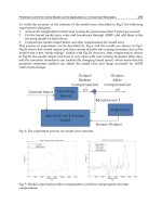
Closed-loop step responses for unconstrained and constrained cases are given in Fig.1 and
Fig.2, respectively. Closed-loop step responses for the case of in this chapter proposed algo-
rithm are given in Fig.3. Maximal value of control variable is about u
max
= 0.08 < 0.1.
Input constraints conditions were applied only for plant control variable u
(t).
Second example has been borrowed from (Camacho & Bordons (2004), p.147). The model cor-
responds to the longitudinal motion of a Boeing 747 airplane. The multivariable process is
controlled using a predictive controller based on the output model of the aircraft. Two of the
usual command outputs that must be controlled are airspeed that is, velocity with respect to
air, and climb rate. Continuous model has been converted to discrete time one with sampling
time of 0.1s, the nominal model turns to (1) where
A
o
=




.9996 .0383 .0131

−.0322
−.0056 .9647 .7446 .0001
.002
−.0097 .9543 0
.0001
−.0005 .0978 1




Robust Model Predictive Control Design 9
For gain matrices F
i
, i = 1, 2 we obtain two closed-loop system in the form (13), A
ci
= A
f
+
B
f
F
i
C
f
, i = 1, 2. Consider the edge between A
c1
and A
c2
, that is
A

c
= αA
c1
+ (1 − α)A
c2
, α ∈< 0, 1 > (30)
The following lemma gives the stability conditions for matrix A
c
(30).
Lemma 2. Consider the stable closed-loop system matrices A
ci
, i = 1, 2.
• If there exists a positive definite matrix P
q
such that
A
T
ci
P
q
A
ci
− P
q
≤ 0, i = 1, 2 (31)
then matrix A
c
(30) is quadratically stable.
• If there exist two positive definite matrices P
1

, P
2
such that they satisfy the parameter
dependent quadratic stability conditions, see (Peaucelle et al., 2000), (Grman et al., 2005)
the closed-loop system A
c
is parameter dependent quadratically stable (PDQS).
Remarks
• If closed-loop matrices A
ci
, i = 1, 2 satisfy (31) the scalar γ in (29) may be changed
with any rate without violating the closed-loop stability.
• If closed-loop matrices A
ci
, i = 1, 2 are PDQS, the scalar γ in (29) has to be constant
but may be unknown.
• The proposed control algorithm (29) is similar to Soft Variable-Structure Control (SVSC),
(Adamy & Fleming, 2004), but in our case, when
|v
i
| << U
i
the feedback gain matrix
F (29) gives rather quicker dynamic behavior of the closed-loop system (unconstrained
case) than when
|v
i
| approaches to U
i
.

Algorithm for calculation of γ for (29) may be as follows:
γ
= min
i
U
i
− |v
i
|
U
i
(32)
If accidentally some
|v
i
| > U
i
, γ = 0.
The resulting control design procedure is given by the next steps
• Off-line computation stage, compute output feedback gain matrices:
F
1
for unconstrained case as a solution to (20), where LMI (20) is solved for unknown P
and F;
F
2
for constrained case as a solution to (20) and (25).
• On-line computation- in each step:
compute the actual value of scalar parameter γ, e.g from (32) (where v
i

is obtained from
(12) for F
= F
1
;
compute the actual feedback gain matrix from (29) and respective constrained control
vector from (12). All on-line computations follow general MPC scheme, i.e. the first
part of computed control vector u
(t) is applied on real controlled plant and the other
part of control vector is used for model prediction.
1.4 EXAMPLES
Two examples are presented to illustrate the qualities of the control design procedure pro-
posed above, namely its ability to cope with robust stability and input constraints without
complex computational load. In each example the results of three simulation experiments are
compared for closed-loop with output feedback control:
case 1 Unconstrained case for output feedback gain matrix F
1
case 2 Constrained case for output feedback gain matrix F
2
case 3 The new proposed control algorithm (29) for output feedback gain matrix F.
The input constraint case is studied, in each case maximal value of u
(t) is checked; stability is
assessed using spectral radius of closed-loop system matrix.
First example serves as a benchmark. The model of double integrator turns to (1) where
A
o
=

1 0
1 1


B
o
=

1
0

, C
=

0 1

and uncertainty matrices are
A
1u
=

0.01 0.01
0.02 0.03

B
1u
=

0.001
0

,
For the case when number of uncertainty is p

= 1, the number of the respective polytope
vertices is N
= 2
p
= 2, the matrices (2) are calculated as follows
A
1
= A
o
− A
1u
, A
2
= A
o
+ A
1u
, B
1
= B
o
− B
1u
, B
2
= B
o
+ B
1u
For the parameters:  = 20000, N

2
= 6, N
u
= 6, Q
0
= 0.1I, Q
1
= 0.5I, Q
2
= = Q
6
= I, R =
I, the following results are obtained for unconstrained and constrained cases
• Unconstrained case: Closed
− loopmaxeig = 0.8495. Maximal value of control variable
is about u
max
= 0.24.
• Constrained case with U
i
= 0.1, θ = 1000, Closed − loopmaxeig = 0.9437. Maximal
value of control variable is about u
max
= 0.04.
Closed-loop step responses for unconstrained and constrained cases are given in Fig.1 and
Fig.2, respectively. Closed-loop step responses for the case of in this chapter proposed algo-
rithm are given in Fig.3. Maximal value of control variable is about u
max
= 0.08 < 0.1.
Input constraints conditions were applied only for plant control variable u

(t).
Second example has been borrowed from (Camacho & Bordons (2004), p.147). The model cor-
responds to the longitudinal motion of a Boeing 747 airplane. The multivariable process is
controlled using a predictive controller based on the output model of the aircraft. Two of the
usual command outputs that must be controlled are airspeed that is, velocity with respect to
air, and climb rate. Continuous model has been converted to discrete time one with sampling
time of 0.1s, the nominal model turns to (1) where
A
o
=




.9996 .0383 .0131
−.0322
−.0056 .9647 .7446 .0001
.002
−.0097 .9543 0
.0001
−.0005 .0978 1




Model Predictive Control10
Fig. 1. Dynamic behavior of controlled system for unconstrained case for u(t) .
B
o
=





.0001 .1002
−.0615 .0183
−.1133 .0586
−.0057 .0029




C
=

1 0 0 0
0
−1 0 7.74

and model uncertainty matrices are
A
1u
=




0 0 0 0
0 0.0005 0.0017 0
0 0 0.0001 0

0 0 0 0




B
1u
=




0 0.12
−0.02 0.1
−0.12 0
0 0




10
−3
For the case when number of uncertainty is p = 1, the number of vertices is N = 2
p
= 2, the
matrices (2) are calculated as in example 1. Note that nominal model A
o
is unstable. Consider
N
2

= N
u
= 1,  = 20000 and weighting matrices Q
0
= Q
1
= 1I, R
0
= R
1
= I the following
results are obtained:
• Unconstrained case: maximal closed-loop nominal model eigenvalue is Closed
− loopmaxeig =
0.9983. Maximal value of control variables are about u
1max
= 9.6, u
2max
= 6.3.
• Constrained case with U
i
= 1, θ = 40000 Closed − loopmaxeig = 0.9998 Maximal values
of control variables are about u
1max
= 0.21, u
2max
= 0.2.
Closed-loop nominal model step responses of the above two cases for the input u
(t) are given
in the Fig.4 and Fig.5, respectively. Closed-loop step responses for in the paper proposed

control algorithm (29) and (32) are in Fig.6. Maximal values of control variables are about
u
1max
= 0.75 < 1, u
2max
= 0.6 < 1. Input constraint conditions were applied only for plant
control variable u
(t). Both examples show that using tuning parameter θ the demanded input
Fig. 2. Dynamic behavior of controlled system for constrained case for u(t) .
constraints can be reached with high accuracy. The initial guess of θ can be obtained from (28).
It can be seen that the proposed control scheme provides reasonable results : the response in
case 3 (Fig.3 , Fig. 6) are quicker than those in case 2 (Fig.2, Fig.5), while the computation load
has not much increased comparing to case 2.
2. ROBUST MPC DESIGN: SEQUENTIAL APPROACH
2.1 INTRODUCTION
In this part a new MPC algorithm is proposed pursuing the idea of (Veselý & Rosinová ,
2009). The proposed robust MPC control algorithm is designed sequentially. The respec-
tive sequential robust MPC design procedure consists from two steps. In the first step and
one step ahead prediction horizon, the necessary and sufficient robust stability conditions
have been developed for MPC and polytopic system with output feedback, using generalized
parameter dependent Lyapunov matrix P
(α). The proposed robust MPC algorithm ensures
parameter dependent quadratic stability (PDQS) and guaranteed cost. In the second step of
design procedure, the nominal plant model is used to design the predicted input variables
u
(t + 1), u(t + N
2
− 1) so that the robust closed-loop stability of MPC and guaranteed cost
are ensured. Thus, input variable u
(t) guarantees the performance and robustness proper-

ties of closed-loop system and predicted input variables u
(t + 1), u(t + N
2
− 1) guarantee
the performance and closed-loop stability of uncertain plant model and nominal model pre-
diction. Note that within sequentially design procedure the degree of plant model does not
change when the output prediction horizon changes.
This part of chapter is organized as follows: Section 2.2 presents preliminaries and problem
formulation. In Section 2.3 the main results are given and finally, in Section 2.4 two examples
solved using Yalmip BMI solvers show the effectiveness of the proposed method.
Robust Model Predictive Control Design 11
Fig. 1. Dynamic behavior of controlled system for unconstrained case for u(t) .
B
o
=




.0001 .1002
−.0615 .0183
−.1133 .0586
−.0057 .0029




C
=


1 0 0 0
0
−1 0 7.74

and model uncertainty matrices are
A
1u
=




0 0 0 0
0 0.0005 0.0017 0
0 0 0.0001 0
0 0 0 0




B
1u
=




0 0.12
−0.02 0.1
−0.12 0

0 0




10
−3
For the case when number of uncertainty is p = 1, the number of vertices is N = 2
p
= 2, the
matrices (2) are calculated as in example 1. Note that nominal model A
o
is unstable. Consider
N
2
= N
u
= 1,  = 20000 and weighting matrices Q
0
= Q
1
= 1I, R
0
= R
1
= I the following
results are obtained:
• Unconstrained case: maximal closed-loop nominal model eigenvalue is Closed
− loopmaxeig =
0.9983. Maximal value of control variables are about u

1max
= 9.6, u
2max
= 6.3.
• Constrained case with U
i
= 1, θ = 40000 Closed − loopmaxeig = 0.9998 Maximal values
of control variables are about u
1max
= 0.21, u
2max
= 0.2.
Closed-loop nominal model step responses of the above two cases for the input u
(t) are given
in the Fig.4 and Fig.5, respectively. Closed-loop step responses for in the paper proposed
control algorithm (29) and (32) are in Fig.6. Maximal values of control variables are about
u
1max
= 0.75 < 1, u
2max
= 0.6 < 1. Input constraint conditions were applied only for plant
control variable u
(t). Both examples show that using tuning parameter θ the demanded input
Fig. 2. Dynamic behavior of controlled system for constrained case for u(t) .
constraints can be reached with high accuracy. The initial guess of θ can be obtained from (28).
It can be seen that the proposed control scheme provides reasonable results : the response in
case 3 (Fig.3 , Fig. 6) are quicker than those in case 2 (Fig.2, Fig.5), while the computation load
has not much increased comparing to case 2.
2. ROBUST MPC DESIGN: SEQUENTIAL APPROACH
2.1 INTRODUCTION

In this part a new MPC algorithm is proposed pursuing the idea of (Veselý & Rosinová ,
2009). The proposed robust MPC control algorithm is designed sequentially. The respec-
tive sequential robust MPC design procedure consists from two steps. In the first step and
one step ahead prediction horizon, the necessary and sufficient robust stability conditions
have been developed for MPC and polytopic system with output feedback, using generalized
parameter dependent Lyapunov matrix P
(α). The proposed robust MPC algorithm ensures
parameter dependent quadratic stability (PDQS) and guaranteed cost. In the second step of
design procedure, the nominal plant model is used to design the predicted input variables
u
(t + 1), u(t + N
2
− 1) so that the robust closed-loop stability of MPC and guaranteed cost
are ensured. Thus, input variable u
(t) guarantees the performance and robustness proper-
ties of closed-loop system and predicted input variables u
(t + 1), u(t + N
2
− 1) guarantee
the performance and closed-loop stability of uncertain plant model and nominal model pre-
diction. Note that within sequentially design procedure the degree of plant model does not
change when the output prediction horizon changes.
This part of chapter is organized as follows: Section 2.2 presents preliminaries and problem
formulation. In Section 2.3 the main results are given and finally, in Section 2.4 two examples
solved using Yalmip BMI solvers show the effectiveness of the proposed method.
Model Predictive Control12
Fig. 3. Dynamic behavior of controlled system with the proposed algorithm for u(t) .
2.2 PROBLEM FORMULATION AND PRELIMINARIES
For readers convenience, uncertain plant model and respective preliminaries are briefly re-
called. A time invariant linear discrete-time uncertain polytopic system is

x
(t + 1 ) = A(α )x(t) + B(α)u(t) (33)
y
(t) = Cx(t)
where x(t) ∈ R
n
, u(t) ∈ R
m
, y(t) ∈ R
l
are state, control and output variables of the system,
respectively; A
(α), B(α) belong to the convex set
S
= {A(α) ∈ R
n×n
, B(α) ∈ R
n×m
} (34)
{A(α) =
N
∑
j=1
A
j
α
j
B(α) =
N
∑

j=1
B
j
α
j
, α
j
≥ 0 }, j = 1, 2 N,
N
∑
j=1
α
j
= 1
Matrix C is constant known matrix of corresponding dimension. Jointly with the system (33),
the following nominal plant model will be used.
x
(t + 1 ) = A
o
x(t) + B
o
u(t) (35)
y
(t) = Cx(t)
where (A
o
, B
o
) ∈ S are any matrices with constant entries. The problem studied in this part
of chapter can be summarized as follows: in the first step, parameter dependent quadratic

stability conditions for output feedback and one step ahead robust model predictive control
are derived for the polytopic system (33), (34), when control algorithm is given as
u
(t) = F
11
y(t) + F
12
y(t + 1) (36)
and in the second step of design procedure, considering a nominal model (35) and a given
prediction horizon N
2
a model predictive control is designed in the form:
u
(t + k − 1) = F
kk
y(t + k − 1) + F
kk+1
y(t + k) (37)
Fig. 4. Dynamic behavior of unconstrained controlled system for u(t) .
where F
ki
∈ R
m×l
, k = 2, 3, N
2
; i = k + 1 are output (state) feedback gain matrices to be
determined so that cost function given below is optimal with respect to system variables. We
would like to stress that y
(t + k − 1), y(t + 1) are predicted outputs obtained from predictive
model (44).

Substituting control algorithm (36) to (33) we obtain
x
(t + 1 ) = D
1
(j)x(t) (38)
where
D
1
(j) = A
j
+ B
j
K
1
(j)
K
1
(j) = (I − F
12
CB
j
)
−1
(F
11
C + F
12
CA
j
), j = 1, 2, N

For the first step of design procedure, the cost function to be minimized is given as
J
1
=
∞
∑
t=0
J
1
(t) (39)
where
J
1
(t) = x(t)
T
Q
1
x(t) + u(t)
T
R
1
u(t)
and Q
1
, R
1
are positive definite matrices of corresponding dimensions. For the case of k = 2
we obtain
u
(t + 1 ) = F

22
CD
1
(j)x(t) + F
23
C(A
o
D
1
(j)x(t) + B
o
u(t + 1))
or
u
(t + 1 ) = K
2
(j)x(t)
and closed-loop system
x
(t + 2 ) = (A
o
D
1
(j) + B
o
K
2
(j))x(t) = D
2
(j)x(t), j = 1, 2, N