Model Predictive Control Part 7 potx

Model predictive control of nonlinear processes 113
time by an adaptive mechanism. The one step ahead predictive model can be recursively
extended to obtain future predictions for the plant output. The minimization of a cost
function based on future plant predictions and desired plant outputs generates an optimal
control input sequence to act on the plant. The strategy is described as follows.

Predictive model
The relation between the past input-output data and the predicted output can be expressed
by an ARX model of the form

y(t+1) = a
1
y(t) + . . . + a
ny
y(t-ny+1) + b
1
u(t) +. . . . . . . + b
nu
u(t-nu+1) (1)

where y(t) and u(t) are the process and controller outputs at time t, y(t+1) is the one-step
ahead model prediction at time t, a’s and b’s represent the model coefficients and the nu and
ny are input and output orders of the system.

Model identification

The model output prediction can be expressed as

y
m
(t+1) =


x
m
(t) (2)
where


= [

1
. . .

ny


1
. . .

nu
] (3)
and
x
m
(t) = [y(t) . . . y(t-ny+1)

u(t) . . . u(t-nu+1)]
T
(4)

with


and


as identified model parameters.
One of the most widely used estimators for model parameters and covariance is the popular
recursive least squares (RLS) algorithm (Goodwin and Sin, 1984). The RLS algorithm
provides the updated parameters of the ARX model in the operating space at each sampling
instant or these parameters can be determined a priori using the known data of inputs and
outputs for different operating conditions. The RLS algorithm is expressed as



(t+1) =

(t) + K(t) [y(t+1) - y
m
(t+1)]
K(t) = P(t) x
m
(t+1) / [1 + x
m
(t+1)
T
P(t) x
m
(t+1)] (5)
P(t+1) = 1/

[P(t) - {( P(t) x

m
(t+1) x
m
(t+1)
T
P(t)) / (1 + x
m
(t+1)
T
P(t) x
m
(t+1))}]

where

(t) represents the estimated parameter vector,

is the forgetting factor, K(t) is the
gain matrix and P(t) is the covariance matrix.

Controller formulation

The N time steps ahead output prediction over a prediction horizon is given by


1
( )
p
y t N


 
y(t+N-1)+ +

ny
y(t-ny+N)+

1
u(t+N-1)+ +

nu
u(t-nu+N)+err(t) (6)

where y
p
(t+N) represent the model predictions for N steps and err(t) is an estimate of the
modeling error which is assumed as constant for the entire prediction horizon. If the control
horizon is m, then the controller output, u after m time steps can be assumed to be constant.
An internal model is used to eliminate the discrepancy between model and process outputs,
error(t), at each sampling instant
error(t) = y(t) - y
m
(t) (7)

where y
m
(t) is the one-step ahead model prediction at time (t-1). The estimate of the error is
then filtered to produce err(t) which minimizes the instability introduced by the modeling
error feedback. The filter error is given by

err(t) = (1-K

f
) err(t-1) + K
f
error(t) (8)

where K
f
is the feedback filter gain which has to be tuned heuristically.
Back substitutions transform the prediction model equations into the following form


,1
, , 1
, 1
,1 ,
( ) ( )
( 1) ( 1)
( 1)
( ) ( 1)
( )
p N
N ny N ny
N ny nu
N N m
N
y t N f y t
f y t ny f u t
f u t nu
g u t g u t m
e err t


 
   
    
   
   

(9)
The elements f, g and e are recursively calculated using the parameters

and

of
Eq. (3). The above equations can be written in a condensed form as

Y(t) = F X(t) + G U(t) + E err(t) (10)

where
Y(t) = [y
p
(t+1) . . . y
p
(t+N)]
T
(11)


X(t) = [y(t) y(t-1) . . . y(t-ny+1) u(t-1) . . . u(t-nu+1)]
T
(12)

U(t) = [u(t) . . . u(t+m-1)]
T
(13)

11 12 1( 1)
11 12 2( 1)
1 12 ( 1)


:
:

ny nu
ny nu
N N N ny nu
f f f
f f f
F
f f f
 
 
 
 
 
 
 

 
 
 

 
 

11
21 21
1 2 3
1 2 3
0 0 0
0 0
. . . . .

. . . . .
. . . . .

. . . .
. . . .

. . . .

m m m mm
N N N Nm
g
g g
G
g g g g
g g g g
 
 
 
 

 
 
 
 

 
 
 
 
 
 
 
 

E = [e
1
. . . e
N
]
T

Model Predictive Control114
In the above, Y(t) represents the model predictions over the prediction horizon, X(t) is a
vector of past plant and controller outputs and U(t) is a vector of future controller outputs. If
the coefficients of F, G and E are determined then the transformation can be completed. The
number of columns in F is determined by the ARX model structure used to represent the
system, where as the number of columns in G is determined by the length of the control
horizon. The number of rows is fixed by the length of the prediction horizon.

Consider a cost function of the form

 
2
2
1 1
( ) ( ) ( 1
N m
p
i i
J y t i w t i u t i

 
 
      
 
 


   
1 1
( ) ( ) ( ) ( ) ( ) ( )
N m
T
T
i i
Y t W t Y t W t U t U t

 
   
 

(14)
where W(t) is a setpoint vector over the prediction horizon

W(t) = [ w(t+1) . . . . w(t+N)]
T
(15)


The minimization of the cost function, J gives optimal controller output sequence

U(t) = [G
T
G +

I ]
-1
G
T
[W(t) - FX(t) - Eerr(t)] (16)


The vector U(t) generates control sequence over the entire control horizon. But, the first
component of U(t) is actually implemented and the whole procedure is repeated again at the
next sampling instant using latest measured information.
Linear model predictive control involving input-output models in classical, adaptive or
fuzzy forms is proved useful for controlling processes that exhibit even some degree of
nonlinear behavior (Eaton and Rawlings, 1992; Venkateswarlu and Gangiah, 1997 ;
Venkateswarlu and Naidu, 2001).

3.2 Case study: linear model predictive control of a reactive distillation column

In this study, a multistep linear model predictive control (LMPC) strategy based on
autoregressive moving average (ARX) model structure is presented for the control of a
reactive distillation column. Although MPC has been proved useful for a variety of chemical
and biochemical processes (Garcia et al., 1989 ; Eaton and Rawlings, 1992), its application to
a complex dynamic system like reactive distillation is more interesting.

The process and the model
Ethyl acetate is produced through an esterfication reaction between acetic acid and ethyl
alcohol

5232523
HCOOCCHOHOHHCCOOHCH
H
 

(17)

The achievable conversion in this reversible reaction is limited by the equilibrium
conversion. This quaternary system is highly non-ideal and forms binary and ternary
azeotropes, which introduce complexity to the separation by conventional distillation.
Reactive distillation can provide a means of breaking the azeotropes by altering or
eliminating the conditions for azeotrope formation. Thus reactive distillation becomes
attractive alternative for the production of ethyl acetate.
The rate equation of this reversible reaction in the presence of a homogeneous acid catalyst
is given by (Alejski and Duprat, 1996)


1
1 1 1 2 3 4
1

6500.1
(4.195 0.08815)exp( )
7.558 0.012
c
k
c
k
r k C C C C
K
k C
T
K T
 
  
 
(18)

Vora and Daoutidis (2001) have presented a two feed column configuration for ethyl acetate
reactive distillation and found that by feeding the two reactants, ethanol and acetic acid, on
different trays counter currently allows to enhance the forward reaction on trays and results
in higher conversion and purity over the conventional column configuration of feeding the
reactants on a single tray. All plates in the column are considered to be reactive. The column
consists of 13 stages including the reboiler and the condenser. The less volatile acetic acid
enters the 3 rd tray and the more volatile ethanol enters the 10 th tray. The steady state
operating conditions of the column are shown in Table 1.


Acetic acid feed flow rate, F
Ac
6.9 mol/s

Ethanol flow rate, F
Eth
6.865 mol/s
Reflux flow rate, L
o
13.51 mol/s
Distillate flow rate, D 6.68 mol/s
Bottoms flow rate, B 7.085 mol/s
Reboiler heat duty, Q
r
5.88 x 10
5
J/mol
Boiling points,
o
K 391.05, 351.45, 373.15, 350.25
(Acetic acid, ethanol, water, ethyl acetate)
Distillate composition 0.0842, 0.1349, 0.0982, 0.6827
(Acetic acid, ethanol, water, ethyl acetate)
Bottoms composition 0.1650, 0.1575, 0.5470, 0.1306
(Acetic acid, ethanol, water, ethyl acetate)

Table 1. Design conditions for ethyl acetate reactive distillation column

The dynamic model representing the process operation involves mass and component
balance equations with reaction terms, along with energy equations supported by vapor-
liquid equilibrium and physical properties (Alejski & Duprat, 1996). The assumptions made
in the formulation of the model include adiabatic column operation, negligible heat of
reaction, negligible vapor holdup, liquid phase reaction, physical equilibrium in streams
leaving each stage, negligible down comer dynamics and negligible weeping of liquid

through the openings on the tray surface. The equations representing the process are given
as follows.
Model predictive control of nonlinear processes 115
In the above, Y(t) represents the model predictions over the prediction horizon, X(t) is a
vector of past plant and controller outputs and U(t) is a vector of future controller outputs. If
the coefficients of F, G and E are determined then the transformation can be completed. The
number of columns in F is determined by the ARX model structure used to represent the
system, where as the number of columns in G is determined by the length of the control
horizon. The number of rows is fixed by the length of the prediction horizon.

Consider a cost function of the form

 
2
2
1 1
( ) ( ) ( 1
N m
p
i i
J y t i w t i u t i

 
 
      
 
 


   

1 1
( ) ( ) ( ) ( ) ( ) ( )
N m
T
T
i i
Y t W t Y t W t U t U t

 
   
 
(14)
where W(t) is a setpoint vector over the prediction horizon

W(t) = [ w(t+1) . . . . w(t+N)]
T
(15)


The minimization of the cost function, J gives optimal controller output sequence

U(t) = [G
T
G +

I ]
-1
G
T
[W(t) - FX(t) - Eerr(t)] (16)

The vector U(t) generates control sequence over the entire control horizon. But, the first
component of U(t) is actually implemented and the whole procedure is repeated again at the
next sampling instant using latest measured information.
Linear model predictive control involving input-output models in classical, adaptive or
fuzzy forms is proved useful for controlling processes that exhibit even some degree of
nonlinear behavior (Eaton and Rawlings, 1992; Venkateswarlu and Gangiah, 1997 ;
Venkateswarlu and Naidu, 2001).

3.2 Case study: linear model predictive control of a reactive distillation column
In this study, a multistep linear model predictive control (LMPC) strategy based on
autoregressive moving average (ARX) model structure is presented for the control of a
reactive distillation column. Although MPC has been proved useful for a variety of chemical
and biochemical processes (Garcia et al., 1989 ; Eaton and Rawlings, 1992), its application to
a complex dynamic system like reactive distillation is more interesting.

The process and the model
Ethyl acetate is produced through an esterfication reaction between acetic acid and ethyl
alcohol

5232523
HCOOCCHOHOHHCCOOHCH
H
 

(17)

The achievable conversion in this reversible reaction is limited by the equilibrium
conversion. This quaternary system is highly non-ideal and forms binary and ternary

azeotropes, which introduce complexity to the separation by conventional distillation.
Reactive distillation can provide a means of breaking the azeotropes by altering or
eliminating the conditions for azeotrope formation. Thus reactive distillation becomes
attractive alternative for the production of ethyl acetate.
The rate equation of this reversible reaction in the presence of a homogeneous acid catalyst
is given by (Alejski and Duprat, 1996)


1
1 1 1 2 3 4
1
6500.1
(4.195 0.08815)exp( )
7.558 0.012
c
k
c
k
r k C C C C
K
k C
T
K T
 
  
 
(18)

Vora and Daoutidis (2001) have presented a two feed column configuration for ethyl acetate
reactive distillation and found that by feeding the two reactants, ethanol and acetic acid, on

different trays counter currently allows to enhance the forward reaction on trays and results
in higher conversion and purity over the conventional column configuration of feeding the
reactants on a single tray. All plates in the column are considered to be reactive. The column
consists of 13 stages including the reboiler and the condenser. The less volatile acetic acid
enters the 3 rd tray and the more volatile ethanol enters the 10 th tray. The steady state
operating conditions of the column are shown in Table 1.


Acetic acid feed flow rate, F
Ac
6.9 mol/s
Ethanol flow rate, F
Eth
6.865 mol/s
Reflux flow rate, L
o
13.51 mol/s
Distillate flow rate, D 6.68 mol/s
Bottoms flow rate, B 7.085 mol/s
Reboiler heat duty, Q
r
5.88 x 10
5
J/mol
Boiling points,
o
K 391.05, 351.45, 373.15, 350.25
(Acetic acid, ethanol, water, ethyl acetate)
Distillate composition 0.0842, 0.1349, 0.0982, 0.6827
(Acetic acid, ethanol, water, ethyl acetate)

Bottoms composition 0.1650, 0.1575, 0.5470, 0.1306
(Acetic acid, ethanol, water, ethyl acetate)

Table 1. Design conditions for ethyl acetate reactive distillation column

The dynamic model representing the process operation involves mass and component
balance equations with reaction terms, along with energy equations supported by vapor-
liquid equilibrium and physical properties (Alejski & Duprat, 1996). The assumptions made
in the formulation of the model include adiabatic column operation, negligible heat of
reaction, negligible vapor holdup, liquid phase reaction, physical equilibrium in streams
leaving each stage, negligible down comer dynamics and negligible weeping of liquid
through the openings on the tray surface. The equations representing the process are given
as follows.
Model Predictive Control116

Total mass balance
Total condenser:

112
1
)( RDLV
dt
dM
 (19)
Plate j:

jjjjjjj
j
RLVLFLVFV
dt

dM

 11
(20)
Reboiler :

nnnn
n
RLVL
dt
dM

1
(21)
Component mass balance
Total condenser :

1,1,12,2
1,1
)(
)(
iii
i
RxDLyV
dt
xMd

(22)
Plate j:

,
, 1 , 1 , 1 , 1 , , ,
( )
j i j
j i j j i j j i j j i j j i j j i j i j
d M x
FV yf V y FL xf L x V y L x R
dt
   
      
(23)
Reboiler:

,
1 , 1 , , ,
( )
n i n
n i n n i n n i n i n
d M x
L x V y L x R
dt
 
    (24)

Total energy balance
Total condenser :

11122
1
)( QhDLHV

dt
dE
 (25)
Plate j:

jjjjjjjjjjjjj
j
QhLHVhLhfFLHVHfFV
dt
dE

 1111
(26)

Reboiler:

nnnnnnn
n
QhLHVhL
dt
dE

 11
(27)
Level of liquid on the tray

avtray
avn
liq
A

MWM
L

 (28)
Flow of liquid over the weir
If ( L
liq
<h
weir
) then L
n
= 0 (29)

else

2
3
)(84.1
weir
liq
av
avweir
n
hL
MW
L
L 

(30)
Mole fraction normalization

1
11



NC
i
i
NC
i
i
yx
(31)

VLE calculations

For the column operation under moderate pressures, the VLE equation assumes the ideal
gas model for the vapor phase, thus making the vapor phase activity coefficient equal to
unity. The VLE relation is given by

y
i
P = x
i


i
P

i
sat
(i = 1,2,….,NC) (32)

The liquid phase activity coefficients are calculated using UNIFAC method (Smith et al.,
1996).

Enthalpies Calculation
The relations for the liquid enthalpy h, the vapor enthalpy H and the liquid density

are:


),,(
),,(
),,(
xTP
yTPHH
xTPhh
liqliq




(33)

Control scheme

The design and implementation of the control strategy is studied for the single input-single
output (SISO) control of the ethyl acetate reactive distillation column with its double feed

configuration. The objective is to control the desired product purity in the distillate stream
inspite disturbances in column operation. This becomes the main control loop. Since reboiler
and condenser holdups act as pure integrators, they also need to be controlled. These
become the auxiliary control loops. Reflux flow rate is used as a manipulated variable to
control the purity of the ethyl acetate. Distillate flow rate is used as a manipulated variable
to control the condenser holdup, while bottom flow rate is used to control the reboiler
holdup. In this work, it is proposed to apply a multistep model predictive controller for the
main loop and conventional PI controllers for the auxiliary control loops. This control
scheme is shown in the Figure 3.

Model predictive control of nonlinear processes 117

Total mass balance
Total condenser:

112
1
)( RDLV
dt
dM
 (19)
Plate j:

jjjjjjj
j
RLVLFLVFV
dt
dM

 11

(20)
Reboiler :

nnnn
n
RLVL
dt
dM

1
(21)
Component mass balance
Total condenser :

1,1,12,2
1,1
)(
)(
iii
i
RxDLyV
dt
xMd

(22)
Plate j:

,
, 1 , 1 , 1 , 1 , , ,
( )

j i j
j i j j i j j i j j i j j i j j i j i j
d M x
FV yf V y FL xf L x V y L x R
dt
   
      
(23)
Reboiler:

,
1 , 1 , , ,
( )
n i n
n i n n i n n i n i n
d M x
L x V y L x R
dt
 
    (24)

Total energy balance
Total condenser :

11122
1
)( QhDLHV
dt
dE
 (25)

Plate j:

jjjjjjjjjjjjj
j
QhLHVhLhfFLHVHfFV
dt
dE

 1111
(26)

Reboiler:

nnnnnnn
n
QhLHVhL
dt
dE

 11
(27)
Level of liquid on the tray

avtray
avn
liq
A
MWM
L


 (28)
Flow of liquid over the weir
If ( L
liq
<h
weir
) then L
n
= 0 (29)

else

2
3
)(84.1
weir
liq
av
avweir
n
hL
MW
L
L 

(30)
Mole fraction normalization


1

11



NC
i
i
NC
i
i
yx
(31)

VLE calculations

For the column operation under moderate pressures, the VLE equation assumes the ideal
gas model for the vapor phase, thus making the vapor phase activity coefficient equal to
unity. The VLE relation is given by

y
i
P = x
i


i
P
i
sat
(i = 1,2,….,NC) (32)

The liquid phase activity coefficients are calculated using UNIFAC method (Smith et al.,
1996).

Enthalpies Calculation
The relations for the liquid enthalpy h, the vapor enthalpy H and the liquid density

are:


),,(
),,(
),,(
xTP
yTPHH
xTPhh
liqliq




(33)

Control scheme

The design and implementation of the control strategy is studied for the single input-single
output (SISO) control of the ethyl acetate reactive distillation column with its double feed
configuration. The objective is to control the desired product purity in the distillate stream
inspite disturbances in column operation. This becomes the main control loop. Since reboiler
and condenser holdups act as pure integrators, they also need to be controlled. These

become the auxiliary control loops. Reflux flow rate is used as a manipulated variable to
control the purity of the ethyl acetate. Distillate flow rate is used as a manipulated variable
to control the condenser holdup, while bottom flow rate is used to control the reboiler
holdup. In this work, it is proposed to apply a multistep model predictive controller for the
main loop and conventional PI controllers for the auxiliary control loops. This control
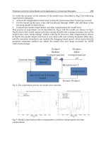
scheme is shown in the Figure 3.

Model Predictive Control118

Fig. 3. Control structure of two feed ethyl acetate reactive distillation column.

Analysis of Results
The performance of the multistep linear model predictive controller (LMPC) is evaluated
through simulation. The product composition measurements are obtained by solving the
model equations using Euler’s integration with sampling time of 0.01 s. The input and
output orders of the predictive model are considered as n
u
= 2 and n
y
= 2. The diagonal
elements of the initial covariance matrix, P(0) in the RLS algorithm are selected as 10.0, 1.0,
0.01, 0.01, respectively. The forgetting factor,  used in recursive least squares is chosen as
5.0. The feedback controller gain K
f
is assigned as 0.65. The tuning parameter

in the
control law is set as 0.115 x 10
-6
. The PI controller parameters of ethyl acetate composition

are evaluated by using the continuous cycling method of Ziegler and Nichols. The tuned
controller settings are k
c
= 11.15 and
I

= 1.61 x 10
4
s. The PI controller parameters used for
reflux drum and reboiler holdups are k
c
= - 0.001 and
I

= 5.5 h, and k
c
= - 0.001 and
I

= 5.5 h, respectively (Vora and Daoutidis, 2001).
The LMPC is implemented by adaptively updating the prediction model using recursive
least squares. On evaluating the effect of different prediction and control horizons, it is
observed that the LMPC with a prediction horizon of around 5 and a control horizon of 2
has shown reasonably better control performance. The LMPC is also referred here as MPC.
Figure 4 shows the results of MPC and PI controller when they are applied for tracking
series of step changes in ethyl acetate composition. The regulatory control performance of
MPC and PI controller for 20% decrease in feed rate of acetic acid is shown in Figure 5. The
results thus show the effectiveness of the multistep linear model predictive control strategy
for the control of highly nonlinear reactive distillation column.

Fig. 4. Performance of MPC and PI controller for tracking series of step changes in distillate
composition.


Fig.5. Output and input profiles for MPC and PI controller for 20% decrease in the feed rate
of acetic acid.
Model predictive control of nonlinear processes 119

Fig. 3. Control structure of two feed ethyl acetate reactive distillation column.

Analysis of Results
The performance of the multistep linear model predictive controller (LMPC) is evaluated
through simulation. The product composition measurements are obtained by solving the
model equations using Euler’s integration with sampling time of 0.01 s. The input and
output orders of the predictive model are considered as n
u
= 2 and n
y
= 2. The diagonal
elements of the initial covariance matrix, P(0) in the RLS algorithm are selected as 10.0, 1.0,
0.01, 0.01, respectively. The forgetting factor,  used in recursive least squares is chosen as
5.0. The feedback controller gain K
f
is assigned as 0.65. The tuning parameter

in the
control law is set as 0.115 x 10
-6
. The PI controller parameters of ethyl acetate composition
are evaluated by using the continuous cycling method of Ziegler and Nichols. The tuned

controller settings are k
c
= 11.15 and
I

= 1.61 x 10
4
s. The PI controller parameters used for
reflux drum and reboiler holdups are k
c
= - 0.001 and
I

= 5.5 h, and k
c
= - 0.001 and
I

= 5.5 h, respectively (Vora and Daoutidis, 2001).
The LMPC is implemented by adaptively updating the prediction model using recursive
least squares. On evaluating the effect of different prediction and control horizons, it is
observed that the LMPC with a prediction horizon of around 5 and a control horizon of 2
has shown reasonably better control performance. The LMPC is also referred here as MPC.
Figure 4 shows the results of MPC and PI controller when they are applied for tracking
series of step changes in ethyl acetate composition. The regulatory control performance of
MPC and PI controller for 20% decrease in feed rate of acetic acid is shown in Figure 5. The
results thus show the effectiveness of the multistep linear model predictive control strategy
for the control of highly nonlinear reactive distillation column.

Fig. 4. Performance of MPC and PI controller for tracking series of step changes in distillate

composition.


Fig.5. Output and input profiles for MPC and PI controller for 20% decrease in the feed rate
of acetic acid.
Model Predictive Control120
4. Generalized predictive control
The generalized predictive control (GPC) is a general purpose multi-step predictive control
algorithm (Clarke et al., 1987) for stable control of processes with variable parameters,
variable dead time and a model order which changes instantaneously. GPC adopts an
integrator as a natural consequence of its assumption about the basic plant model. Although
GPC is capable of controlling such systems, the control performance of GPC needs to be
ascertained if the process constraints are to be encountered in nonlinear processes. Camacho
(1993) proposed a constrained generalized predictive controller (CGPC) for linear systems
with constrained input and output signals. By this strategy, the optimum values of the
future control signals are obtained by transforming the quadratic optimization problem into
a linear complementarity problem. Camacho demonstrated the results of the CGPC strategy
by carrying out a simulation study on a linear system with pure delay. Clarke et al. (1987)
have applied the GPC to open-loop stable unconstrained linear systems. Camacho applied
the CGPC to constrained open-loop stable linear system. However, most of the real
processes are nonlinear and some processes change behavior over a period of time.
Exploring the application of GPC to nonlinear process control will be more interesting.
In this study, a constrained generalized predictive control (CGPC) strategy is presented and
applied for the control of highly nonlinear and open-loop unstable processes with multiple
steady states. Model parameters are updated at each sampling time by an adaptive
mechanism.

4.1 GPC design
A nonlinear plant generally admits a local-linearized model when considering regulation
about a particular operating point. A single-input single-output (SISO) plant on linearization

can be described by a Controlled Autoregressive Integrated Moving Average (CARIMA)
model of the form
A(q
-1
)y(t) = B(q
-1
)q
-d
u(t) + C (q
-1
)e(t )/ (34)

where A, B and C are polynomials in the backward shift operator q
-1
. The y(t) is the
measured plant output, u(t) is the controller output, e(t) is the zero mean random Gaussian
noise, d is the delay time of the system and  is the differencing operator 1-q
-1
.
The control law of GPC is based on the minimization of a multi-step quadratic cost function
defined in terms of the sum of squares of the errors between predicted and desired output
trajectories with an additional term weighted by projected control increments as given by



3
2
1
2 2
1 2 3

1
( , , ) [ ( | ) ( )] [ ( 1)]
N
N
j N j
J N N N E y t j t w t j u t j

 


 
       
 
 


 
(35)

where E{.} is the expectation operator, y(t + j| t ) is a sequence of predicted outputs, w(t + j)
is a sequence of future setpoints, u(t + j -1) is a sequence of predicted control increments
and

is the control weighting factor. The N
1
, N
2
and N
3
are the minimum costing horizon,

the maximum costing horizon and the control horizon, respectively. The values of N
1
, N
2

and N
3
of Eq. (35) can be defined by N
1
= d + 1, N
2
= d + N, and N
3
= N, respectively.
Predicting the output response over a finite horizon beyond the dead-time of the process
enables the controller to compensate for constant or variable time delays. The recursion of
the Diophantine equation is a computationally efficient approach for modifying the
predicted output trajectory. An optimum j-step a head prediction output is given by

y(t + j| t) = G
j
(q
-1
) u(t + j - d - 1) + F
j
(q
-1
)y(t) (36)

where G

j
(q
-1
) = E
j
(q
-1
)B(q
-1
), and E
j
and F
j
are polynomials obtained recursively solving the
Diophantine equation,


)()(1
11 
 qFqAqE
j
j
j
(37)

The j-step ahead optimal predictions of y for j = 1, . . . , N
2
can be written in condensed form

Y =Gu + f (38)

where f contains predictions based on present and past outputs up to time t and past inputs
and referred to free response of the system, i.e., f = [f
1
, f
2
, … , f
N
]. The vector u corresponds
to the present and future increments of the control signal, i.e., u = [u(t), u(t+1), …….,
u(t+N-1)]
T
. Eq. (35) can be written as






uuwfGuwfGuJ
T
T


 (39)

The minimization of J gives unconstrained solution to the projected control vector

)()(
1

fwGIGGu
TT



(40)

The first component of the vector u is considered as the current control increment u(t),
which is applied to the process and the calculations are repeated at the next sampling
instant. The schematic of GPC control law is shown in Figure 6, where K is the first row of
the matrix
1
( )
T T
G G I G


 .

Fig. 6. The GPC control law
-
+
w
f
y(t)


u(t)
K

Process

Free response
of system
Model predictive control of nonlinear processes 121
4. Generalized predictive control
The generalized predictive control (GPC) is a general purpose multi-step predictive control
algorithm (Clarke et al., 1987) for stable control of processes with variable parameters,
variable dead time and a model order which changes instantaneously. GPC adopts an
integrator as a natural consequence of its assumption about the basic plant model. Although
GPC is capable of controlling such systems, the control performance of GPC needs to be
ascertained if the process constraints are to be encountered in nonlinear processes. Camacho
(1993) proposed a constrained generalized predictive controller (CGPC) for linear systems
with constrained input and output signals. By this strategy, the optimum values of the
future control signals are obtained by transforming the quadratic optimization problem into
a linear complementarity problem. Camacho demonstrated the results of the CGPC strategy
by carrying out a simulation study on a linear system with pure delay. Clarke et al. (1987)
have applied the GPC to open-loop stable unconstrained linear systems. Camacho applied
the CGPC to constrained open-loop stable linear system. However, most of the real

processes are nonlinear and some processes change behavior over a period of time.
Exploring the application of GPC to nonlinear process control will be more interesting.
In this study, a constrained generalized predictive control (CGPC) strategy is presented and
applied for the control of highly nonlinear and open-loop unstable processes with multiple
steady states. Model parameters are updated at each sampling time by an adaptive
mechanism.

4.1 GPC design
A nonlinear plant generally admits a local-linearized model when considering regulation
about a particular operating point. A single-input single-output (SISO) plant on linearization
can be described by a Controlled Autoregressive Integrated Moving Average (CARIMA)
model of the form
A(q
-1
)y(t) = B(q
-1
)q
-d
u(t) + C (q
-1
)e(t )/ (34)

where A, B and C are polynomials in the backward shift operator q
-1
. The y(t) is the
measured plant output, u(t) is the controller output, e(t) is the zero mean random Gaussian
noise, d is the delay time of the system and  is the differencing operator 1-q
-1
.
The control law of GPC is based on the minimization of a multi-step quadratic cost function

defined in terms of the sum of squares of the errors between predicted and desired output
trajectories with an additional term weighted by projected control increments as given by



3
2
1
2 2
1 2 3
1
( , , ) [ ( | ) ( )] [ ( 1)]
N
N
j N j
J N N N E y t j t w t j u t j

 




       






 

(35)

where E{.} is the expectation operator, y(t + j| t ) is a sequence of predicted outputs, w(t + j)
is a sequence of future setpoints, u(t + j -1) is a sequence of predicted control increments
and

is the control weighting factor. The N
1
, N
2
and N
3
are the minimum costing horizon,
the maximum costing horizon and the control horizon, respectively. The values of N
1
, N
2

and N
3
of Eq. (35) can be defined by N
1
= d + 1, N
2
= d + N, and N
3
= N, respectively.
Predicting the output response over a finite horizon beyond the dead-time of the process
enables the controller to compensate for constant or variable time delays. The recursion of
the Diophantine equation is a computationally efficient approach for modifying the

predicted output trajectory. An optimum j-step a head prediction output is given by

y(t + j| t) = G
j
(q
-1
) u(t + j - d - 1) + F
j
(q
-1
)y(t) (36)

where G
j
(q
-1
) = E
j
(q
-1
)B(q
-1
), and E
j
and F
j
are polynomials obtained recursively solving the
Diophantine equation,

)()(1
11 
 qFqAqE
j
j
j
(37)

The j-step ahead optimal predictions of y for j = 1, . . . , N
2
can be written in condensed form

Y =Gu + f (38)

where f contains predictions based on present and past outputs up to time t and past inputs
and referred to free response of the system, i.e., f = [f
1
, f
2
, … , f
N
]. The vector u corresponds
to the present and future increments of the control signal, i.e., u = [u(t), u(t+1), …….,
u(t+N-1)]
T
. Eq. (35) can be written as







uuwfGuwfGuJ
T
T


 (39)

The minimization of J gives unconstrained solution to the projected control vector

)()(
1
fwGIGGu
TT



(40)

The first component of the vector u is considered as the current control increment u(t),
which is applied to the process and the calculations are repeated at the next sampling
instant. The schematic of GPC control law is shown in Figure 6, where K is the first row of
the matrix
1
( )
T T
G G I G



 .












Fig. 6. The GPC control law
-
+
w
f
y(t)

u(t)
K

Process

Free response
of system
Model Predictive Control122
4.2 Constrained GPC design
In practice, all processes are subject to constraints. Control valves are limited by fully closed

and fully open positions and maximum slew rates. Constructive and safety reasons as well
as sensor ranges cause limits in process variables. Moreover, the operating points of plants
are
determined in order to satisfy economic goals and usually lie at the intersection of
certain constraints. Thus, the constraints acting on a process can be manipulated variable
limits (u
min
, u
max
), slew rate limits of the actuator (du
min
, du
max
), and limits on the output
signal (y
min
, y
max
) as given by


maxmin
)( utuu 

maxmin
)1()( dututudu  (41)

maxmin
)( ytyy 

These constraints can be expressed as


maxmin
)1( lultuTulu 

maxmin
lduuldu  (42)

maxmin
lyfGuly 

where l is an N vector containing ones, and T is an N x N lower triangular matrix containing
ones. By defining a new vector x = u - ldu
min
, the constrained equations can be transformed
as


cRx
x

 0
(43)
with

max min
max min
min min
max min

min min
( )
( 1)

; ( 1)
NxN
I l du du
T lu Tldu u t l
R T c lu Tldu u t l
G ly f Gldu
G ly f Gldu

   
   
  
   
   
      
   
 
   
   
   
   
(44)

Eq. (39) can be expressed as


o

T
fbuHuuJ 
2
1
(45)
where

)()(
)()(
)(2
wfwff
GwfwfGb
IGGH
T
o
TT
T






The minimization of J with no constraints on the control signal gives


bHu
1
 (46)
Eq. (45) in terms of the newly defined vector x becomes

1
2
1
faxHxxJ
T
 (47)
where

min
2
min1
min
2
1
blduHllduff
Hluba
T
o
T



The solution of the problem can be obtained by minimization of Eq. (47) subject to the
constraints of Eq. (43). By using the Lagrangian multiplier vectors v
1
and v for the
constraints, x ≥ 0 and Rx ≤ c, respectively, and introducing the slack variable vector v
2
, the

Kuhn-Tucker conditions can be expressed as


0,,,
0
0
21
2
1
1
2





vvvx
vv
vx
avvRHx
cvRx
T
T
T
(48)

Camacho (1993) has proposed the solution of this problem with the help of Lemke’s
algorithm (Bazaraa and Shetty, 1979) by expressing the Kuhn-Tucker conditions as a linear
complementarity problem starting with the following tableau

min
11
min2
11
2
012
1
1

xHRHIOx
vRHRRHOIv
zvvxv
T
NxNNxm
T
mxNmxn




(49)

Here, z
0
is the artificial variable which will be driven to zero iteratively.

In this study, the above stated constrained generalized predictive linear control of Camacho
(1993)

is extended to open-loop unstable constrained control of nonlinear processes. In this
Model predictive control of nonlinear processes 123
4.2 Constrained GPC design
In practice, all processes are subject to constraints. Control valves are limited by fully closed
and fully open positions and maximum slew rates. Constructive and safety reasons as well
as sensor ranges cause limits in process variables. Moreover, the operating points of plants
are
determined in order to satisfy economic goals and usually lie at the intersection of
certain constraints. Thus, the constraints acting on a process can be manipulated variable
limits (u
min
, u
max
), slew rate limits of the actuator (du
min
, du
max
), and limits on the output
signal (y
min
, y
max
) as given by


maxmin
)( utuu



maxmin
)1()( dututudu




(41)

maxmin
)( ytyy




These constraints can be expressed as


maxmin
)1( lultuTulu






maxmin
lduuldu



(42)

maxmin
lyfGuly





where l is an N vector containing ones, and T is an N x N lower triangular matrix containing
ones. By defining a new vector x = u - ldu
min
, the constrained equations can be transformed
as


cRx
x

 0
(43)
with

max min
max min
min min
max min
min min
( )
( 1)

; ( 1)
NxN
I l du du
T lu Tldu u t l
R T c lu Tldu u t l
G ly f Gldu
G ly f Gldu


  

  
  

  

  
      

  
 

  

  
   

  
(44)

Eq. (39) can be expressed as


o
T
fbuHuuJ 
2
1
(45)
where

)()(
)()(
)(2
wfwff
GwfwfGb
IGGH
T
o
TT
T






The minimization of J with no constraints on the control signal gives

bHu
1
 (46)
Eq. (45) in terms of the newly defined vector x becomes

1
2
1
faxHxxJ
T
 (47)
where

min
2
min1
min
2
1
blduHllduff
Hluba
T
o
T



The solution of the problem can be obtained by minimization of Eq. (47) subject to the
constraints of Eq. (43). By using the Lagrangian multiplier vectors v

1
and v for the
constraints, x ≥ 0 and Rx ≤ c, respectively, and introducing the slack variable vector v
2
, the
Kuhn-Tucker conditions can be expressed as


0,,,
0
0
21
2
1
1
2





vvvx
vv
vx
avvRHx
cvRx
T
T
T
(48)

Camacho (1993) has proposed the solution of this problem with the help of Lemke’s
algorithm (Bazaraa and Shetty, 1979) by expressing the Kuhn-Tucker conditions as a linear
complementarity problem starting with the following tableau


min
11
min2
11
2
012
1
1

xHRHIOx
vRHRRHOIv
zvvxv
T
NxNNxm
T
mxNmxn




(49)

Here, z
0

is the artificial variable which will be driven to zero iteratively.

In this study, the above stated constrained generalized predictive linear control of Camacho
(1993)

is extended to open-loop unstable constrained control of nonlinear processes. In this
Model Predictive Control124
strategy, process nonlinearities are accounted through adaptation of model parameters
while taking care of input and output constraints acting on the process. The following
recursive least squares formula (Hsia, 1977) is used for on-line estimation of parameters and
the covariance matrix after each new sample:




)()1()1()1()()1()()1( kkkykkPkkk
T






 
)1()()1(1
1
)1(
)()1()1()()1()(
1
)1(




kkPk
k
kPkkkPkkPkP
T
T




(50)
where θ is the parameter vector, γ is the intermediate estimation variable, P is the covariance
matrix, v is the vector of input-output variables, y is the output variable, and 0 <

< 1 is the
forgetting factor. The initial covariance matrix and exponential forgetting factor are selected
based on various trials so as to provide reasonable convergence in parameter estimates.

The CGPC strategy of nonlinear processes is described in the following steps:

1. Specify the controller design parameters N
1
, N
2
, N
3
and also the initial parameter
estimates and covariance matrix for recursive identification of model parameters.

2. Update the model parameters using recursive least squares method.
3. Initialize the polynomials E
1
and F
1
of Diophantine identity, Eq. (37), using the estimated
parameters. Further initialize G
1
as E
1
B.
4. Compute the polynomials E
j
, F
j
and G
j
over the prediction horizon and control horizon
using the recursion of Diophantine.
5. Compute matrices H, R, and G, and vectors f and c using the polynomials determined in
step 4.
6. Compute the unconstrained solution x
min
= - H
-1
a.
7. Compute v
2min
= c - Rx
min

. If x
min
and v
2min
are nonnegative, then go to step 10.
8. Start Lemke’s algorithm with x and v
2
in the basis with the tableau, Eq. (49).
9. If x
1
is not in the first column of the tableau, make it zero; otherwise, assign it the
corresponding value.
10. Compute u(t) = x
1
+ du
min
+ u(t - 1).
11. Implement the control action, then shift to the next sampling instant and go to step 2.

4.3 Case study: constrained generalized predictive control (CGPC) of open-loop
unstable CSTR
The design and implementation of the CGPC strategy is studied by applying it for the
control of a nonlinear open-loop unstable chemical reactor (Venkateswarlu and Gangiah,
1997).

Reactor
A continuous stirred tank reactor (CSTR) in which a first order exothermic irreversible
reaction occurs is considered as an example of an unstable nonlinear process. The dynamic
equations describing the process can be written as

0
( ) exp /
A
A
f A g r A
dC
V F C C Vk E R T C
dt


   



(51)

0
( ) ( ) exp / ( )
r
p
p f r g r A h r c
dT
V C C F T T V H k E R T C UA T T
dt
 
 
      
 

(52)

where C
A
and T
r
are reactant concentration and temperature, respectively. The coolant
temperature T
c
is assumed to be the manipulated variable. Following the analysis of Uppal
et al. (1974), the model is made dimensionless by introducing the parameters as


po
h
o
o
a
fop
Afo
h
fog
CF
UA
F
Vek
D
TC
CH
B
TR

E










, ,
)(
,
(53)

where F
o
, C
Afo
and T
fo
are the nominal characteristic values of volumetric flow rate, feed
composition and feed temperature, respectively. The corresponding dimensionless variables
are defined by



fo
coc

fo
for
Afo
AAfo
o
T
TT
u
T
TT
x
C
CC
x
V
Ft
t







 , , ,
21
(54)

where T
co

is some reference value for the coolant temperature.
The modeling equations can be written in dimensionless form (Calvet and Arkun, 1988;
Hernandez and Arkun, 1992) as













/1
exp)1(
2
2
111
x
x
xDaxx



)(
/1
exp)1(

2
2
2
122
xu
x
x
xDaBxx
h














(55)
y = x
1


where x
1

and x
2
are the dimensionless reactant concentration and temperature, respectively.
The input u is the cooling jacket temperature, D
a
is the Damkohler number,

is the
dimensionless activation energy, B
h
is the heat of reaction and

is the heat transfer coeffi-
cient. If the physical parameters chosen are D
a
= 0.072,

= 20.0, B
h
= 8.0, and

= 0.3, then the
system can exhibit up to three steady states, one of which is unstable as shown in Figure 7.
Here the task is to control the reactor at and around the unstable operating point. The
cooling water temperature is the input u, which is the manipulated variable to control the
reactant concentration, x
1
.

Model predictive control of nonlinear processes 125

strategy, process nonlinearities are accounted through adaptation of model parameters
while taking care of input and output constraints acting on the process. The following
recursive least squares formula (Hsia, 1977) is used for on-line estimation of parameters and
the covariance matrix after each new sample:




)()1()1()1()()1()()1( kkkykkPkkk
T






 
)1()()1(1
1
)1(
)()1()1()()1()(
1
)1(



kkPk
k
kPkkkPkkPkP
T

T




(50)
where θ is the parameter vector, γ is the intermediate estimation variable, P is the covariance
matrix, v is the vector of input-output variables, y is the output variable, and 0 <

< 1 is the
forgetting factor. The initial covariance matrix and exponential forgetting factor are selected
based on various trials so as to provide reasonable convergence in parameter estimates.

The CGPC strategy of nonlinear processes is described in the following steps:

1. Specify the controller design parameters N
1
, N
2
, N
3
and also the initial parameter
estimates and covariance matrix for recursive identification of model parameters.
2. Update the model parameters using recursive least squares method.
3. Initialize the polynomials E
1
and F
1
of Diophantine identity, Eq. (37), using the estimated
parameters. Further initialize G

1
as E
1
B.
4. Compute the polynomials E
j
, F
j
and G
j
over the prediction horizon and control horizon
using the recursion of Diophantine.
5. Compute matrices H, R, and G, and vectors f and c using the polynomials determined in
step 4.
6. Compute the unconstrained solution x
min
= - H
-1
a.
7. Compute v
2min
= c - Rx
min
. If x
min
and v
2min
are nonnegative, then go to step 10.
8. Start Lemke’s algorithm with x and v
2

in the basis with the tableau, Eq. (49).
9. If x
1
is not in the first column of the tableau, make it zero; otherwise, assign it the
corresponding value.
10. Compute u(t) = x
1
+ du
min
+ u(t - 1).
11. Implement the control action, then shift to the next sampling instant and go to step 2.

4.3 Case study: constrained generalized predictive control (CGPC) of open-loop
unstable CSTR
The design and implementation of the CGPC strategy is studied by applying it for the
control of a nonlinear open-loop unstable chemical reactor (Venkateswarlu and Gangiah,
1997).

Reactor
A continuous stirred tank reactor (CSTR) in which a first order exothermic irreversible
reaction occurs is considered as an example of an unstable nonlinear process. The dynamic
equations describing the process can be written as

0
( ) exp /
A
A
f A g r A
dC
V F C C Vk E R T C

dt
 
   
 

(51)

0
( ) ( ) exp / ( )
r
p
p f r g r A h r c
dT
V C C F T T V H k E R T C UA T T
dt
 
 
      
 

(52)

where C
A
and T
r
are reactant concentration and temperature, respectively. The coolant
temperature T
c
is assumed to be the manipulated variable. Following the analysis of Uppal

et al. (1974), the model is made dimensionless by introducing the parameters as


po
h
o
o
a
fop
Afo
h
fog
CF
UA
F
Vek
D
TC
CH
B
TR
E











, ,
)(
,
(53)

where F
o
, C
Afo
and T
fo
are the nominal characteristic values of volumetric flow rate, feed
composition and feed temperature, respectively. The corresponding dimensionless variables
are defined by



fo
coc
fo
for
Afo
AAfo
o
T
TT
u
T

TT
x
C
CC
x
V
Ft
t







 , , ,
21
(54)

where T
co
is some reference value for the coolant temperature.
The modeling equations can be written in dimensionless form (Calvet and Arkun, 1988;
Hernandez and Arkun, 1992) as














/1
exp)1(
2
2
111
x
x
xDaxx



)(
/1
exp)1(
2
2
2
122
xu
x
x
xDaBxx
h















(55)
y = x
1


where x
1
and x
2
are the dimensionless reactant concentration and temperature, respectively.
The input u is the cooling jacket temperature, D
a
is the Damkohler number,

is the
dimensionless activation energy, B

h
is the heat of reaction and

is the heat transfer coeffi-
cient. If the physical parameters chosen are D
a
= 0.072,

= 20.0, B
h
= 8.0, and

= 0.3, then the
system can exhibit up to three steady states, one of which is unstable as shown in Figure 7.
Here the task is to control the reactor at and around the unstable operating point. The
cooling water temperature is the input u, which is the manipulated variable to control the
reactant concentration, x
1
.

Model Predictive Control126

Fig. 7. Steady state output vs. steady state input for CSTR system.

Analysis of Results
Simulation studies are carried out in order to evaluate the performance of the Constrained
Generalized Predictive Control (CGPC) strategy. The results of unconstrained Generalized
Predictive Control (GPC) are also presented as a reference. The CGPC strategy considers an
adaptation mechanism for model parameters.

N
a
2
N
b
2
N
1
2
N
2
7
N
3
6


0.2
u
min
-1.0
u
max
1.0

du
min
-0.5
du

max
0.5

y
min
0.1

y
max
0.5

Forgetting factor 0.95
Initial covariance matrix 1.0x10
9

Sample time 0.5

Table 2. Constraints and parameters of CSTR system.

The controller and design parameters as well as the constraints employed for the CSTR
system are given in Table 2. The same controller and design parameters are used for both
the CGPC and GPC. Two set-point changes are introduced for the output concentration of
the system and the corresponding results of CGPC and GPC are analyzed. A step change is
introduced in the output concentration of CSTR from a stable equilibrium point (x
1
= 0.2, x
2

= 1.33, u = 0.42) to an unstable operating point (x
1

= 0.5, x
2
= 3.303, u = - 0.2). The input and
output responses of both CGPC and GPC are shown in Figure 8. Another step change is
introduced for the set-point from a stable operating point (x
1
= 0.144, x
2
= 0.886, u = 0.0) to
an unstable operating point (x
1
= 0.445, x
2
= 2.75, u = 0.0). The input and output responses of
CGPC and GPC for this case are shown in Figure 9. The results show that for the specified
controller and design parameters, CGPC provides better performance over GPC.


Fig. 8. Cooling water temperature and concentration plots of CSTR for a step change in
concentration from 0.20 to 0.50.


Fig. 9. Cooling water temperature and concentration plots of CSTR for a step change in
concentration from 0.144 to 0.445.

The results illustrate the better performance of CGPC for SISO control of nonlinear systems
that exhibit multiple steady states and unstable behavior.

5. Nonlinear model predictive control
Linear MPC employs linear or linearized models to obtain the predictive response of the

controlled process. Linear MPC is proved useful for controlling processes that exhibit even
some degree of nonlinear behavior (Eaton and Rawlings, 1992; Venkateswarlu and Gangiah,
1997). However, the greater the mismatch between the actual process and the representative
Model predictive control of nonlinear processes 127

Fig. 7. Steady state output vs. steady state input for CSTR system.

Analysis of Results
Simulation studies are carried out in order to evaluate the performance of the Constrained
Generalized Predictive Control (CGPC) strategy. The results of unconstrained Generalized
Predictive Control (GPC) are also presented as a reference. The CGPC strategy considers an
adaptation mechanism for model parameters.


N
a
2
N
b
2
N
1
2
N
2
7
N
3
6


0.2
u
min
-1.0
u
max
1.0

du
min
-0.5
du
max
0.5

y
min
0.1

y
max
0.5

Forgetting factor 0.95
Initial covariance matrix 1.0x10
9

Sample time 0.5

Table 2. Constraints and parameters of CSTR system.

The controller and design parameters as well as the constraints employed for the CSTR
system are given in Table 2. The same controller and design parameters are used for both
the CGPC and GPC. Two set-point changes are introduced for the output concentration of
the system and the corresponding results of CGPC and GPC are analyzed. A step change is
introduced in the output concentration of CSTR from a stable equilibrium point (x
1
= 0.2, x
2

= 1.33, u = 0.42) to an unstable operating point (x
1
= 0.5, x
2
= 3.303, u = - 0.2). The input and
output responses of both CGPC and GPC are shown in Figure 8. Another step change is
introduced for the set-point from a stable operating point (x
1
= 0.144, x
2
= 0.886, u = 0.0) to
an unstable operating point (x
1
= 0.445, x
2
= 2.75, u = 0.0). The input and output responses of
CGPC and GPC for this case are shown in Figure 9. The results show that for the specified
controller and design parameters, CGPC provides better performance over GPC.

Fig. 8. Cooling water temperature and concentration plots of CSTR for a step change in
concentration from 0.20 to 0.50.


Fig. 9. Cooling water temperature and concentration plots of CSTR for a step change in
concentration from 0.144 to 0.445.

The results illustrate the better performance of CGPC for SISO control of nonlinear systems
that exhibit multiple steady states and unstable behavior.

5. Nonlinear model predictive control
Linear MPC employs linear or linearized models to obtain the predictive response of the
controlled process. Linear MPC is proved useful for controlling processes that exhibit even
some degree of nonlinear behavior (Eaton and Rawlings, 1992; Venkateswarlu and Gangiah,
1997). However, the greater the mismatch between the actual process and the representative
Model Predictive Control128
model, the degree of deterioration in the control performance increases. Thus the control of
a highly nonlinear process by MPC requires a suitable model that represents the salient
nonlinearities of the process. Basically, two different approaches are used to develop
nonlinear dynamic models. These approaches are developing a first principle model using
available process knowledge and developing an empirical model from input-output data.
The first principle modeling approach results models in the form of coupled nonlinear
ordinary differential equations and various model predictive controllers based on this
approach have been reported for nonlinear processes (Wright and Edgar, 1994 ; Ricker and
Lee, 1995). The first principle models will be larger in size for high dimensional systems thus
limiting their usage for MPC design. On the other hand, the input-output modeling
approach can be conveniently used to identify nonlinear empirical models from plant data,
and there has been a growing interest in the development of different types of MPCs based
on this approach (Hernandez and Arkun, 1994; Venkateswarlu and Venkat Rao, 2005). The

other important aspect in model predictive control of highly nonlinear systems is the
optimization algorithm. Efficient optimization algorithms exist for convex optimization
problems. However, the optimization problem often becomes nonconvex in the presence of
nonlinear characteristics/constraints and is usually more complex than convex
optimization. Thus, the practical usefulness of nonlinear predictive control is hampered by
the unavailability of suitable optimization tools (Camacho and Bordons, 1995). Sequential
quadratic programming (SQP) is widely used classical optimization algorithm to solve
nonlinear optimization problems. However, for the solution of large problems, it has been
reported that gradient based methods like SQP requires more computational efforts (Ahn et
al., 1999). More over, classical optimization methods are more sensitive to the initialization
of the algorithm and usually leads to unacceptable solutions due to convergence to local
optima. Consequently, efficient optimization techniques are being used to achieve the
improved performance of NMPC.
This work presents a NMPC based on stochastic optimization technique. Stochastic
approach based genetic algorithms (GA) and simulated annealing (SA) are potential
optimization tools because of their ability to handle constrained, nonlinear and nonconvex
optimization problems. These methods have the capacity to escape local optima and find
solutions in the vicinity of the global optimum. They have the ability to use the values from
the model in a black box optimization approach with out requiring the derivatives. Various
studies have been reported to demonstrate the ability of these methods in providing
efficient optimization solutions (Hanke and Li, 2000 ; Shopova and Vaklieva-Bancheva,
2006).

5.1 NMPC design
In NMPC design, the identified input-output nonlinear process model is explicitly used to
predict the process output at future time instants over a specified prediction horizon. A
sequence of future control actions over a specified control horizon is calculated using a
stochastic optimizer which minimizes the objective function under given operating
constraints. In this receding horizon approach, only the first control action in the sequence is
implemented. The horizons are moved towards the future. The structure of the stochastic

optimizer based NMPC is shown in Figure 10.

Fig.10. Structure of stochastic optimization based NMPC.

Simulated Annealing
Simulated annealing (SA) is analogous to the process of atomic rearrangement of a
substance into a highly ordered crystalline structure by way of slowly cooling-annealing the
substance through successive stages. This method is found to be a potential tool to solve a
variety of optimization problems (Kirkpatrick et al., 1983 ; Dolan et al., 1989). Crystalline
structure with a high degree of atomic order is the purest form of the substance, indicating
the minimum energy state. The principle of SA mimics the annealing process of slow
cooling of molten metal to achieve the minimum function value. The cooling phenomena is
simulated by controlling a temperature like parameter introduced with the concept of the
Bolzmann probability distribution, which determines the energy distribution probability, P
of the system at the temperature, T according to the equation:


)/exp()(
AB
TkEEP


(56)

where k
B
is the Bolzmann constant. The Bolzmann distribution concentrates around the state
with the lowest energy. For T  0, P(E)  0 and only the state with the lowest energy can
have a probability greater than zero. However, cooling the system too fast could result in a
higher state of energy and may lead to frozen the system to a metastable state.

Model predictive control of nonlinear processes 129
model, the degree of deterioration in the control performance increases. Thus the control of
a highly nonlinear process by MPC requires a suitable model that represents the salient
nonlinearities of the process. Basically, two different approaches are used to develop
nonlinear dynamic models. These approaches are developing a first principle model using
available process knowledge and developing an empirical model from input-output data.
The first principle modeling approach results models in the form of coupled nonlinear
ordinary differential equations and various model predictive controllers based on this
approach have been reported for nonlinear processes (Wright and Edgar, 1994 ; Ricker and
Lee, 1995). The first principle models will be larger in size for high dimensional systems thus
limiting their usage for MPC design. On the other hand, the input-output modeling
approach can be conveniently used to identify nonlinear empirical models from plant data,
and there has been a growing interest in the development of different types of MPCs based
on this approach (Hernandez and Arkun, 1994; Venkateswarlu and Venkat Rao, 2005). The
other important aspect in model predictive control of highly nonlinear systems is the
optimization algorithm. Efficient optimization algorithms exist for convex optimization
problems. However, the optimization problem often becomes nonconvex in the presence of
nonlinear characteristics/constraints and is usually more complex than convex
optimization. Thus, the practical usefulness of nonlinear predictive control is hampered by
the unavailability of suitable optimization tools (Camacho and Bordons, 1995). Sequential
quadratic programming (SQP) is widely used classical optimization algorithm to solve
nonlinear optimization problems. However, for the solution of large problems, it has been
reported that gradient based methods like SQP requires more computational efforts (Ahn et
al., 1999). More over, classical optimization methods are more sensitive to the initialization
of the algorithm and usually leads to unacceptable solutions due to convergence to local
optima. Consequently, efficient optimization techniques are being used to achieve the
improved performance of NMPC.
This work presents a NMPC based on stochastic optimization technique. Stochastic
approach based genetic algorithms (GA) and simulated annealing (SA) are potential

optimization tools because of their ability to handle constrained, nonlinear and nonconvex
optimization problems. These methods have the capacity to escape local optima and find
solutions in the vicinity of the global optimum. They have the ability to use the values from
the model in a black box optimization approach with out requiring the derivatives. Various
studies have been reported to demonstrate the ability of these methods in providing
efficient optimization solutions (Hanke and Li, 2000 ; Shopova and Vaklieva-Bancheva,
2006).

5.1 NMPC design
In NMPC design, the identified input-output nonlinear process model is explicitly used to
predict the process output at future time instants over a specified prediction horizon. A
sequence of future control actions over a specified control horizon is calculated using a
stochastic optimizer which minimizes the objective function under given operating
constraints. In this receding horizon approach, only the first control action in the sequence is
implemented. The horizons are moved towards the future. The structure of the stochastic
optimizer based NMPC is shown in Figure 10.

Fig.10. Structure of stochastic optimization based NMPC.

Simulated Annealing
Simulated annealing (SA) is analogous to the process of atomic rearrangement of a
substance into a highly ordered crystalline structure by way of slowly cooling-annealing the
substance through successive stages. This method is found to be a potential tool to solve a
variety of optimization problems (Kirkpatrick et al., 1983 ; Dolan et al., 1989). Crystalline
structure with a high degree of atomic order is the purest form of the substance, indicating
the minimum energy state. The principle of SA mimics the annealing process of slow
cooling of molten metal to achieve the minimum function value. The cooling phenomena is
simulated by controlling a temperature like parameter introduced with the concept of the
Bolzmann probability distribution, which determines the energy distribution probability, P
of the system at the temperature, T according to the equation:

)/exp()(
AB
TkEEP  (56)

where k
B
is the Bolzmann constant. The Bolzmann distribution concentrates around the state
with the lowest energy. For T  0, P(E)  0 and only the state with the lowest energy can
have a probability greater than zero. However, cooling the system too fast could result in a
higher state of energy and may lead to frozen the system to a metastable state.

Model Predictive Control130
The SA is a point by point method based on Monte Carlo approach. The algorithm begins at
an initial random point called u and a high temperature T, and the function value at this
point is evaluated as E(k). A second point is created in the vicinity of the initial point u and
the function value corresponding to this point is obtained as E(k+1). The difference in
function values at these points E is obtained as

E = E(k+1) – E(k)

(57)

If E  0, the second point is accepted, otherwise the point is accepted probabilistically,
governed by the temperature dependent Bolzmann probability factor


)/exp(
ABr

TkEP  (58)

The annealing temperature, T
A
is a parameter in the optimization algorithm and is set by a
predefined annealing schedule which starts at a relatively high temperature and steps
slowly downward at a prescribed rate in accordance with the equation


1 0 , TT
m
A
1m
A


(59)

As the temperature decreases, the probability of the acceptance of the point u will be
decreased according to Eq. (58). The parameter  is set such that at the point of convergence,
the temperature T
A
reaches a small value. The procedure is iteratively repeated at each
temperature with the generation of new points and the search is terminated when the
convergence criterion set for the objective is met.

Nonlinear modeling and model identification
Various model structures such as Volterra series models, Hammerstein and Wiener models,
bilinear models, state affine models and neural network models have been reported in
literature for identification of nonlinear systems. Haber and Unbehauen (1990)

presented a
comprehensive review on these model structures. The model considered in this study for
identification of a nonlinear process has a polynomial ARMA structure of the form

1, 2,
1
0 3,
1 1 1
n
1
u
4,i j
1 j 1
ˆ
( ) ( ) ( ) ( ) ( )
( ) ( )
u
i i
n n
y y
n
i
i i i
i
i
y k y k i u k i y k i u k i
u k i u k j
   



  

 
        
  
  

(60)
or simply




)( ,), 1( ),(), ,1( )(
ˆ
uy
nkukunkykyfky 
(61)

Here k refers the sampling time, y and u are the output and input variables, and n
y
and n
u

refer the number of output and input lags, respectively. This type of polynomial model
structures have been used by various researchers for process control (Morningred et al.,
1992 ; Hernandez and Arkun, 1993). The main advantage of this model is that it represents
the process nonlinearities in a structure with linear model parameters, which can be
estimated by using efficient parameter estimation methods such as recursive least squares.

Thus the model in (61) can be rearranged in a linear regression form as


)()1()1()(
ˆ
kkkky
T

 (62)

where

is a parameter vector,

represents input-output process information and

is the
estimation error. The parameters in the model can be estimated by using recursive least
squares based on a priori process knowledge representing the process characteristics over a
wide range of operating conditions.

Predictive Model Formulation
The primary purpose of NMPC is to deal with complex dynamics over an extended horizon.
Thus, the model must predict the process dynamics over a prediction horizon enabling the
controller to incorporate future set point changes or disturbances. The polynomial input-
output model provides one step ahead prediction for process output. By feeding back the
model outputs and control inputs, the one step-a head predictive model can be recurrently
cascaded to itself to generate future predictions for process output. The N step predictions
can be obtained as follows



)1(), ,(),1(), ,()1(
ˆ
uy
nkukunkykyfkky









ˆ ˆ
( 2 ) ( 1 ), , ( 2 ), ( 1), , ( )
y u
y k k f y k k y k n u k u k M n        (63)

ˆ ˆ
( 1 ), , ( ), ( 1), ,
ˆ
( )
( )
y
u
y k N k y k N n k u k M
y k N k f

u k M n
     
 
 
 
 
 
 


where N is the prediction horizon and M is the control horizon.

Objective function
The optimal control input sequence in NMPC is computed by minimizing an objective
function based on a desired output trajectory over a prediction horizon:


 
 
2
1 1
ˆ
( ) ( ) ( 1) ( 1)
( ), ( 1), , ( 1)
N M
T
p
i i
Min J w k i y k i u k i u k i
u k u k u k M

 
 
          
  
 
(64)

subject to constraints:




Niyikyy
p
, ,1 )(
ˆ
maxmin




1 , ,0 )(
maxmin





Miuikuu

Model predictive control of nonlinear processes 131
The SA is a point by point method based on Monte Carlo approach. The algorithm begins at
an initial random point called u and a high temperature T, and the function value at this
point is evaluated as E(k). A second point is created in the vicinity of the initial point u and
the function value corresponding to this point is obtained as E(k+1). The difference in
function values at these points E is obtained as

E = E(k+1) – E(k)

(57)

If E  0, the second point is accepted, otherwise the point is accepted probabilistically,
governed by the temperature dependent Bolzmann probability factor


)/exp(
ABr
TkEP



(58)

The annealing temperature, T
A
is a parameter in the optimization algorithm and is set by a
predefined annealing schedule which starts at a relatively high temperature and steps
slowly downward at a prescribed rate in accordance with the equation

1 0 , TT
m
A
1m
A






(59)

As the temperature decreases, the probability of the acceptance of the point u will be
decreased according to Eq. (58). The parameter  is set such that at the point of convergence,
the temperature T
A
reaches a small value. The procedure is iteratively repeated at each
temperature with the generation of new points and the search is terminated when the
convergence criterion set for the objective is met.

Nonlinear modeling and model identification
Various model structures such as Volterra series models, Hammerstein and Wiener models,
bilinear models, state affine models and neural network models have been reported in
literature for identification of nonlinear systems. Haber and Unbehauen (1990)

presented a
comprehensive review on these model structures. The model considered in this study for
identification of a nonlinear process has a polynomial ARMA structure of the form

1, 2,
1
0 3,
1 1 1
n
1
u
4,i j
1 j 1
ˆ
( ) ( ) ( ) ( ) ( )
( ) ( )
u
i i
n n
y y
n
i
i i i
i
i
y k y k i u k i y k i u k i
u k i u k j
   


  

 


       
  
  

(60)
or simply




)( ,), 1( ),(), ,1( )(
ˆ
uy
nkukunkykyfky





(61)

Here k refers the sampling time, y and u are the output and input variables, and n
y
and n
u

refer the number of output and input lags, respectively. This type of polynomial model
structures have been used by various researchers for process control (Morningred et al.,
1992 ; Hernandez and Arkun, 1993). The main advantage of this model is that it represents
the process nonlinearities in a structure with linear model parameters, which can be

estimated by using efficient parameter estimation methods such as recursive least squares.
Thus the model in (61) can be rearranged in a linear regression form as


)()1()1()(
ˆ
kkkky
T

 (62)

where

is a parameter vector,

represents input-output process information and

is the
estimation error. The parameters in the model can be estimated by using recursive least
squares based on a priori process knowledge representing the process characteristics over a
wide range of operating conditions.

Predictive Model Formulation
The primary purpose of NMPC is to deal with complex dynamics over an extended horizon.
Thus, the model must predict the process dynamics over a prediction horizon enabling the
controller to incorporate future set point changes or disturbances. The polynomial input-
output model provides one step ahead prediction for process output. By feeding back the
model outputs and control inputs, the one step-a head predictive model can be recurrently
cascaded to itself to generate future predictions for process output. The N step predictions
can be obtained as follows



)1(), ,(),1(), ,()1(
ˆ
uy
nkukunkykyfkky 



ˆ ˆ
( 2 ) ( 1 ), , ( 2 ), ( 1), , ( )
y u
y k k f y k k y k n u k u k M n        (63)

ˆ ˆ
( 1 ), , ( ), ( 1), ,
ˆ
( )
( )
y
u
y k N k y k N n k u k M
y k N k f
u k M n
     
 
 
 

 
 
 


where N is the prediction horizon and M is the control horizon.

Objective function
The optimal control input sequence in NMPC is computed by minimizing an objective
function based on a desired output trajectory over a prediction horizon:


 
 
2
1 1
ˆ
( ) ( ) ( 1) ( 1)
( ), ( 1), , ( 1)
N M
T
p
i i
Min J w k i y k i u k i u k i
u k u k u k M
 
 
          
  
 

(64)

subject to constraints:




Niyikyy
p
, ,1 )(
ˆ
maxmin




1 , ,0 )(
maxmin





Miuikuu

Model Predictive Control132



1 , ,0 )(

maxmin
 Miuikuu


where )(
ˆ
iky
p
 , i=1, …., N, are the future process outputs predicted over the prediction
horizon, w
k+i
, i=1, …., N, are the setpoints and u(k+i), i=0, .…., M-1, are the future control
signals. The

and

represent the output and input weightings, respectively. The u
min
and
u
max
are the minimum and maximum values of the manipulated inputs, and u
min
and u
max

represent their corresponding changes, respectively. Computation of future control signals
involves the minimization of the objective function so as to bring and keep the process
output as close as possible to the given reference trajectory, even in the presence of load
disturbances. The control actions are computed at every sampling time by solving an

optimization problem while taking into consideration of constraints on the output and
inputs. The control signal, u is manipulated only with in the control horizon, and remains
constant afterwards, i.e., u(k+i) = u(k+M-1) for i = M, …., N-1. Only the first control move
of the optimized control sequence is implemented on the process and the output
measurements are obtained. At the next sampling instant, the prediction and control
horizons are moved ahead by one step, and the optimization problem is solved again using
the updated measurements from the process. The mismatch d
k
between the process y(k)
and the model
)(
ˆ
ky is computed as

))(
ˆ
)(( kykybd
k
 (65)

where b is a tunable parameter lying between 0 and 1. This mismatch is used to compensate
the model predictions in Eq. (62):


) to1 all(for )(
ˆ
)(
ˆ
Nidikyiky
kp


(66)
These predictions are incorporated in the objective function defined by Eq. (64) along with
the corresponding setpoint values.

NMPC based on stochastic optimization
NMPC design based on simulated annealing (SA) requires to specify the energy function
and random number selection for control input calculation. The control input is normalized
and constrained with in the specified limits. The random numbers used for the control
input,

u equals the length of the control horizon, and these numbers are generated so that
they satisfy the constraints. A penalty function approach is considered to satisfy the
constraints on the input variables. In this approach, a penalty term corresponding to the
penalty violation is added to the objective function defined in Eq. (64). Thus the violation of
the constraints on the variables is accounted by defining a penalty function of the form

 
2
1
)( ikuP
N
i




(67)

where the penalty parameter,


is selected as a high value. The penalized objective function
is then given by
f(x) = J + P (68)

where J is defined by Eq. (64). At any instant, the current control signal, u
k
and the
prediction output based on this control input,
)(
ˆ
iky

are used to compute the objective
function f(x) in Eq. (68) as the energy function, E(k+i). The E(k+i) and the previously
evaluated E(k) provides the

E as

E(k) = E(k+i) – E(k)

(69)

The comparison of the E with the random numbers generated between 0 and 1 determines
the probability of acceptance of u(k). If E  0, all u(k) are accepted. If E  0, u(k) are
accepted with a probability of exp(-E/T
A
). If n
m
be the number of variables, n

k
be the
number of function evaluations and n
T
be the number of temperature reductions, then the
total number of function evaluations required for every sampling condition are (n
T
x

n
k
x n
m
).
Further details of NMPC based on stochastic optimization can be referred elsewhere
(Venkateswarlu and Damodar Reddy, 2008).

Implementation procedure
The implementation of NMPC based on SA proceeds with the following steps.

1. Set T
A
as a sufficiently high value and let n
k
be the number of function evaluations to be
performed at a particular T
A
. Specify the termination criterion,

. Choose the initial

control vector, u and obtain the process output predictions using Eq. (63). Evaluate the
objective function, Eq. (68) as the energy function E(k)
.

2. Compute the incremental input vector

u
k
stochastically and update the control vector as

u(k+i)

=

u(k)

+


u(k)

(70)

Calculate the objective function, E(k+i) as the energy function based on this vector.
3. Accept u(k+i)

unconditionally if the energy function satisfies the condition

E(k+i)  E(k)

(71)

Otherwise, accept u(k+i)

with the probability according to the Metropolis criterion



r
T
kEikE
A











'
)()(
exp
(72)
where
'
A

T is the current annealing temperature and r represents random number. This step
proceeds until the specified function evaluations, n
k
are completed.
4. Carry out the temperature reduction in the outer loop according to the decrement
function

AA
TT


/
(73)
where

is temperature reduction factor. Terminate the algorithm if all the differences are
less than the prespecified

.
5. Go to step 2 and repeat the procedure for every measurement condition based on the
updated control vector and its corresponding process output.