Model Predictive Control Part 10 pot

Multi-objective Nonlinear Model Predictive Control: Lexicographic Method 173

and (5-2) is the fluid mechanical character of
1
T and
2
T and (5-3) is the constraints on
outputs, input, and the increment of input respectively. For convenience, all the variables in
the model are normalized to the scale 0%-100%.


Fig. 2. Structure of the two-tank system


)k(y)k(y))k(y)k(y(sign2232.0)k(u01573.0)k(y)1k(y
212111
 (5-1)

)k(y)k(y))k(y)k(y(sign2232.0)k(y1191.0)k(y)1k(y
2121222
 (5-2)
s. t.
%]100%,0[)k(y),k(y
21

%]80%,20[)k(u



%]5%,5[)k(u)1k(u)k(u  (5-3)
where the sign function is







0x1
0x1
)x(sign
.

4.2 The basic control problem of the two-tank system
The NMPC of the two-tank system would have two forms of objective functions, according
to two forms of practical goals in control problem: setpoint and restricted range.
For goals in the form of restricted range 2,1i],y,y[)k(y:g
highilowi
i



, suppose the
predictive horizon contains p sample time, k is the current time and the predictive value at
time k of future output is denoted by
)k|(y
ˆ
i

, the objective function can be chosen as:
2,1i,)]y)k|jk(y
ˆ

(neg)y)k|jk(y
ˆ
(pos[)k(J
p
1j
2
lowi
i
highi
i





(6)
where the positive function and negative function are






0x0
0xx
)x(pos
,







0xx
0x0
)x(neg
.
In (6), if the output is in the given restricted range, the value of objective function
)k(J is
zero, which means this objective is completely satisfied.
For goals in the form of setpoint
2,1i,y)k(y:g
setii



, since the output cannot reach the
setpoint from recent value immediately, we can use the concept of reference trajectories, and

the output will reach the set point along it. Suppose the future reference trajectories of
output
)k(y
i
are 2,1i),k(w
i
 , in most MPC (NMPC), these trajectories often can be set as
exponential curves as (7) and Fig. 3. (Zheng
et al., 2008)

2,1i,pj1,y)1()1jk(w)jk(w

setiiiii


(7)
where
)k(y)k(w
ii
 and 10
i
 .
Then the objective function of a setpoint goal would be:
2,1i,))jk(w)k|jk(y
ˆ
()k(J
p
1j
2
ii




(8)
0 50 100 150
0
0.2
0.4
0.6
0.8
1

Time
alfa=0
=0.8
=0.9
=0.95
alfa=0
=0.8
=0.9
=0.95
Output
Setpoint

Fig. 3. Description of exponential reference trajectory

4.3 The stair-like control strategy
To enhance the control quality and lighten the computational load of dynamic optimization
of NMPC, especially the computational load of GA in this chapter, stair-like control strategy
(Wu
et al., 2000) could be used here. Suppose the first unknown increment of instant control
input is
)1k(u)k(u)k(u  , and the stair constant  is a positive real number, in stair-
like control strategy, the future control inputs could be decided as follow (Wu
et al., 2000,
Zheng
et al., 2008):

1pj1),k(u)1jk(u)jk(u
j

(9)

0 1 2 3 4 5
0
2
4
6
8
10
12
14
16
18
Time
Control Input
beta=2
=1
=0.5
data1
data2
data3

Fig. 4. Description of stair-like control strategy
Model Predictive Control174

With this disposal, the elements in the future sequence of control input
)1pk(u)1k(u)k(u   are not independent as before, and the only unknown
variable here in NMPC is the increment of instant control input
)k(u , which can determine
all the later control input. The dimension of unknown variable in NMPC now decreases
from

pi
to i remarkably, where i is only the dimension of control input, thus the
computational load is no longer depend on the length of the predictive horizon like many
other MPC (NMPC). So, it is very convenient to use long predictive horizon to obtain better
control quality without additional computational load under this strategy. Because MPC
(NMPC) will repeat the dynamic optimization at every sample time, and only
)1k(u)k(u)k(u  will be carried out actually in MPC (NMPC), this strategy is surely
efficient here. At last, in stair-like control strategy, it also supposes the future increment of
control input will change in the same direction, which can prevent the frequent oscillation of
control input’s increment, while this kind of oscillation is very harmful to the actuators of
practical control plants. A visible description of this control strategy is shown in Fig. 4.

4.4 Multi-objective NMPC based on GA
Based on the proposed LMGA and PSMGA, the NMPC now can be established directly.
Because NMPC is an online dynamic optimal algorithm, the following steps of NMPC will
be executed repeatedly at every sample time to calculate the instant control input.
Step 1: the LMGA (PSMGA) initialize individuals as different
)k(u (with
population M) under the constraints in (5-3) with historic data
)1k(u  .
Step 2: create M offspring individuals by evolutionary operations as mentioned in
the end of Section 3.1. In control problem, we usually can use real number coding, linear
crossover, stochastic mutation and the lethal penalty in GA for NMPC.
Suppose
21
P,P are
parents and
1 2
,O O are offspring, linear crossover operator 10  and stochastic
mutation operator


is Gaussian white noise with zero mean, the operations can be
described briefly as bellow:


2122
1211
P)1(PO
P)1(PO


,
10 
(10)

Step 3: predictions of future outputs (
)k|pk(y
ˆ
)k|2k(y
ˆ
)k|1k(y
ˆ
iii
 
,
i=1,2) are carried out by (5-1) and (5-2) on all the 2M individuals (M parents and M
offspring), and their fitness will be calculated. In this control problem, the fitness function
F

of each objective is transformed from its objective function J easily as follow, to meet the

value demand of ]1,0[F , in which J is described by (6) or (8):

)1J(1F  (11)

To obtain the robustness to model mismatch, feedback compensation can be used in
prediction, thus the latest predictive errors
2,1i),1k|k(y
ˆ
)k(y)k(e
iii
 should be added
into every predictive output
pj1 ,2,11),k|jk(y
ˆ
i

.
Step 4: the M individuals with higher fitness in the 2M individuals will be
remained as new parents.

Step 5: if the condition of ending evaluation is met, the best individual will be the
increment of instant control input
)k(u of NMPC, which is taken into practice by the
actuator. Else, the process should go back to Step 2, to resume dynamic optimization of
NMPC based on LMGA (PSMGA).

4.5 Simulations and analysis of lexicographic multi-objective NMPC
First, the simulation about lexicographic Multi-objective NMPC will be carried out. Choose
control objectives as:
%]60%,40[)k(y:g

11
 , %]40%,20[)k(y:g
22
 , %30y:g
23
 . Consider
the physical character of the system, two different order of priorities can be chosen as: [A]:
321
ggg  , [B]:
312
ggg  , and they will have the same initial state as %80)0(y
1
 ,
%0)0(y
2
 and %20)0(u

. Parameters of NMPC are 85.0,95.0




for both
1
y and
2
y ,
and parameters of GA are 9.0



, while

is a zero mean Gaussian white noise, whose variance
is 5. Since the feasible control input set is relatively small in our problem according to constraints
(5-3), it is enough to have only 10 individuals in our simulation, and they will evolve for 20
generations. While in process control practice, because the sample time is often has a time scale of
minutes, even hours, we can have much more individuals and they can evolve much more
generations to get a satisfactory solution. (In following figures, dash-dot lines denote
21
g,g , dot
line denote
3
g and solid lines denote u,y,y
21
)
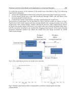
Compare Fig. 5. and Fig. 6. with Fig. 7. and Fig. 8., although the steady states are the same in
these figures, the dynamic responses of them are with much difference, and the objectives
are satisfied as the order appointed before respectively under all the constraints. The reason
of these results is the special initial state:
)0(y
1
is higher than
1
g
(the most important
objective in order [A]:
321
ggg  ), while )0(y
2
is lower than

2
g (the most important
objective in order [B]:
312
ggg 
). So the most important objective of the two orders must
be satisfied with different control input at first respectively. Thus the difference can be seen
from the different decision-making of the choice in control input more obviously: in Fig. 5.
and Fig. 6. the input stays at the lower limit of the constraints at first to meet
1
g
, while in
Fig. 7. and Fig. 8. the input increase as fast as it can to satisfy
2
g at first. The lexicographic
character of LMGA is verified by these comparisons.

0 20 40 60 80 100
20%
40%
60%
80%
Y1
0 20 40 60 80 100
0%
20%
40%
60%
Y2
0 20 40 60 80 100

0%
50%
100%
Time (second)
U

Fig. 5. Control simulation: priority order [A] and p=1
Multi-objective Nonlinear Model Predictive Control: Lexicographic Method 175

With this disposal, the elements in the future sequence of control input
)1pk(u)1k(u)k(u   are not independent as before, and the only unknown
variable here in NMPC is the increment of instant control input
)k(u

, which can determine
all the later control input. The dimension of unknown variable in NMPC now decreases
from
pi
to i remarkably, where i is only the dimension of control input, thus the
computational load is no longer depend on the length of the predictive horizon like many
other MPC (NMPC). So, it is very convenient to use long predictive horizon to obtain better
control quality without additional computational load under this strategy. Because MPC
(NMPC) will repeat the dynamic optimization at every sample time, and only
)1k(u)k(u)k(u

 will be carried out actually in MPC (NMPC), this strategy is surely
efficient here. At last, in stair-like control strategy, it also supposes the future increment of
control input will change in the same direction, which can prevent the frequent oscillation of
control input’s increment, while this kind of oscillation is very harmful to the actuators of
practical control plants. A visible description of this control strategy is shown in Fig. 4.

4.4 Multi-objective NMPC based on GA
Based on the proposed LMGA and PSMGA, the NMPC now can be established directly.
Because NMPC is an online dynamic optimal algorithm, the following steps of NMPC will
be executed repeatedly at every sample time to calculate the instant control input.
Step 1: the LMGA (PSMGA) initialize individuals as different
)k(u (with
population M) under the constraints in (5-3) with historic data
)1k(u

.
Step 2: create M offspring individuals by evolutionary operations as mentioned in
the end of Section 3.1. In control problem, we usually can use real number coding, linear
crossover, stochastic mutation and the lethal penalty in GA for NMPC.
Suppose
21
P,P are
parents and
1 2
,O O are offspring, linear crossover operator 10



and stochastic
mutation operator

is Gaussian white noise with zero mean, the operations can be
described briefly as bellow:

2122
1211
P)1(PO
P)1(PO


,
10



(10)

Step 3: predictions of future outputs (
)k|pk(y
ˆ
)k|2k(y
ˆ
)k|1k(y
ˆ
iii
 
,
i=1,2) are carried out by (5-1) and (5-2) on all the 2M individuals (M parents and M
offspring), and their fitness will be calculated. In this control problem, the fitness function
F

of each objective is transformed from its objective function J easily as follow, to meet the
value demand of ]1,0[F


, in which J is described by (6) or (8):

)1J(1F


(11)

To obtain the robustness to model mismatch, feedback compensation can be used in
prediction, thus the latest predictive errors
2,1i),1k|k(y
ˆ
)k(y)k(e
iii




should be added
into every predictive output
pj1 ,2,11),k|jk(y
ˆ
i

.
Step 4: the M individuals with higher fitness in the 2M individuals will be
remained as new parents.

Step 5: if the condition of ending evaluation is met, the best individual will be the
increment of instant control input
)k(u of NMPC, which is taken into practice by the

actuator. Else, the process should go back to Step 2, to resume dynamic optimization of
NMPC based on LMGA (PSMGA).

4.5 Simulations and analysis of lexicographic multi-objective NMPC
First, the simulation about lexicographic Multi-objective NMPC will be carried out. Choose
control objectives as:
%]60%,40[)k(y:g
11
 , %]40%,20[)k(y:g
22
 , %30y:g
23
 . Consider
the physical character of the system, two different order of priorities can be chosen as: [A]:
321
ggg  , [B]:
312
ggg  , and they will have the same initial state as %80)0(y
1
 ,
%0)0(y
2
 and %20)0(u  . Parameters of NMPC are 85.0,95.0  for both
1
y and
2
y ,
and parameters of GA are 9.0 , while

is a zero mean Gaussian white noise, whose variance

is 5. Since the feasible control input set is relatively small in our problem according to constraints
(5-3), it is enough to have only 10 individuals in our simulation, and they will evolve for 20
generations. While in process control practice, because the sample time is often has a time scale of
minutes, even hours, we can have much more individuals and they can evolve much more
generations to get a satisfactory solution. (In following figures, dash-dot lines denote
21
g,g , dot
line denote
3
g and solid lines denote u,y,y
21
)
Compare Fig. 5. and Fig. 6. with Fig. 7. and Fig. 8., although the steady states are the same in
these figures, the dynamic responses of them are with much difference, and the objectives
are satisfied as the order appointed before respectively under all the constraints. The reason
of these results is the special initial state:
)0(y
1
is higher than
1
g
(the most important
objective in order [A]:
321
ggg  ), while )0(y
2
is lower than
2
g (the most important
objective in order [B]:

312
ggg 
). So the most important objective of the two orders must
be satisfied with different control input at first respectively. Thus the difference can be seen
from the different decision-making of the choice in control input more obviously: in Fig. 5.
and Fig. 6. the input stays at the lower limit of the constraints at first to meet
1
g
, while in
Fig. 7. and Fig. 8. the input increase as fast as it can to satisfy
2
g at first. The lexicographic
character of LMGA is verified by these comparisons.

0 20 40 60 80 100
20%
40%
60%
80%
Y1
0 20 40 60 80 100
0%
20%
40%
60%
Y2
0 20 40 60 80 100
0%
50%
100%

Time (second)
U

Fig. 5. Control simulation: priority order [A] and p=1
Model Predictive Control176

0 20 40 60 80 100
20%
40%
60%
80%
Y1
0 20 40 60 80 100
0%
20%
40%
60%
Y2
0 20 40 60 80 100
0%
50%
100%
U
Time
(
second
)

Fig. 6. Control simulation: priority order [A] and p=20

0 20 40 60 80 100
20%
40%
60%
80%
Y1
0 20 40 60 80 100
0%
20%
40%
60%
Y2
0 20 40 60 80 100
0%
50%
100%
Time (second)
U

Fig. 7. Control simulation: priority order [B] and p=1
0 20 40 60 80 100
20%
40%
60%
80%
Y1
0 20 40 60 80 100
0%
20%
40%

60%
Y2
0 20 40 60 80 100
0%
50%
100%
Time (second)
U

Fig. 8. Control simulation: priority order [B] and p=20

And the difference in control input with different predictive horizon can also be observed
from above figures: the control input is much smoother when the predictive horizon

becomes longer, while the output is similar with the control result of shorter predictive
horizon. It is the common character of NMPC.

0 20 40 60 80 100
40%
60%
80%
100%
Y1
0 20 40 60 80 100
0%
20%
40%
60%
Y2
0 20 40 60 80 100

0%
50%
100%
Time (second)
U

Fig. 9. Control simulation: when an objective cannot be satisfied

In Fig. 9.,
1
g is changed as %]80%,60[y
1

, while other objectives and parameters are kept
the same as those of Fig. 6., so that
3
g can’t be satisfied at steady state. The result shows that
1
y will stay at lower limit of
1
g to reach set-point of
3
g as close as possible, when
1
g must
be satisfied first in order [A]. This result also shows the lexicographic character of LMGA
obviously.

0 20 40 60 80 100
20%

40%
60%
80%
Y1
0 20 40 60 80 100
0%
20%
40%
60%
Y2
0 20 40 60 80 100
0%
50%
100%
Time (second)
U

Fig. 10. Control simulation: when model mismatch

Finally, we would consider about of the model mismatch, here the simulative plant is
changed, by increasing the flux coefficient 0.2232 to 0.25 in (5-1) and (5-2), while all the
objectives, parameters and predictive model are kept the same as those of Fig. 6. The result
in Fig. 10. shows the robustness to model mismatch of the controller with error
compensation in prediction, as mentioned in Section 4.4.

Multi-objective Nonlinear Model Predictive Control: Lexicographic Method 177

0 20 40 60 80 100
20%
40%

60%
80%
Y1
0 20 40 60 80 100
0%
20%
40%
60%
Y2
0 20 40 60 80 100
0%
50%
100%
U
Time
(
second
)

Fig. 6. Control simulation: priority order [A] and p=20

0 20 40 60 80 100
20%
40%
60%
80%
Y1
0 20 40 60 80 100
0%
20%

40%
60%
Y2
0 20 40 60 80 100
0%
50%
100%
Time (second)
U

Fig. 7. Control simulation: priority order [B] and p=1
0 20 40 60 80 100
20%
40%
60%
80%
Y1
0 20 40 60 80 100
0%
20%
40%
60%
Y2
0 20 40 60 80 100
0%
50%
100%
Time (second)
U

Fig. 8. Control simulation: priority order [B] and p=20

And the difference in control input with different predictive horizon can also be observed
from above figures: the control input is much smoother when the predictive horizon

becomes longer, while the output is similar with the control result of shorter predictive
horizon. It is the common character of NMPC.

0 20 40 60 80 100
40%
60%
80%
100%
Y1
0 20 40 60 80 100
0%
20%
40%
60%
Y2
0 20 40 60 80 100
0%
50%
100%
Time (second)
U

Fig. 9. Control simulation: when an objective cannot be satisfied

In Fig. 9.,

1
g is changed as %]80%,60[y
1
 , while other objectives and parameters are kept
the same as those of Fig. 6., so that
3
g can’t be satisfied at steady state. The result shows that
1
y will stay at lower limit of
1
g to reach set-point of
3
g as close as possible, when
1
g must
be satisfied first in order [A]. This result also shows the lexicographic character of LMGA
obviously.

0 20 40 60 80 100
20%
40%
60%
80%
Y1
0 20 40 60 80 100
0%
20%
40%
60%
Y2

0 20 40 60 80 100
0%
50%
100%
Time (second)
U

Fig. 10. Control simulation: when model mismatch

Finally, we would consider about of the model mismatch, here the simulative plant is
changed, by increasing the flux coefficient 0.2232 to 0.25 in (5-1) and (5-2), while all the
objectives, parameters and predictive model are kept the same as those of Fig. 6. The result
in Fig. 10. shows the robustness to model mismatch of the controller with error
compensation in prediction, as mentioned in Section 4.4.

Model Predictive Control178

4.6 Simulations and analysis of partially stratified multi-objective NMPC
To obtain evident comparison to Section 4.5, simulations are carried out with the same
parameters (
85.0,95.0  for both
1
y and
2
y , predictive horizon p=20 and the same
GA parameters), and the only difference is an additional objective on
1
y
in the form of a
setpoint.

The four control objectives now are
%]60%,40[)k(y:g
11
 , %]40%,20[)k(y:g
22
 ,
%30y:g
23
 , %50y:g
14
 , and then choose the new different order of priorities as: [A]:
4321
gggg  , [B]:
4312
gggg  , if we still use lexicographic multi-objective NMPC
as Section 4.5, the control result in Fig. 11. and Fig. 12. is completely the same as Fig. 6. and
Fig. 8., when there are only three objectives
321
ggg ，， . That means, the additional
objective
4
g (setpoint of
1
y ) could not be considered by the controller in both situations
above, because the solution of
3
g (setpoint of
2
y ) is already a single-point set of u . (In
following figures, dash-dot lines denote

21
g,g , dot line denote
43
g,g and solid lines denote
u,y,y
21
)
0 20 40 60 80 100
20%
40%
60%
80%
Y1
0 20 40 60 80 100
0%
20%
40%
60%
Y2
0 20 40 60 80 100
0%
50%
100%
Time
(
second
)
U

Fig. 11. Control simulation: priority order [A] of four objectives, NMPC based on LMGA

0 20 40 60 80 100
20%
40%
60%
80%
Y1
0 20 40 60 80 100
0%
20%
40%
60%
Y2
0 20 40 60 80 100
0%
50%
100%
Time
(
second
)
U

Fig. 12. Control simulation: priority order [B] of four objectives, NMPC based on LMGA

In another word, in lexicographic multi-objective NMPC based on LMGA, if optimization of
an objective uses out all the degree of freedom on control inputs (often an objective in the
form of setpoint), or an objective cannot be completely satisfied (often an objective in the
form of extremum, such as minimization of cost that can not be zero), the objectives with
lower priorities will not be take into account at all. But this is not rational in most practice

cases, for complex process industrial manufacturing, there are often many objectives in the
form of setpoint in a multi-objective control problem, if we handle them with the
lexicographic method, usually, we can only satisfy only one of them. Take the proposed
two-tank system as example,
3
g and
4
g are both in the form of setpoint, seeing about the
steady-state control result in Fig. 13. and Fig. 14., if we want to satisfy
%30y:g
23
 , then
1
y will stay at 51.99%, else if we want to satisfy %50y:g
14

, then
2
y will stay at 28.92%,
the errors of the dissatisfied output are both more than 1%.

100 110 120 130 140 150
30%
40%
50%
60%
70%
Y1
100 110 120 130 140 150
10%

20%
30%
40%
50%
Time (second)
Y2

Fig. 13. Steady-state control result when
3
g is completely satisfied
100 110 120 130 140 150
30%
40%
50%
60%
70%
Y1
100 110 120 130 140 150
10%
20%
30%
40%
50%
Time (second)
Y2

Fig. 14. Steady-state control result when
4
g is completely satisfied

In the above analysis, the mentioned disadvantage comes from the absolute, rigid
management of lexicographic method, if we don’t develop it, NMPC based on LMGA can
only be used in very few control practical problem. Actually, in industrial practice,
objectives in the form of setpoint or extremum are often with lower importance, they are
usually objectives for higher demand on product quality, manufacturing cost and so on,
Multi-objective Nonlinear Model Predictive Control: Lexicographic Method 179

4.6 Simulations and analysis of partially stratified multi-objective NMPC
To obtain evident comparison to Section 4.5, simulations are carried out with the same
parameters (
85.0,95.0


 for both
1
y and
2
y , predictive horizon p=20 and the same
GA parameters), and the only difference is an additional objective on
1
y
in the form of a
setpoint.
The four control objectives now are
%]60%,40[)k(y:g
11
 , %]40%,20[)k(y:g
22
 ,
%30y:g

23
 , %50y:g
14

, and then choose the new different order of priorities as: [A]:
4321
gggg  , [B]:
4312
gggg  , if we still use lexicographic multi-objective NMPC
as Section 4.5, the control result in Fig. 11. and Fig. 12. is completely the same as Fig. 6. and
Fig. 8., when there are only three objectives
321
ggg ，， . That means, the additional
objective
4
g (setpoint of
1
y ) could not be considered by the controller in both situations
above, because the solution of
3
g (setpoint of
2
y ) is already a single-point set of u . (In
following figures, dash-dot lines denote
21
g,g , dot line denote
43
g,g and solid lines denote
u,y,y
21

)
0 20 40 60 80 100
20%
40%
60%
80%
Y1
0 20 40 60 80 100
0%
20%
40%
60%
Y2
0 20 40 60 80 100
0%
50%
100%
Time
(
second
)
U

Fig. 11. Control simulation: priority order [A] of four objectives, NMPC based on LMGA

0 20 40 60 80 100
20%
40%
60%
80%

Y1
0 20 40 60 80 100
0%
20%
40%
60%
Y2
0 20 40 60 80 100
0%
50%
100%
Time
(
second
)
U

Fig. 12. Control simulation: priority order [B] of four objectives, NMPC based on LMGA

In another word, in lexicographic multi-objective NMPC based on LMGA, if optimization of
an objective uses out all the degree of freedom on control inputs (often an objective in the
form of setpoint), or an objective cannot be completely satisfied (often an objective in the
form of extremum, such as minimization of cost that can not be zero), the objectives with
lower priorities will not be take into account at all. But this is not rational in most practice
cases, for complex process industrial manufacturing, there are often many objectives in the
form of setpoint in a multi-objective control problem, if we handle them with the
lexicographic method, usually, we can only satisfy only one of them. Take the proposed
two-tank system as example,
3
g and

4
g are both in the form of setpoint, seeing about the
steady-state control result in Fig. 13. and Fig. 14., if we want to satisfy
%30y:g
23
 , then
1
y will stay at 51.99%, else if we want to satisfy %50y:g
14
 , then
2
y will stay at 28.92%,
the errors of the dissatisfied output are both more than 1%.

100 110 120 130 140 150
30%
40%
50%
60%
70%
Y1
100 110 120 130 140 150
10%
20%
30%
40%
50%
Time (second)
Y2

Fig. 13. Steady-state control result when
3
g is completely satisfied
100 110 120 130 140 150
30%
40%
50%
60%
70%
Y1
100 110 120 130 140 150
10%
20%
30%
40%
50%
Time (second)
Y2

Fig. 14. Steady-state control result when
4
g is completely satisfied

In the above analysis, the mentioned disadvantage comes from the absolute, rigid
management of lexicographic method, if we don’t develop it, NMPC based on LMGA can
only be used in very few control practical problem. Actually, in industrial practice,
objectives in the form of setpoint or extremum are often with lower importance, they are
usually objectives for higher demand on product quality, manufacturing cost and so on,
Model Predictive Control180

which is much less important than the objectives about safety and other basic
manufacturing demand. Especially, for objectives in the form of setpoint, under many kinds
of disturbances, it always can not be accurately satisfied while it is also not necessary to
satisfy them accurately.
A traditional way to improve it is to add slack variables into objectives in the form of setpoint or
extremum. Setpoint may be changed into a narrow range around it, and instead of an extremum,
the satisfaction of a certain threshold value will be required. For example, in the two-tank
system’s control problem, setpoint
%30y:g
23
 could be redefined as %1%30y:g
23
 .
Another way is modified LMGA into PSMGA as mentioned in Section 3, because sometimes
there is no need to divide these objectives with into different priorities respectively, and they are
indeed parallel. Take order [A] for example, we now can reform the multi-objective control
problem of the two-tank system as:
443321321
ggggGGG  . Choose weight
coefficients as
1,30
43
 and other parameters the same as those of Fig. 6., while NMPC
base on PSMGA has the similar dynamic state control result to that of NMPC based on LMGA,
the steady state control result is evidently developed as in Fig. 15. and Fig. 16.,
1
y
stays at
50.70% and
2

y stays at 29.27%, both of them are in the 0.8% neighborhood of setpoint in
43
g,g .
0 20 40 60 80 100
20%
40%
60%
80%
Y1
0 20 40 60 80 100
0%
20%
40%
60%
Y2
0 20 40 60 80 100
0%
50%
100%
Time
(
second
)
U

Fig. 15. NMPC based on PSMGA: priority order [A]

100 110 120 130 140 150
30%
40%

50%
60%
70%
Y1
100 110 120 130 140 150
10%
20%
30%
40%
50%
Time (second)
Y2

Fig. 16. Steady-state control result of NMPC base on PSMGA

4.7 Some discussions
In the above simulative examples, there is only one control input, but for many practical
systems, coordinated control of multi-input is also a serious problem. The brief discussions
on multi-input proposed NMPC can be achieved if we still use priorities for inputs. If all the
inputs have the same priority, in another word, it is no obvious difference among them in
economic cost or other factors, we can just increase the dimension of GA’s individual. But,
in many cases, the inputs actually also have different priorities: for certain output, different
input often has different gain on it with different economic cost. The cheap ones with large
gain are always preferred by manufacturers. In this case, we can form anther priority list,
and then inputs will be used to solve the control problem one by one, using single input
NMPC as the example in Section 4, that can divide an MIMO control problem into some
SIMO control problems.
We should point out that, the two kinds of stratified structures proposed in this paper are
basic structures for multi-objective controllers, though we use NMPC to realize them in this
chapter, they are independent with control algorithms indeed. For certain multi-objective

control problem, other proper controllers and computational method can be used.
Another point must be mentioned is that, NMPC proposed in this paper is based on LMGA
and PSMGA, because it is hard for most NMPC to get an online analytic solution. But the
LMGA and PSMGA are also suitable for other control algorithms, the only task is to modify
the fitness function, by introducing the information from the control algorithm which will
be used.
At last, all the above simulations could been done in 40-200ms by PC (with 2.7 GHz CPU,
2.0G Memory and programmed by Matlab 6.5), which is much less than the sample time of
the system (1 second), that means controllers proposed in this chapter are actually
applicable online.

5. Conclusion
In this chapter, to avoid the disadvantages of weight coefficients in multi-objective dynamic
optimization, lexicographic (completely stratified) and partially stratified frameworks of
multi-objective controller are proposed. The lexicographic framework is absolutely priority-
driven and the partially stratified framework is a modification of it, they both can solve the
multi-objective control problem with the concept of priority for objective’s relative
importance, while the latter one is more flexible, without the rigidity of lexicographic
method.
Then, nonlinear model predictive controllers based on these frameworks are realized based
on the modified genetic algorithm, in which a series of dynamic coefficients is introduced to
construct the combined fitness function. With stair–like control strategy, the online
computational load is reduced and the performance is developed. The simulative study of a
two-tank system indicates the efficiency of the proposed controllers and some deeper
discussions are given briefly at last.
The work of this chapter is supported by Fund for Excellent Post Doctoral Fellows (K. C.
Wong Education Foundation, Hong Kong, China and Chinese Academy of Sciences),
Science and Technological Fund of Anhui Province for Outstanding Youth (08040106910),
and the authors also thank for the constructive advices from Dr. De-Feng HE, College of
Information Engineering, Zhejiang University of Technology, China.

Multi-objective Nonlinear Model Predictive Control: Lexicographic Method 181

which is much less important than the objectives about safety and other basic
manufacturing demand. Especially, for objectives in the form of setpoint, under many kinds
of disturbances, it always can not be accurately satisfied while it is also not necessary to
satisfy them accurately.
A traditional way to improve it is to add slack variables into objectives in the form of setpoint or
extremum. Setpoint may be changed into a narrow range around it, and instead of an extremum,
the satisfaction of a certain threshold value will be required. For example, in the two-tank
system’s control problem, setpoint
%30y:g
23

could be redefined as %1%30y:g
23


.
Another way is modified LMGA into PSMGA as mentioned in Section 3, because sometimes
there is no need to divide these objectives with into different priorities respectively, and they are
indeed parallel. Take order [A] for example, we now can reform the multi-objective control
problem of the two-tank system as:
443321321
ggggGGG  . Choose weight
coefficients as
1,30
43




 and other parameters the same as those of Fig. 6., while NMPC
base on PSMGA has the similar dynamic state control result to that of NMPC based on LMGA,
the steady state control result is evidently developed as in Fig. 15. and Fig. 16.,
1
y
stays at
50.70% and
2
y stays at 29.27%, both of them are in the 0.8% neighborhood of setpoint in
43
g,g .
0 20 40 60 80 100
20%
40%
60%
80%
Y1
0 20 40 60 80 100
0%
20%
40%
60%
Y2
0 20 40 60 80 100
0%
50%
100%
Time
(
second

)
U

Fig. 15. NMPC based on PSMGA: priority order [A]

100 110 120 130 140 150
30%
40%
50%
60%
70%
Y1
100 110 120 130 140 150
10%
20%
30%
40%
50%
Time (second)
Y2

Fig. 16. Steady-state control result of NMPC base on PSMGA

4.7 Some discussions
In the above simulative examples, there is only one control input, but for many practical
systems, coordinated control of multi-input is also a serious problem. The brief discussions
on multi-input proposed NMPC can be achieved if we still use priorities for inputs. If all the
inputs have the same priority, in another word, it is no obvious difference among them in
economic cost or other factors, we can just increase the dimension of GA’s individual. But,
in many cases, the inputs actually also have different priorities: for certain output, different

input often has different gain on it with different economic cost. The cheap ones with large
gain are always preferred by manufacturers. In this case, we can form anther priority list,
and then inputs will be used to solve the control problem one by one, using single input
NMPC as the example in Section 4, that can divide an MIMO control problem into some
SIMO control problems.
We should point out that, the two kinds of stratified structures proposed in this paper are
basic structures for multi-objective controllers, though we use NMPC to realize them in this
chapter, they are independent with control algorithms indeed. For certain multi-objective
control problem, other proper controllers and computational method can be used.
Another point must be mentioned is that, NMPC proposed in this paper is based on LMGA
and PSMGA, because it is hard for most NMPC to get an online analytic solution. But the
LMGA and PSMGA are also suitable for other control algorithms, the only task is to modify
the fitness function, by introducing the information from the control algorithm which will
be used.
At last, all the above simulations could been done in 40-200ms by PC (with 2.7 GHz CPU,
2.0G Memory and programmed by Matlab 6.5), which is much less than the sample time of
the system (1 second), that means controllers proposed in this chapter are actually
applicable online.

5. Conclusion
In this chapter, to avoid the disadvantages of weight coefficients in multi-objective dynamic
optimization, lexicographic (completely stratified) and partially stratified frameworks of
multi-objective controller are proposed. The lexicographic framework is absolutely priority-
driven and the partially stratified framework is a modification of it, they both can solve the
multi-objective control problem with the concept of priority for objective’s relative
importance, while the latter one is more flexible, without the rigidity of lexicographic
method.
Then, nonlinear model predictive controllers based on these frameworks are realized based
on the modified genetic algorithm, in which a series of dynamic coefficients is introduced to
construct the combined fitness function. With stair–like control strategy, the online

computational load is reduced and the performance is developed. The simulative study of a
two-tank system indicates the efficiency of the proposed controllers and some deeper
discussions are given briefly at last.
The work of this chapter is supported by Fund for Excellent Post Doctoral Fellows (K. C.
Wong Education Foundation, Hong Kong, China and Chinese Academy of Sciences),
Science and Technological Fund of Anhui Province for Outstanding Youth (08040106910),
and the authors also thank for the constructive advices from Dr. De-Feng HE, College of
Information Engineering, Zhejiang University of Technology, China.
Model Predictive Control182

6. References
Alessio A. & Bemporad A. (2009). A survey on explicit model predictive control. Lecture
Notes in Control and Information Sciences (Nonlinear Model Predictive Control:
Towards New Challenging Applications), Vol. 384, pp 345-369, ISSN
0170-8643.
Cannon M. (2004). Efficient nonlinear model predictive control algorithms. Annual Reviews
in Control. Vol.28, No.2, pp229-237, ISSN
1367-5788.
Coello C. A. C. (2000). An Updated Survey of GA-Based Multiobjective Optimization
Techniques, ACM Computing Surveys, Vol.32, No.2, pp109-143, ISSN 0360-0300.
Meadowcroft T. A.; Stephanopoulos G. & Brosilow C. (1992). The modular multivariable
controller: I: steady-state properties. AIChE Journal, Vol.38, No.8, pp1254-1278,
ISSN 0001-1541.
Ocampo-Martinez C.; Ingimundarson A.; Vicenç P. & J. Quevedo. (2008). Objective
prioritization using lexicographic minimizers for MPC of sewer networks. IEEE
Transactions on Control Systems Technology, Vol. 16, No.1, pp113-121, ISSN 1063-
6536.
Wu G.; Lu X. D.; Ying A. G.; Xue M. S.; Zhang Z. G. & Sun D. M. (2000). Modular
Multivariable Self-tuning Regulator. Acta Automatica Sinica, Vol.26, No.6, pp811-
815, ISSN 0254-4156.

Yuzgec U.; Becerikli Y. & Turker M. (2006). Nonlinear Predictive Control of a Drying Process
Using Genetic Algorithms, ISA Transactions, Vol.45, No.4, pp589-602, ISSN 0019-
0578.
Zheng T.; Wu G.; He D. F.; Yue D. Z. (2008). An Efficient Model Nonlinear Predictive
Control Algorithm Based on Stair-like Control Strategy, Proceedings of the 27
th

Chinese Control Conference, Vol.3, pp557-561, ISBN 9787811243901, Kunming,
China, July, 2008, Beihang University Press, Beijing, China.
Model Predictive Trajectory Control for High-Speed Rack Feeders 183
Model Predictive Trajectory Control for High-Speed Rack Feeders
Harald Aschemann and Dominik Schindele
0
Model Predictive Trajectory Control
for High-Speed Rack Feeders
Harald Aschemann and Dominik Schindele
Chair of Mechatronics, University of Rostock
18059 Rostock, Germany
1. Introduction
Rack feeders represent the commonly used handling systems for the automated operation of
high-bay rackings. To further increase the handling capacity by shorter transport times, con-
trol measures are necessary for the reduction of excited structural oscillations, see also Asche-
mann & Ritzke (2009). One possible approach is given by flatness-based feedforward control,
where the desired control inputs are determined by dynamic system inversion using the de-
sired trajectories for the flat outputs as in Bachmayer et al. (2008) and M. Bachmayer & Ulbrich
(2008). However, both publications consider only a constant mass position in vertical direc-
tion on an elastic beam without any feedback control. A variational approach is presented in
Kostin & Saurin (2006) to compute an optimal feedforward control for an elastic beam. Unfor-
tunately, feedforward control alone is not sufficient to guarantee small tracking errors when
model uncertainty is present or disturbances act on the system. For this reason in this con-

tribution a model predictive control (MPC) design is presented for fast trajectory control. In
general, at model predictive control the optimal input vector is mostly calculated by minimis-
ing a quadratic cost function as, e.g., in Wang & Boyd (2010) or Magni & Scattolini (2004). In
contrast, the here considered MPC approach aims at reducing future state errors, see Jung &
Wen (2004), and allows for a relatively small computational effort as required in a real-time
implementation. Hence, the proposed MPC algorithm is well suited for systems with fast
dynamics, e.g., a high-speed linear axis with pneumatic muscles as presented in Schindele &
Aschemann (2008) or high-speed rack feeders as in the given case. A further attractive char-
acteristic of this MPC approach is its applicability to linear as well as nonlinear systems.
For the experimental investigation of modern control approaches to active oscillation damp-
ing as well as tracking control, a test rig of a high-speed rack feeder has been build up at the
Chair of Mechatronics at the University of Rostock, see Figure 1. The experimental set-up
consists of a carriage driven by an electric DC servo motor via a toothed belt, on which an
elastic beam as the vertical supporting structure is mounted. On this beam structure, a cage
with variable load mass is guided relocatably in vertical direction. This cage with the coor-
dinate y
K
(t) in horizontal direction and x
K
(t) in vertical direction represents the tool center
point (TCP) of the rack feeder that should track desired trajectories as accurate as possible.
The movable cage is driven by a tooth belt and an electric DC servo motor as well. The angles
of the actuators are measured by internal angular transducers, respectively. Additionally, the
horizontal position of the carriage is detected by a magnetostrictive transducer. Both axes are
operated with a fast underlying velocity control on the current converter. Consequently, the
8
Model Predictive Control184
Fig. 1. Experimental set-up of the high-speed rack feeder (left) and the corresponding elastic
multibody model (right).
corresponding velocities deal as new control input, and the implementational effort is tremen-

dously reduced as compared to the commonly used force or torque input, like in Staudecker
et al. (2008), where passivity techniques were employed for feedback control of a similar set-
up. Two strain gauges are used to determine the bending deformation of the elastic beam.
Basis of the control design for the rack feeder is a planar elastic multibody system, where
for the mathematical description of the bending deflection of the elastic beam a Ritz ansatz
is introduced, covering for instance the first bending mode. The decentralised feedforward
and feedback control design for both axes is performed employing a linearised state space
representation, respectively. Given couplings between both axes are taken into account by the
gain-scheduling technique with the normalised vertical cage position as scheduling param-
eter, see also Aschemann & Ritzke (2010). This leads to an adaptation of the whole control
structure for the horizontal axis. The capability of the proposed control concept is shown by
experimental results from the test set-up with regard to tracking behaviour and damping of
bending oscillations. Especially the artificial damping introduced by the closed control loop
represents a main improvement. The maximum velocity of the TCP during the tracking ex-
periments is approx. 2.5 m/s.
2. Control-oriented modelling of the mechatronic system
Elastic multibody models have proven advantageously for the control-oriented modelling of
flexible mechanical systems. For the feedforward and feedback control design of the rack
feeder a multibody model with three rigid bodies - the carriage (mass m
S
), the cage movable
on the beam structure (mass m
K
, mass moment of inertia θ
K
), and the end mass at the tip of
the beam (mass m
E
) - and an elastic Bernoulli beam (density ρ, cross sectional area A, Youngs
modulus E, second moment of area I

zB
, and length ) is chosen. The varying vertical position
x
K
(t) of the cage on the beam is denoted by the dimensionless system parameter
κ
(
t
)
=
x
κ
(
t
)
l
. (1)
The elastic degrees of freedom of the beam concerning the bending deflection can be described
by the following Ritz ansatz
v
(
x, t
)
=
¯
¯
v
1
(
x

)
v
1
(
t
)
=

3
2

x
l

2
−
1
2

x
l

3

v
1
(
t
)
, (2)

which takes into account only the first bending mode. The vector of generalised coordinates
results in
q
(
t
)
=

y
S
(
t
)
v
1
(
t
)

. (3)
The nonlinear equations of motion can be derived either by Lagrange’s equations or, advan-
tageously, by the Newton-Euler approach, cf. Shabana (2005). After a linearisation for small
bending deflections, the equations of motion can be stated in M-D-K form
M ¨q
(
t
)
+
D ˙q
(

t
)
+
Kq
(
t
)
=
h ·
[
F
SM
(
t
)
−
F
SR
(
˙
y
S
(
t
))]
. (4)
The symmetric mass matrix is given by
M
=


m
S
+ ρAl + m
K
+ m
E
3
8
ρAl +
m
K
κ
2
2
[
3 − κ
]
+
m
E
3
8
ρAl +
m
K
κ
2
2
[
3 − κ

]
+
m
E
m
22

, (5)
with m
22
=
33
140
ρAl +
6ρI
zB
5l
+
m
K
κ
2
4
[
3 − κ
]
2
+
9θ
K

κ
2
l
2

1
− κ +
κ
2
4

+ m
E
. The damping matrix,
which is specified with stiffness-proportional damping properties, and the stiffness matrix
become
D
=

0 0
0
3k
d
EI
zB
l
3

, (6)
K

=

0 0
0
3EI
zB
l
3
−
3
8
ρAg −
3m
K
gκ
3
l

1
+
3κ
2
20
−
3κ
4

−
6m
E

g
5l

. (7)
The input vector of the generalised forces, which accounts for the control input as well as the
disturbance input, reads
h
=

1 0

T
. (8)
The electric drive for the carriage is operated with a fast underlying velocity control on the
current converter. The resulting dynamic behaviour is characterised by a first-order lag system
with a time constant T
1y
T
1y
¨
y
S
(
t
)
+
˙
y
S
(

t
)
=
v
S
(
t
)
. (9)
This differential equation replaces now the equation of motion for the carriage in the mechan-
ical system model, which leads to a modified mass matrix as well as a modified damping
matrix
M
y
=

T
1y
0
3
8
ρAl +
m
K
κ
2
2
[
3 − κ
]

+
m
E
m
22

, (10)
Model Predictive Trajectory Control for High-Speed Rack Feeders 185
Fig. 1. Experimental set-up of the high-speed rack feeder (left) and the corresponding elastic
multibody model (right).
corresponding velocities deal as new control input, and the implementational effort is tremen-
dously reduced as compared to the commonly used force or torque input, like in Staudecker
et al. (2008), where passivity techniques were employed for feedback control of a similar set-
up. Two strain gauges are used to determine the bending deformation of the elastic beam.
Basis of the control design for the rack feeder is a planar elastic multibody system, where
for the mathematical description of the bending deflection of the elastic beam a Ritz ansatz
is introduced, covering for instance the first bending mode. The decentralised feedforward
and feedback control design for both axes is performed employing a linearised state space
representation, respectively. Given couplings between both axes are taken into account by the
gain-scheduling technique with the normalised vertical cage position as scheduling param-
eter, see also Aschemann & Ritzke (2010). This leads to an adaptation of the whole control
structure for the horizontal axis. The capability of the proposed control concept is shown by
experimental results from the test set-up with regard to tracking behaviour and damping of
bending oscillations. Especially the artificial damping introduced by the closed control loop
represents a main improvement. The maximum velocity of the TCP during the tracking ex-
periments is approx. 2.5 m/s.
2. Control-oriented modelling of the mechatronic system
Elastic multibody models have proven advantageously for the control-oriented modelling of
flexible mechanical systems. For the feedforward and feedback control design of the rack
feeder a multibody model with three rigid bodies - the carriage (mass m

S
), the cage movable
on the beam structure (mass m
K
, mass moment of inertia θ
K
), and the end mass at the tip of
the beam (mass m
E
) - and an elastic Bernoulli beam (density ρ, cross sectional area A, Youngs
modulus E, second moment of area I
zB
, and length ) is chosen. The varying vertical position
x
K
(t) of the cage on the beam is denoted by the dimensionless system parameter
κ
(
t
)
=
x
κ
(
t
)
l
. (1)
The elastic degrees of freedom of the beam concerning the bending deflection can be described
by the following Ritz ansatz

v
(
x, t
)
=
¯
¯
v
1
(
x
)
v
1
(
t
)
=

3
2

x
l

2
−
1
2


x
l

3

v
1
(
t
)
, (2)
which takes into account only the first bending mode. The vector of generalised coordinates
results in
q
(
t
)
=

y
S
(
t
)
v
1
(
t
)


. (3)
The nonlinear equations of motion can be derived either by Lagrange’s equations or, advan-
tageously, by the Newton-Euler approach, cf. Shabana (2005). After a linearisation for small
bending deflections, the equations of motion can be stated in M-D-K form
M ¨q
(
t
)
+
D ˙q
(
t
)
+
Kq
(
t
)
=
h ·
[
F
SM
(
t
)
−
F
SR
(

˙
y
S
(
t
))]
. (4)
The symmetric mass matrix is given by
M
=

m
S
+ ρAl + m
K
+ m
E
3
8
ρAl +
m
K
κ
2
2
[
3 − κ
]
+
m

E
3
8
ρAl +
m
K
κ
2
2
[
3 − κ
]
+
m
E
m
22

, (5)
with m
22
=
33
140
ρAl +
6ρI
zB
5l
+
m

K
κ
2
4
[
3 − κ
]
2
+
9θ
K
κ
2
l
2

1
− κ +
κ
2
4

+ m
E
. The damping matrix,
which is specified with stiffness-proportional damping properties, and the stiffness matrix
become
D
=


0 0
0
3k
d
EI
zB
l
3

, (6)
K
=

0 0
0
3EI
zB
l
3
−
3
8
ρAg −
3m
K
gκ
3
l

1

+
3κ
2
20
−
3κ
4

−
6m
E
g
5l

. (7)
The input vector of the generalised forces, which accounts for the control input as well as the
disturbance input, reads
h
=

1 0

T
. (8)
The electric drive for the carriage is operated with a fast underlying velocity control on the
current converter. The resulting dynamic behaviour is characterised by a first-order lag system
with a time constant T
1y
T
1y

¨
y
S
(
t
)
+
˙
y
S
(
t
)
=
v
S
(
t
)
. (9)
This differential equation replaces now the equation of motion for the carriage in the mechan-
ical system model, which leads to a modified mass matrix as well as a modified damping
matrix
M
y
=

T
1y
0

3
8
ρAl +
m
K
κ
2
2
[
3 − κ
]
+
m
E
m
22

, (10)
Model Predictive Control186
D
y
=

1 0
0
3k
d
EI
zB
l

3

. (11)
The stiffness matrix K
= K
y
and the input vector for the generalised forces h = h
y
, however,
remain unchanged. Hence, the equations of motion are given by
¨q
= −M
−1
y
K
y
q − M
−1
y
D
y
˙q + M
−1
y
h
y
v
S
. (12)
For control design, the system representation is reformulated in state space form

˙x
y
=

˙q
¨q

=

0 I
−M
−1
y
K
y
−M
−1
y
D
y


 
A
y

q
˙q



 
x
y
+

0
M
−1
y
h
y


 
b
y
v
S

u
y
. (13)
The design model for the vertical movement of the cage can be directly stated in state space
representation. Here, an underlying velocity control is employed on the current converter,
which is also described by a first-order lag system
T
1x
¨
x
K

(
t
)
+
˙
x
K
(
t
)
=
v
K
(
t
)
. (14)
The corresponding state space description follows immediately in the form
˙x
x
=

˙
x
K
¨
x
K

=


0 1
0
−
1
T
1x


 
A
x

x
K
˙
x
K


 
x
x
+

0
1
T
1x



 
b
x
v
K

u
x
. (15)
Whereas the state space respresentation for the horizontal y-axis depends on the varying sys-
tem parameter κ
(t), the description of the x-axis is invariant. A gain-scheduling, hence, is
necessary only for the horizontal axis in y-direction.
3. Decentralised control design
As for control, a decentralised approach is followed, at which the coupling of the vertical
cage motion with the horizontal axis is taken into account by gain-scheduling techniques. For
the control of the cage position x
K
(t) a simple proportional feedback in combination with
feedforward control, which is based on the inverse transfer function of this axis, is sufficient
v
K
(
t
)
=
K
R
(

x
Kd
(
t
)
−
x
K
(
t
))
+
˙
x
Kd
(
t
)
+
T
1x
¨
x
Kd
(
t
)
. (16)
For this purpose, the desired trajectory x
Kd

(t) and its first two time derivatives are available
from trajectory planning. The design of the state feedback for the horizontal motion is carried
out by the MPC approach, which is explained in the following chapter.
Hight-Speed Rack Feeder
Vertical Axis
[
y
S
˙
y
S
]
[

d
˙

d
¨

d
]
Gain-Scheduled
Model
Predictive
Control
v
S
t 
v

K
t 
w
y
=
[
y
Kd
˙
y
Kd
¨
y
Kd

y
Kd
y
4
Kd
]
Inverse
Kinematics
[
v
1
˙
v
1
]

Real
Differentiation
Real
Differentiation
Feedforward
Control
Proportional
Feedback
x
K
t 
[
y
Sd
˙
y
Sd
v
1d
˙
v
1d
]
Horizontal Axis
Inverse
Dynamics
v
Sd
w
x

=
[
x
Kd
˙
x
Kd
¨
x
Kd
]
Normalisation

d
Fig. 2. Implementation of the control structure.
4. Model Predictive Control
The main idea of the control approach consists in a minimisation of a future tracking error
in terms of the predicted state vector based on the actual state and the desired state vector
resulting from trajectory planning, see Lizarralde et al. (1999), Jung & Wen (2004). The min-
imisation is achieved by repeated approximate numerical optimisation in each time step, in
the given case using the Newton-Raphson technique. The optimisation is initialised in each
time step with the optimisation result of the preceding time step in form of the input vector.
The MPC-algorithm is based on the following discrete-time state space representation
x
k+1
= Ax
k
+ bu
k
, (17)

y
k
= c
T
x
k
, (18)
with the state vector x
k
∈ R
n
, the control input u
k
∈ R and the output vector y
k
∈ R.
The constant M specifies the prediction horizon T
P
as a multiple of the sampling time t
s
, i.e.
T
P
= M · t
s
. The predicted input vector at time k becomes
u
k,M
=


u
(k)
1
, , u
(k)
M

T
, (19)
Model Predictive Trajectory Control for High-Speed Rack Feeders 187
D
y
=

1 0
0
3k
d
EI
zB
l
3

. (11)
The stiffness matrix K
= K
y
and the input vector for the generalised forces h = h
y
, however,

remain unchanged. Hence, the equations of motion are given by
¨q
= −M
−1
y
K
y
q − M
−1
y
D
y
˙q + M
−1
y
h
y
v
S
. (12)
For control design, the system representation is reformulated in state space form
˙x
y
=

˙q
¨q

=


0 I
−M
−1
y
K
y
−M
−1
y
D
y

  
A
y

q
˙q

  
x
y
+

0
M
−1
y
h
y


  
b
y
v
S

u
y
. (13)
The design model for the vertical movement of the cage can be directly stated in state space
representation. Here, an underlying velocity control is employed on the current converter,
which is also described by a first-order lag system
T
1x
¨
x
K
(
t
)
+
˙
x
K
(
t
)
=
v

K
(
t
)
. (14)
The corresponding state space description follows immediately in the form
˙x
x
=

˙
x
K
¨
x
K

=

0 1
0
−
1
T
1x

  
A
x


x
K
˙
x
K

  
x
x
+

0
1
T
1x

  
b
x
v
K

u
x
. (15)
Whereas the state space respresentation for the horizontal y-axis depends on the varying sys-
tem parameter κ
(t), the description of the x-axis is invariant. A gain-scheduling, hence, is
necessary only for the horizontal axis in y-direction.
3. Decentralised control design

As for control, a decentralised approach is followed, at which the coupling of the vertical
cage motion with the horizontal axis is taken into account by gain-scheduling techniques. For
the control of the cage position x
K
(t) a simple proportional feedback in combination with
feedforward control, which is based on the inverse transfer function of this axis, is sufficient
v
K
(
t
)
=
K
R
(
x
Kd
(
t
)
−
x
K
(
t
))
+
˙
x
Kd

(
t
)
+
T
1x
¨
x
Kd
(
t
)
. (16)
For this purpose, the desired trajectory x
Kd
(t) and its first two time derivatives are available
from trajectory planning. The design of the state feedback for the horizontal motion is carried
out by the MPC approach, which is explained in the following chapter.
Hight-Speed Rack Feeder
Vertical Axis
[
y
S
˙
y
S
]
[

d

˙

d
¨

d
]
Gain-Scheduled
Model
Predictive
Control
v
S
t 
v
K
t 
w
y
=
[
y
Kd
˙
y
Kd
¨
y
Kd


y
Kd
y
4
Kd
]
Inverse
Kinematics
[
v
1
˙
v
1
]
Real
Differentiation
Real
Differentiation
Feedforward
Control
Proportional
Feedback
x
K
t 
[
y
Sd
˙

y
Sd
v
1d
˙
v
1d
]
Horizontal Axis
Inverse
Dynamics
v
Sd
w
x
=
[
x
Kd
˙
x
Kd
¨
x
Kd
]
Normalisation

d
Fig. 2. Implementation of the control structure.

4. Model Predictive Control
The main idea of the control approach consists in a minimisation of a future tracking error
in terms of the predicted state vector based on the actual state and the desired state vector
resulting from trajectory planning, see Lizarralde et al. (1999), Jung & Wen (2004). The min-
imisation is achieved by repeated approximate numerical optimisation in each time step, in
the given case using the Newton-Raphson technique. The optimisation is initialised in each
time step with the optimisation result of the preceding time step in form of the input vector.
The MPC-algorithm is based on the following discrete-time state space representation
x
k+1
= Ax
k
+ bu
k
, (17)
y
k
= c
T
x
k
, (18)
with the state vector x
k
∈ R
n
, the control input u
k
∈ R and the output vector y
k

∈ R.
The constant M specifies the prediction horizon T
P
as a multiple of the sampling time t
s
, i.e.
T
P
= M · t
s
. The predicted input vector at time k becomes
u
k,M
=

u
(k)
1
, , u
(k)
M

T
, (19)
Model Predictive Control188
with u
k,M
∈ R
M
. The predicted state vector at the end of the prediction horizon φ

M
(x
k
, u
k,M
)
is obtained by repeated substitution of k by k + 1 in the discrete-time state equation (17)
x
k+2
= Ax
k+1
+ bu
k+1
= A
2
x
k
+ Abu
k
+ bu
k+1
.
.
.
x
k+M
= A
M
x
k

+ A
M−1
bu
k
+ A
M−2
bu
k−1
+ . . . + bu
k+M−1
= φ
M
(x
k
, u
k,M
) .
(20)
The difference of φ
M
(x
k
, u
k,M
) and the desired state vector x
d
yields the final control error
e
M,k
= φ

M
(x
k
, u
k,M
) − x
d
, (21)
i.e. to the control error at the end of the prediction horizon. The cost function to be minimised
follows as
J
MPC
=
1
2
· e
T
M,k
e
M,k
, (22)
and, hence, the necessary condition for an extremum can be stated as
∂J
MPC
∂e
M,k
= e
M,k
!
= 0 . (23)

A Taylor-series expansion of (23) at u
k,M
in the neighbourhood of the optimal solution leads
to the following system of equations
0
= e
M,k
+
∂φ
M
∂u
k,M
∆u
k,M
+ T.h.O (24)
The vector ∆u
k,M
denotes the difference which has to be added to the input vector u
k,M
to
obtain the optimal solution. The n equations (24) represent an under-determined set of equa-
tions with m
· M unknowns having an infinite number of solutions. An unique solution for
∆u
k,M
can be determined by solving the following L
2
-optimisation problem with (24) as side
condition
J

=
1
2
· ∆ u
T
k,M
∆u
k,M
+ λ
T

e
M,k
+
∂φ
M
∂u
k,M
∆u
k,M

. (25)
Consequently, the necessary conditions can be stated as
∂J
∂∆u
k,M
!
= 0 = ∆u
k,M
+


∂φ
M
∂u
k,M

T
λ,
∂J
∂λ
!
= 0 = e
M,k
+
∂φ
M
∂u
k,M
∆u
k,M
,
(26)
which results in e
M,k
e
M,k
=
∂φ
M
∂u

k,M

∂φ
M
u
k,M

T
  
S
(
φ
M
,u
k,M
)
λ . (27)
If the matrix S

φ
M
, u
k,M

is invertible, the vector λ can be calculated as follows
λ
= S
−1

φ

M
, u
k,M

e
M,k
. (28)
An almost singular matrix S

φ
M
, u
k,M

can be treated by a modification of (28)
λ
=

µI
+ S

φ
M
, u
k,M

−1
e
M,k
, (29)

where I denotes the unity matrix. The regularisation parameter µ
> 0 in (29) may be chosen
constant or may be calculated by a sophisticated algorithm. The latter solution improves
the convergence of the optimisation but increases, however, the computational complexity.
Solving (26) for ∆u
k,M
and inserting λ according to (28) or (29), directly yields the L
2
-optimal
solution
∆u
k,M
= −

∂φ
M
∂u
k,M

T
S
−1

φ
M
, u
k,M

e
M,k

= −

∂φ
M
∂u
k,M

†
e
M,k
.
(30)
Here,

∂φ
M
∂u
k,M

†
denotes the Moore-Penrose pseudo inverse of
∂φ
M
∂u
k,M
. The overall MPC-
algorithm can be described as follows:
Choice of the initial input vector u
0,M
at time k = 0, e.g. u

0,M
= 0, and repetition of steps a) -
c) at each sampling time k
≥ 0:
a) Calculation of an improved input vector v
k,M
according to
v
k,M
= u
k,M
− η
k

∂φ
M
∂u
k,M

†
e
M,k
. (31)
The step width η
k
can be determined with, e.g., the Armijo-rule.
b) For the calculation of u
k+1,M
the elements of the vector v
k,M

have to be shifted by one
element and the steady-state input u
d
corresponding to the final state has to be inserted
at the end
u
k+1,M
=

0
((M−1)×1)
1

u
d
+

0
((M−1)×1)
I
(M−1)
0 0
(1×(M−1))

v
k,M
. (32)
In general, the steady-state control input u
d
can be computed from

x
d
= Ax
d
+ bu
d
. (33)
Alternatively, the desired input vector u
d
can be calculated by an inverse system model.
If the system is differentially flat, see Fliess et al. (1995) the desired input u
d
can be cal-
culated exactly by the flat system output and a finite number of its time derivative. For
non-flat outputs -as in the given case- the approach presented in chapter 4.4 is useful.
c) The first element of the improved input vector v
k,M
is applied as control input at time k
u
k
=

1 0
(1×(M−1))

v
k,M
. (34)
In the proposed algorithm only one iteration is performed per time step. A similar approach
using several iteration steps is described in Weidemann et al. (2004). An improvement of

the trajectory tracking behaviour can be achieved if an input vector resulting from an inverse
system model is used as initial vector for the subsequent optimisation step instead of the last
input vector. The slightly modified algorithm can be stated as follows
Model Predictive Trajectory Control for High-Speed Rack Feeders 189
with u
k,M
∈ R
M
. The predicted state vector at the end of the prediction horizon φ
M
(x
k
, u
k,M
)
is obtained by repeated substitution of k by k + 1 in the discrete-time state equation (17)
x
k+2
= Ax
k+1
+ bu
k+1
= A
2
x
k
+ Abu
k
+ bu
k+1

.
.
.
x
k+M
= A
M
x
k
+ A
M−1
bu
k
+ A
M−2
bu
k−1
+ . . . + bu
k+M−1
= φ
M
(x
k
, u
k,M
) .
(20)
The difference of φ
M
(x

k
, u
k,M
) and the desired state vector x
d
yields the final control error
e
M,k
= φ
M
(x
k
, u
k,M
) − x
d
, (21)
i.e. to the control error at the end of the prediction horizon. The cost function to be minimised
follows as
J
MPC
=
1
2
· e
T
M,k
e
M,k
, (22)

and, hence, the necessary condition for an extremum can be stated as
∂J
MPC
∂e
M,k
= e
M,k
!
= 0 . (23)
A Taylor-series expansion of (23) at u
k,M
in the neighbourhood of the optimal solution leads
to the following system of equations
0
= e
M,k
+
∂φ
M
∂u
k,M
∆u
k,M
+ T.h.O (24)
The vector ∆u
k,M
denotes the difference which has to be added to the input vector u
k,M
to
obtain the optimal solution. The n equations (24) represent an under-determined set of equa-

tions with m
· M unknowns having an infinite number of solutions. An unique solution for
∆u
k,M
can be determined by solving the following L
2
-optimisation problem with (24) as side
condition
J
=
1
2
· ∆ u
T
k,M
∆u
k,M
+ λ
T

e
M,k
+
∂φ
M
∂u
k,M
∆u
k,M


. (25)
Consequently, the necessary conditions can be stated as
∂J
∂∆u
k,M
!
= 0 = ∆u
k,M
+

∂φ
M
∂u
k,M

T
λ,
∂J
∂λ
!
= 0 = e
M,k
+
∂φ
M
∂u
k,M
∆u
k,M
,

(26)
which results in e
M,k
e
M,k
=
∂φ
M
∂u
k,M

∂φ
M
u
k,M

T
  
S
(
φ
M
,u
k,M
)
λ . (27)
If the matrix S

φ
M

, u
k,M

is invertible, the vector
λ can be calculated as follows
λ
= S
−1

φ
M
, u
k,M

e
M,k
. (28)
An almost singular matrix S

φ
M
, u
k,M

can be treated by a modification of (28)
λ
=

µI
+ S


φ
M
, u
k,M

−1
e
M,k
, (29)
where I denotes the unity matrix. The regularisation parameter µ
> 0 in (29) may be chosen
constant or may be calculated by a sophisticated algorithm. The latter solution improves
the convergence of the optimisation but increases, however, the computational complexity.
Solving (26) for ∆u
k,M
and inserting λ according to (28) or (29), directly yields the L
2
-optimal
solution
∆u
k,M
= −

∂φ
M
∂u
k,M

T

S
−1

φ
M
, u
k,M

e
M,k
= −

∂φ
M
∂u
k,M

†
e
M,k
.
(30)
Here,

∂φ
M
∂u
k,M

†

denotes the Moore-Penrose pseudo inverse of
∂φ
M
∂u
k,M
. The overall MPC-
algorithm can be described as follows:
Choice of the initial input vector u
0,M
at time k = 0, e.g. u
0,M
= 0, and repetition of steps a) -
c) at each sampling time k
≥ 0:
a) Calculation of an improved input vector v
k,M
according to
v
k,M
= u
k,M
− η
k

∂φ
M
∂u
k,M

†

e
M,k
. (31)
The step width η
k
can be determined with, e.g., the Armijo-rule.
b) For the calculation of u
k+1,M
the elements of the vector v
k,M
have to be shifted by one
element and the steady-state input u
d
corresponding to the final state has to be inserted
at the end
u
k+1,M
=

0
((M−1)×1)
1

u
d
+

0
((M−1)×1)
I

(M−1)
0 0
(1×(M−1))

v
k,M
. (32)
In general, the steady-state control input u
d
can be computed from
x
d
= Ax
d
+ bu
d
. (33)
Alternatively, the desired input vector u
d
can be calculated by an inverse system model.
If the system is differentially flat, see Fliess et al. (1995) the desired input u
d
can be cal-
culated exactly by the flat system output and a finite number of its time derivative. For
non-flat outputs -as in the given case- the approach presented in chapter 4.4 is useful.
c) The first element of the improved input vector v
k,M
is applied as control input at time k
u
k

=

1 0
(1×(M−1))

v
k,M
. (34)
In the proposed algorithm only one iteration is performed per time step. A similar approach
using several iteration steps is described in Weidemann et al. (2004). An improvement of
the trajectory tracking behaviour can be achieved if an input vector resulting from an inverse
system model is used as initial vector for the subsequent optimisation step instead of the last
input vector. The slightly modified algorithm can be stated as follows
Model Predictive Control190
a) Calculation of the ideal input vector u
(d)
k,M
by evaluating an inverse system model with
the specified reference trajectory as well as a certain number β
∈ N of its time deriva-
tives
u
(d)
k,M
= u
(d)
k,M

y
d

, ˙y
d
, ,
(β)
y
d

. (35)
b) Calculation of the improved input vector v
k,M
based on the equation
v
k,M
= u
(d)
k,M
− η
k

∂φ
M
∂u
k,M

†
e
M,k
. (36)
c) Application of the first element of v
k,M

to the process
u
k
=

1 0
(1×(M−1))

v
k,M
. (37)
If the reference trajectory is known in advance, the according reference input vector u
(d)
k,M
can
be computed offline. Consequently, the online computational time remains unaffected.
4.1 Numerical calculations
The analytical computation of the Jacobian
∂φ
M
∂u
k,M
becomes increasingly complex for larger
values of M. Therefore, a numerical approach is preferred taking advantage of the chain rule
with i
= 0, , M − 1
∂φ
M
∂u
(k)

i+1
=
∂φ
M
∂x
k+M−1
·
∂x
k+M−1
∂x
k+M−2
· . . . ·
∂x
k+i+2
∂x
k+i+1
·
∂x
k+i+1
∂u
(k)
i+1
.
(38)
In this way, the Jacobian can be computed as follows
∂φ
M
∂u
k,M
= [A

M−1
b, A
M−2
b, , Ab, b] . (39)
For the inversion of the symmetric and positive definite matrix S

φ
M
, u
k,M

=
∂φ
M
∂u
k,M

∂φ
M
∂u
k,M

T
the Cholesky-decomposition has proved advantageous in terms of compu-
tational effort.
4.2 Choice of the MPC design parameters
The most important MPC design parameter is the prediction horizon T
P
, which is given as the
product of the sampling time t

s
and the constant value M. Large values of T
P
lead to a slow
and smooth transient behaviour and result in a robust and stable control loop. For fast trajec-
tory tracking, however, a smaller value T
P
is desirable concerning a small tracking error. The
choice of the sampling time t
s
is crucial as well: a small sampling time is necessary regard-
ing both discretisation error and stability; however, the MPC-algorithm has to be evaluated
in real-time within the sampling inverval. Furthermore, the smaller t
s
, the larger becomes M
for a given prediction horizon, which in turn increases the computational complexity of the
optimisation step. Consequently, a system-specific trade-off has to be made for the choice of
M and t
s
. This paper follows the moving horizon approach with a constant prediction hori-
zon and, hence, a constant dimension m
· M of the corresponding optimisation problem in
constrast to the shrinking horizon approach according to Weidemann et al. (2004).
T
P
e
M,0
x
0
φ

M
(x , u )
0
0,M
Desired Trajectory
x
t
t
s
φ
M
(x , u )
1
1,M
x
1
e
M,1
t
s
M
Predicted State
x
d,0
x
d,1
Fig. 3. Design parameters.
4.3 Input constraints
One major advantage of predictive control is the possibility to easily account for input con-
straints, which are present in almost all control applications. To this end, the cost function can

be extended with a corresponding term
h
(u
(k)
j
) =







0 u
min
≤ u
(k)
j
≤ u
max
g
1
(u
(k)
j
) for u
(k)
j
> u
max

g
2
(u
(k)
j
) u
(k)
j
< u
min
, (40)
which has to be evaluated componentwise, i.e. for each input variable at each sampling time.
Thus, the contribution of the additional input constraints depending on u
k,M
is given by
z
(u
k,M
) =
M
∑
j=1
h(u
(k)
j
). (41)
Instead of e
M,k
, the extended vector


e
T
M,k
, z

T
has to be minimised in the MPC-algorithm.
4.4 MPC of the horizontal cage position
The state space representation for the cage position control in y-direction design is given by
(13). The discrete-time representation of the continous-time system is obtained by Euler dis-
cretisation
x
y,k+1
=

I
+ t
s
· A
y
(
κ
)

x
y,k
+ t
s
· b
y

(
κ
)
u
y,k
. (42)
Model Predictive Trajectory Control for High-Speed Rack Feeders 191
a) Calculation of the ideal input vector u
(d)
k,M
by evaluating an inverse system model with
the specified reference trajectory as well as a certain number β
∈ N of its time deriva-
tives
u
(d)
k,M
= u
(d)
k,M

y
d
, ˙y
d
, ,
(β)
y
d


. (35)
b) Calculation of the improved input vector v
k,M
based on the equation
v
k,M
= u
(d)
k,M
− η
k

∂φ
M
∂u
k,M

†
e
M,k
. (36)
c) Application of the first element of v
k,M
to the process
u
k
=

1 0
(1×(M−1))


v
k,M
. (37)
If the reference trajectory is known in advance, the according reference input vector u
(d)
k,M
can
be computed offline. Consequently, the online computational time remains unaffected.
4.1 Numerical calculations
The analytical computation of the Jacobian
∂φ
M
∂u
k,M
becomes increasingly complex for larger
values of M. Therefore, a numerical approach is preferred taking advantage of the chain rule
with i
= 0, , M − 1
∂φ
M
∂u
(k)
i+1
=
∂φ
M
∂x
k+M−1
·

∂x
k+M−1
∂x
k+M−2
· . . . ·
∂x
k+i+2
∂x
k+i+1
·
∂x
k+i+1
∂u
(k)
i+1
.
(38)
In this way, the Jacobian can be computed as follows
∂φ
M
∂u
k,M
= [A
M−1
b, A
M−2
b, , Ab, b] . (39)
For the inversion of the symmetric and positive definite matrix S

φ

M
, u
k,M

=
∂φ
M
∂u
k,M

∂φ
M
∂u
k,M

T
the Cholesky-decomposition has proved advantageous in terms of compu-
tational effort.
4.2 Choice of the MPC design parameters
The most important MPC design parameter is the prediction horizon T
P
, which is given as the
product of the sampling time t
s
and the constant value M. Large values of T
P
lead to a slow
and smooth transient behaviour and result in a robust and stable control loop. For fast trajec-
tory tracking, however, a smaller value T
P

is desirable concerning a small tracking error. The
choice of the sampling time t
s
is crucial as well: a small sampling time is necessary regard-
ing both discretisation error and stability; however, the MPC-algorithm has to be evaluated
in real-time within the sampling inverval. Furthermore, the smaller t
s
, the larger becomes M
for a given prediction horizon, which in turn increases the computational complexity of the
optimisation step. Consequently, a system-specific trade-off has to be made for the choice of
M and t
s
. This paper follows the moving horizon approach with a constant prediction hori-
zon and, hence, a constant dimension m
· M of the corresponding optimisation problem in
constrast to the shrinking horizon approach according to Weidemann et al. (2004).
T
P
e
M,0
x
0
φ
M
(x , u )
0
0,M
Desired Trajectory
x
t

t
s
φ
M
(x , u )
1
1,M
x
1
e
M,1
t
s
M
Predicted State
x
d,0
x
d,1
Fig. 3. Design parameters.
4.3 Input constraints
One major advantage of predictive control is the possibility to easily account for input con-
straints, which are present in almost all control applications. To this end, the cost function can
be extended with a corresponding term
h
(u
(k)
j
) =








0 u
min
≤ u
(k)
j
≤ u
max
g
1
(u
(k)
j
) for u
(k)
j
> u
max
g
2
(u
(k)
j
) u
(k)

j
< u
min
, (40)
which has to be evaluated componentwise, i.e. for each input variable at each sampling time.
Thus, the contribution of the additional input constraints depending on u
k,M
is given by
z
(u
k,M
) =
M
∑
j=1
h(u
(k)
j
). (41)
Instead of e
M,k
, the extended vector

e
T
M,k
, z

T
has to be minimised in the MPC-algorithm.

4.4 MPC of the horizontal cage position
The state space representation for the cage position control in y-direction design is given by
(13). The discrete-time representation of the continous-time system is obtained by Euler dis-
cretisation
x
y,k+1
=

I
+ t
s
· A
y
(
κ
)

x
y,k
+ t
s
· b
y
(
κ
)
u
y,k
. (42)
Model Predictive Control192

Using this simple discretisation method, the computational effort for the MPC-algorithm can
be kept acceptable. By the way, no significant improvement could be obtained for the given
system with the Heun discretisation method because of the small sampling time t
s
= 3 ms.
Only in the case of large sampling times, e.g. t
s
> 20 ms, the increased computational effort
caused by a sophisticated time discretisation method is advantageous. Then, the smaller dis-
cretisation error allows for less time integration steps for a specified prediction horizon, i.e. a
smaller number M. As a result, the smaller number of time steps can overcompensate the
larger effort necessary for a single time step.
The ideal input u
d
(t) can be obtained in continous time as function of the output variable
y
K
(t) = c
T
y
x
y
(t) =

1
1
2
κ
2
(

3 − κ
)
0 0

x
y
(t) , (43)
and a certain number of its time derivatives. For this purpose the corresponding transfer
function of the system under consideration is employed
Y
K
(
s
)
U
d
(
s
)
=
c
T
y

sI
− A
y

−1
b

y
=

b
0
+ b
1
· s + b
2
· s
2

N
(
s
)
. (44)
Obviously, the numerator of the control transfer function contains a second degree polynomial
in s, leading to two transfer zeros. This shows that the considered output y
K
(t) represents a
non-flat output variable that makes computing of the feedforward term more difficult. A pos-
sible way for calculating the desired input variable is given by a modification of the numerator
of the control transfer function by introducing a polynomial ansatz for the feedforward action
according to
U
d
(
s
)

=

k
V0
+ k
V1
· s + . . . + k
V4
· s
4

Y
Kd
(
s
)
. (45)
For its realisation the desired trajectory y
Kd
(t) as well as the first four time derivatives are
available from a trajectory planning module. The feedforward gains can be computed from
a comparison of the corresponding coefficients in the numerator as well as the denominator
polynomials of
Y
K
(
s
)
Y
Kd

(
s
)
=

b
0
+ . . . + b
2
· s
2

k
V0
+ . . . + k
V4
· s
4

N
(
s
)
=
b
V0

k
Vj


+ b
V1

k
Vj

· s + . . . + b
V6

k
Vj

· s
6
a
0
+ a
1
· s + . . . + s
4
(46)
according to
a
i
= b
Vi

k
Vj


, i
= 0, . . . , n = 4 . (47)
This leads to parameter-dependent feedforward gains k
Vj
= k
Vj
(κ). It is obvious that due
the higher numerator degree in the modified control transfer function a remaining dynamics
must be accepted. Lastly, the desired input variable in the time domain is represented by
u
d
(t) = u
d

˙
y
Kd
(t),
¨
y
Kd
(t),

y
Kd
(t), y
(4)
Kd
(t), κ


. (48)
To obtain the desired system states as function of the output trajectory the output equation
0 5 10 15
0
0.2
0.4
0.6
0.8
t in s
y
K
in m
0 5 10 15
−2
−1
0
1
2
t in s
y
Kpd
in m/s
0 5 10 15
0
0.2
0.4
0.6
0.8
t in s
x

K
in m
0 5 10 15
−1.5
−1
−0.5
0
0.5
1
1.5
t in s
x
Kpd
in m/s
y
Kd
y
K
x
Kd
x
K
Fig. 4. Desired trajectories for the cage motion: desired and actual position in horizontal
direction (upper left corner), desired and actual position in vertical direction (upper right
corner), actual velocity in horizontal direction (lower left corner) and actual velocity in vertical
direction (lower right corner).
and its first three time derivatives are considered. Including the equations of motion (12)
yields the following set of equations
y
Kd

(t) = y
S
(t) +
1
2
κ
2
(
3 − κ
)
·
v
1
(t), (49)
˙
y
Kd
(t) =
˙
y
S
(t) +
1
2
κ
2
(
3 − κ
)
·

˙
v
1
(t), (50)
¨
y
Kd
(t) =
¨
y
S
(t) +
1
2
κ
2
(
3 − κ
)
·
¨
v
1
(t) =
¨
y
K
(
v
1

(t),
˙
y
S
(t),
˙
v
1
(t), u
d
(t), κ
)
, (51)

y
Kd
(t) =

y
K
(
v
1
(t),
˙
y
S
(t),
˙
v

1
(t), u
d
(t),
˙
u
d
(t), κ
)
. (52)
Solving equation (49) to (52) for the system states results in the desired state vector
x
d
(t) =




y
Sd
(
y
Kd
(t),
˙
y
Kd
(t),
¨
y

Kd
(t),

y
Kd
(t), u
d
(t),
˙
u
d
(t), κ
)
v
1d
(
˙
y
Kd
(t),
¨
y
Kd
(t),

y
Kd
(t), u
d
(t),

˙
u
d
(t), κ
)
˙
y
Sd
(
˙
y
Kd
(t),
¨
y
Kd
(t),

y
Kd
(t), u
d
(t),
˙
u
d
(t), κ
)
˙
v

1d
(
˙
y
Kd
(t),
¨
y
Kd
(t),

y
Kd
(t), u
d
(t),
˙
u
d
(t), κ
)




. (53)
This equation still contains the inverse dynamics u
d
(t) and its time derivative
˙

u
d
. Substituting
u
d
for equation (48) and
˙
u
d
(t) for the time derivative of (48), which can be calculated analyti-