Advances in Solid-State Lasers: Development and Applicationsduration and in the end limits Part 12 pptx
Bạn đang xem bản rút gọn của tài liệu. Xem và tải ngay bản đầy đủ của tài liệu tại đây (7.55 MB, 40 trang )
Advances in Solid-State Lasers: Development and Applications
432
where S1 and S2 are, respectively, the distances G1–P2 and P3–G2. For S < 2p, G1 is imaged
behind G2 and the resulting GDD is positive. For S > 2p, G1 is imaged before G2 and the
resulting GDD is negative. The three cases are illustrated in Fig. 17.
The chirp of the pulse can be varied by changing S = S1 + S2. It is simpler to keep S1
constant and to finely adjust S2 for changing the GDD. The variation of S2 is performed by
mounting G2 on a linear translator and moving it along an axis coincident with the straight
line that connects G2 to P3. Since the beam diffracted from G2 is collimated in a constant
direction, the radiation reflected from P4 is focused always on the same output point.
Therefore, the compressor has no moving parts except the translation of G2 for the fine
tuning of the GDD.
The modeling of the compressor is done by ray-tracing simulations. The group delay is
calculated for different values of the distance S. The GDD is then defined as the derivative of
the group delay with respect to the frequency. The higher effects on the phase of the pulse
can be analogously calculated by successive derivatives.
Fig. 17. Operation of the XUV attosecond compressor: a) GDD equal to zero; b) positive
GDD; c) negative GDD.
As a test case of the optical configuration, the design of a compressor in the 12-24 nm region
is presented. The grazing angle on the mirrors is chosen to be 3° for high reflectivity. The
acceptance angle is 6 mrad, which matches the divergence of XUV ultrashort pulses. The
size of the illuminated portion of the paraboloidal mirrors results 23 mm
× 1.2 mm. On such
S”
G2≡G1’
S2
S3
Intermediate
Plane
S
(a) GDD = 0
P1 P2
P3
G1
S’
λc
P4
P3
S’
λc
P4
S”
G2
(b) GDD > 0
G1’
P3
S’
λc
P4
S”
G2
(c) GDD < 0
G1’
Diffraction Gratings for the Selection of Ultrashort Pulses in the Extreme-Ultraviolet
433
a small area, manufacturers routinely can produce paraboloidal mirrors with very-high
quality finishing, both in terms of figuring errors (
λ/30 at 500 nm) and of slope errors (less
than 2
μrad rms). Since the gratings are ruled on plane substrates, the surface finishing is
even better than on curved surfaces. Such precision on the optical surfaces is essential to
have time-delay compensation in the range of tens of attoseconds. The altitude and blaze
angles of the gratings have been selected to optimize the time-delay compensation.
Particular attention must be given to isolate the compressor optics from environmental
vibrations and to precisely align the components in order to realize correct implementation
of the optimal geometry.
The global efficiency of such a compressor can be predicted to be in the 0.10–0.20 range, on
the basis of the efficiency measurements made on the existing off-plane monochromator and
already discussed.
The time-delay compensation of the compressor has been analyzed with ray-tracing
simulations. Once the grating groove density is selected, the time-delay compensation
depends on the choice of altitude and azimuth angles. Both these parameters have to be
optimized in order to minimize the residual spreads of the optical paths. In the case
presented here, the choice of 200 gr/mm groove density, 1.5° altitude, and 4.3° azimuth
gives a residual spread of less than 10 as FWHM in the whole 12-24 nm spectral region. The
characteristics of the compressor are resumed in Tab. 5.
Pulse spectral interval
12-24 nm
Mirrors Off-axis paraboloidal
Input/output arms 200 mm
Acceptance angle
6 mrad
× 6 mrad
Grazing angle
3
°
Size of illuminated area
23 mm
× 1.2 mm
Gratings Plane
Groove density 200 gr/mm
Altitude angle
1.5
°
Blaze angle
4.5
°
Distances
S > 400 mm for negative GDD
Table 5. Parameters of the compressor for the 12-24 nm region.
The calculated results of the compressor’s phase properties are shown in Fig. 18. For S > 400
mm, the GDD is always negative as predicted and the values reported are in agreement
with what is required to compress the pulse as resulting from the HH generation modeling.
An example of compression of a pulse with a positive GDD, modeled according to the
results obtained using the polarization gating technique (Sola et al., 2006; Sansone et al.,
2006), is presented in Fig. 19. Note the clear time compression to a nearly single-cycle pulse.
The scheme of the compressor is very versatile: it can be designed with high throughput in
any spectral interval within the 4-60 nm XUV region. By a simple linear translation of a
single grating, the instrument introduces a variable group delay in the range of few
hundreds attoseconds with constant throughput and either negative or positive group-delay
dispersion. The extended spectral range of operation and the versatility in the control of the
Advances in Solid-State Lasers: Development and Applications
434
group delay allows the compression of XUV attosecond pulses beyond the limitations of the
schemes based on metallic filters.
Fig. 18. Phase properties of the compressor with the parameters listed in Tab. 5: group delay
(top) and group-delay dispersion (GDD).
Fig. 19. Simulation of the compression of a chirped XUV pulse at the output of the
compressor with the parameters listed in Tab. 5. Input pulse parameters: central energy 73
eV (17 nm), bandwidth 25 eV (6 nm), positive chirp with GDD = 5100 as
2
. Compressor: S =
410 mm. FWHM durations: input 350 as, output 75 as.
Diffraction Gratings for the Selection of Ultrashort Pulses in the Extreme-Ultraviolet
435
7. Conclusions
The use of diffraction gratings to perform the spectral selection of ultrashort pulses in the
XUV spectral region has been discussed. The main applications of such technique are the
spectral selection of high-order laser harmonics and free-electron-laser pulses in the
femtosecond time scale.
The realization of monochromators tunable in a broad spectral band in the XUV requires the
use of gratings at grazing incidence. Obviously, the preservation of the time duration of the
pulse at the output of the monochromator is crucial to have both high temporal resolution
and high peak power. A single grating gives a temporal broadening of the ultrafast pulse
because of the diffraction. This effect is negligible for picosecond or longer pulses, but is
dramatic in the femtosecond time scale. Nevertheless, it is possible to design grating
monochromators that do not alter the temporal duration of the pulse in the femtosecond
time scale by using two gratings in a time-delay compensated configuration. In such a
configuration, the second grating compensates for the time and spectral spread introduced
by the first one.
Therefore, the grating monochromators for ultrafast pulses are divided in two main families:
1. the single-grating configuration, that gives intrinsically a temporal broadening of the
ultrafast pulse, but is simple and has high efficiency since it requires the use of one
grating only;
2. the time-delay compensated configuration with two gratings, that has a much shorter
temporal response, in the femtosecond or even shorter time scale, but is more complex
and has a lower efficiency.
Once the experimental requirements are given, aim of the optical design is to select the
configuration that gives the best trade-off between time response and efficiency.
The efficiency is obviously the major factor discriminating among different designs: an
instrument with low efficiency could be not useful for scientific experiments. An innovative
configuration to realize monochromators with high efficiency and broad tunability has been
discussed. It adopts gratings in the off-plane mount, in which the incident light direction
belongs to a plane parallel to the direction of the grooves. The off-plane mount has
efficiency higher than the classical mount and, once the grating groove density has been
selected, it gives minimum temporal response at grazing incidence.
Both single- and double-grating monochromators in the off-plane mount can be designed. In
particular, we have presented in details two applications to the selection of high-order
harmonics, one using a single-grating design and one in a time-delay compensated
configuration. In the latter case, the XUV temporal response at the output of the
monochromator has been measured to be as short as few femtoseconds, confirming the
temporal compensation given by the double-grating design.
Finally, the problem of temporal compression of broadband XUV attosecond pulses by
means of a double-grating compressor has been addressed. The time-delay compensated
design in the off-plane configuration has been modified to realize an XUV attosecond
compressor that can introduce a variable group-delay dispersion to compensate for the
intrinsic chirp of the attosecond pulse.
This class of instruments plays an important role for the photon handling and conditioning
of future ultrashort sources.
Advances in Solid-State Lasers: Development and Applications
436
8. Acknowledgment
The authors would like to remember the essential contribution of Mr. Paolo Zambolin (1965-
2005) to the mechanical design of the time-delay compensated monochromator at LUXOR
(Padova, Italy). The experiments on the beamline ARTEMIS at Rutherford Appleton
Laboratory (UK) are carried on under the management of Dr. Emma Springate and Dr.
Edmund Turcu. The experiments with high-order harmonics at Politecnico Milano (Italy)
are carried on under the management of Prof. Mauro Nisoli and Dr. Giuseppe Sansone.
9. References
Akhmanov, S. A.; Vysloukh, V. A. & Chirkin, A. S. (1992) Optics of Femtosecond Laser Pulses,
American IOP, New York
Cash, W. (1982). Echelle spectrographs at grazing incidence, Appl. Opt. Vol. 21, pp. 710–717
Corkum, P.B. & Krausz, F. (2007). Attosecond science. Nat. Phys. Vol. 3, pp. 381-387
Chiudi Diels, J C.; Rudolph, W. (2006). Ultrashort Laser Pulse Phenomena, Academic Press
Inc., Oxford
Frassetto, F.; Bonora, S.; Villoresi, P.; Poletto, L.; Springate, E.; Froud, C.A.; Turcu, I.C.E.;
Langley, A.J.; Wolff, D.S.; Collier, J.L.; Dhesi, S.S. & Cavalleri, A. (2008). Design and
characterization of the XUV monochromator for ultrashort pulses at the ARTEMIS
facility, Proc. SPIE Vol. 7077, Advances in X-Ray/EUV Optics and Components III,
no. 707713, S. Diego (USA), August 2008, SPIE Publ., Bellingham
Frassetto, F.; Villoresi, P. & Poletto, L. (2008). Optical concept of a compressor for XUV
pulses in the attosecond domain, Opt. Exp. Vol. 16, pp. 6652-6667
Kienberger, R. & Krausz, F. (2004). Subfemtosecond XUV Pulses: Attosecond Metrology and
Spectroscopy, in Few-cycle laser pulse generation and its applications, F.X. Kärtner ed.,
pp. 143-179, Springer, Berlin
Kienberger, R.; Goulielmakis, E.; Uberacker, M.; Baltuska, A.; Yakovlev, V.; Bammer, F.;
Scrinzi, A.; Westerwalbesloh, T.; Kleineberg, U.; Heinzmann, U.; Drescher, M. &
Krausz, F. (2004). Atomic transient recorder, Nature Vol. 427, pp. 817-822
Jaegle', P. (2006). Coherent Sources of XUV Radiation, Springer, Berlin
Lopez-Martens, R.; Varju, K.; Johnsson, P.; Mauritsson, J.; Mairesse, Y.; Salières, P.; Gaarde,
M.B.; Schafer, K.J.; Persson, A.; Svanberg, S.; Wahlström, C G. & L’Huillier, A.
(2005). Amplitude and phase control of attosecond light pulses, Phys. Rev. Lett. Vol.
94, no. 033001
Marciak-Kozlowska, J. (2009). From Femto-to Attoscience and Beyond, Nova Science Publishers
Inc., New York
Patel, N. (2002). Shorter, Brighter, Better. Nature Vol. 415, pp. 110-11
Petit, R. (1980). Electromagnetic theory of gratings, Springer, Berlin
Pascolini, M.; Bonora, S.; Giglia, A.; Mahne, N.; Nannarone, S. & Poletto, L. (2006) Gratings
in the conical diffraction mounting for an EUV time-delay compensated
monochromator, Appl. Opt. Vol. 45, pp. 3253-3562
Paul, P.M.; Toma, E.S.; Breger, P.; Mullot, G.; Auge, F.; Balcou, P.; Muller, H.G. & Agostini,
P. (2001). Observation of a train of attosecond pulses from high harmonic
generation, Science Vol. 292, pp. 1689–1692
Diffraction Gratings for the Selection of Ultrashort Pulses in the Extreme-Ultraviolet
437
Poletto, L. & Tondello, G. (2001). Time-compensated EUV and soft X-ray monochromator for
ultrashort high-order harmonic pulses, Pure Appl. Opt. Vol. 3, pp. 374-379
Poletto, L.; Bonora, S.; Pascolini, M.; Borgatti, F.; Doyle, B.; Giglia, A.; Mahne, N.; Pedio, M.
& Nannarone, S. (2004). Efficiency of gratings in the conical diffraction mounting
for an EUV time-compensated monochromator, Proc. SPIE Vol. 5534, Fourth
Generation X-Ray Sources and Optics II, pp. 144–153, Denver (USA), August 2004,
SPIE Publ., Bellingham
Poletto, L. (2004). Time-compensated grazing-incidence monochromator for extreme-
ultraviolet and soft X-ray high-order harmonics, Appl. Phys. B Vol. 78,
pp. 1013-1016
Poletto, L. & Villoresi, P. (2006). Time-compensated monochromator in the off-plane mount
for extreme-ultraviolet ultrashort pulses, Appl. Opt. Vol. 45, pp. 8577-8585
Poletto, L.; Villoresi, P.; Benedetti, E.; Ferrari, F.; Stagira, S.; Sansone, G.; Nisoli, M. (2007).
Intense femtosecond extreme ultraviolet pulses by using a time-delay compensated
monochromator, Opt. Lett. Vol. 32, pp. 2897-2899
Poletto, L.; Villoresi, P.; Benedetti, E.; Ferrari, F.; Stagira, S.; Sansone, G.; Nisoli, M. (2008).
Temporal characterization of a time-compensated monochromator for high-
efficiency selection of XUV pulses generated by high-order harmonics, J. Opt. Soc.
Am. B Vol. 25, pp. B44-B49
Poletto, L.; Frassetto, F. & Villoresi, P. (2008). Design of an Extreme-Ultraviolet Attosecond
Compressor, J. Opt. Soc. Am. B Vol. 25, pp. B133-B136
Poletto, L. (2009). Tolerances of time-delay compensated monochromators for extreme-
ultraviolet ultrashort pulses, Appl. Opt. Vol. 48, pp. 4526-4535
Saldin, E.L.; Schneidmiller, E.A. & Yurkov, M.V. (2000). The Physics of Free Electron Lasers,
Springer, Berlin
Sansone, G.; Vozzi, C.; Stagira, S. & Nisoli, M. (2004). Nonadiabatic quantum path analysis
of high-order harmonic generation: role of the carrier-envelope phase on short and
long paths, Phys. Rev. A Vol. 70, no. 013411
Sansone, G.; Benedetti, E.; Calegari, F.; Vozzi, C.; Avaldi, L.; Flammini, R.; Poletto, L.;
Villoresi, P.; Altucci, C.; Velotta, R.; Stagira, S.; De Silvestri, S. & Nisoli, M. (2006).
Isolated single-cycle attosecond pulses, Science Vol. 314, pp. 443–446
Sola, J.; Mevel, E.; Elouga, L.; Constant, E.; Strelkov, V.; Poletto, L.; Villoresi, P.; Benedetti, E.;
Caumes, J P.; Stagira, S.; Vozzi, C.; Sansone, G. & Nisoli, M. (2006). Controlling
attosecond electron dynamics by phase-stabilized polarization gating, Nat. Phys.
Vol. 2, pp. 319–322
Villoresi, P. (1999). Compensation of optical path lengths in extreme-ultraviolet and soft-x-
ray monochromators for ultrafast pulses, Appl. Opt. Vol. 38, pp. 6040-6049
Walmsley, I.; Waxer, L. & Dorrer, C. (2001). The role of dispersion in ultrafast optics, Rev.
Sci. Instr. Vol. 72, pp. 1–28
Werner, W. (1977). X-ray efficiencies of blazed gratings in extreme off-plane mountings,
Appl. Opt. Vol. 16, pp. 2078–2080
Werner, W. & Visser, H. (1981). X-ray monochromator designs based on extreme off-plane
grating mountings, Appl. Opt. Vol. 20, pp. 487-492
Wiedemann, H. (2005). Synchrotron Radiation, Springer, Berlin
Advances in Solid-State Lasers: Development and Applications
438
Wieland, M.; Frueke, R.; Wilhein, T.; Spielmann, C.; Pohl, M. & Kleinenberg, U. (2002)
Submicron extreme ultraviolet imaging using high-harmonic radiation, Appl. Phys.
Lett. Vol. 81, pp. 2520-2522
19
High-Harmonic Generation
Kenichi L. Ishikawa
Photon Science Center, Graduate School of Engineering, University of Tokyo
Japan
1. Introduction
We present theoretical aspects of high-harmonic generation (HHG) in this chapter.
Harmonic generation is a nonlinear optical process in which the frequency of laser light is
converted into its integer multiples. Harmonics of very high orders are generated from
atoms and molecules exposed to intense (usually near-infrared) laser fields. Surprisingly,
the spectrum from this process, high-harmonic generation, consists of a plateau where the
harmonic intensity is nearly constant over many orders and a sharp cutoff (see Fig. 5).
The maximal harmonic photon energy E
c
is given by the cutoff law (Krause et al., 1992),
=3.17,
cp p
EI U
+
(1)
where I
p
is the ionization potential of the target atom, and U
p
[eV] =
22
00
/4E
ω
= 9.337 × 10
−14
I
[W/cm
2
] (
λ
[μm])
2
the ponderomotive energy, with E
0
, I and
λ
being the strength, intensity
and wavelength of the driving field, respectively. HHG has now been established as one of
the best methods to produce ultrashort coherent light covering a wavelength range from the
vacuum ultraviolet to the soft x-ray region. The development of HHG has opened new
research areas such as attosecond science and nonlinear optics in the extreme ultraviolet
(xuv) region.
Rather than by the perturbation theory found in standard textbooks of quantum mechanics,
many features of HHG can be intuitively and even quantitatively explained in terms of
electron rescattering trajectories which represent the semiclassical three-step model and the
quantum-mechanical Lewenstein model. Remarkably, various predictions of the three-step
model are supported by more elaborate direct solution of the time-dependent Schrödinger
equation (TDSE). In this chapter, we describe these models of HHG (the three-step model,
the Lewenstein model, and the TDSE).
Subsequently, we present the control of the intensity and emission timing of high harmonics
by the addition of xuv pulses and its application for isolated attosecond pulse generation.
2. Model of high-harmonic generation
2.1 Three Step Model (TSM)
Many features of HHG can be intuitively and even quantitatively explained by the
semiclassical three-step model (Fig. 1)(Krause et al., 1992; Schafer et al., 1993; Corkum, 1993).
According to this model, in the first step, an electron is lifted to the continuum at the nuclear
position with no kinetic energy through tunneling ionization (ionization). In the second step,
Advances in Solid-State Lasers: Development and Applications
440
the subsequent motion is governed classically by an oscillating electric field (propagation). In
the third step, when the electron comes back to the nuclear position, occasionally, a
harmonic, whose photon energy is equal to the sum of the electron kinetic energy and the
ionization potential I
p
, is emitted upon recombination. In this model, although the quantum
mechanics is inherent in the ionization and recombination, the propagation is treated
classically.
Fig. 1. Three step model of high-harmonic generation.
Let us consider that the laser electric field E(t), linearly polarized in the z direction, is given
by
00
()= cos ,Et E t
ω
(2)
where E
0
and
ω
0
denotes the field amplitude and frequency, respectively. If the electron is
ejected at t = t
i
, by solving the equation of motion for the electron position z(t) with the
initial conditions
()=0,
i
zt (3)
()=0,
i
zt
(4)
we obtain,
()()
0
00000
2
0
( ) = cos cos sin .
iii
E
zt t t t t t
ωωωωω
ω
⎡
−+− ⎤
⎣
⎦
(5)
It is convenient to introduce the phase
θ
≡
ω
0
t. Then Equation 5 is rewritten as,
()()
0
2
0
( ) = cos cos sin ,
iii
E
z
θ
θθθθθ
ω
⎡
−+− ⎤
⎣
⎦
(6)
and we also obtain, for the kinetic energy E
kin
,
()
2
()=2 sin sin .
kin p i
EU
θθθ
− (7)
One obtains the time (phase) of recombination t
r
(
θ
r
) as the roots of the equation z(t) = 0 (z(
θ
)
= 0). Then the energy of the photon emitted upon recombination is given by E
kin
(
θ
r
) + I
p
.
High-Harmonic Generation
441
Figure 2 shows E
kin
(
θ
r
)/U
p
as a function of phase of ionization
θ
i
and recombination
θ
r
for 0 <
θ
i
<
π
. The electron can be recombined only if 0 <
θ
i
<
π
/2; it flies away and never returns to
the nuclear position if
π
/2 <
θ
i
<
π
. E
kin
(
θ
r
) takes the maximum value 3.17U
p
at
θ
i
= 17° and
θ
r
= 255°. This beautifully explains why the highest harmonic energy (cutoff) is given by
3.17U
p
+ I
p
. It should be noted that at the time of ionization the laser field, plotted in thin
solid line, is close to its maximum, for which the tunneling ionization probability is high.
Thus, harmonic generation is efficient even near the cutoff.
Fig. 2. Electron kinetic energy just before recombination normalized to the ponderomotive
energy E
kin
(
θ
r
)/U
p
as a function of phase of ionization
θ
i
and recombination
θ
r
. The laser field
normalized to the field amplitude E(t)/E
0
is also plotted in thin solid line (right axis).
For a given value of E
kin
, we can view
θ
i
and
θ
r
as the solutions of the following coupled
equations:
(
)
(
)
cos cos sin = 0,
ririi
θθθθθ
−+− (8)
()
2
sin sin =
2
kin
ri
p
E
U
θθ
− (9)
The path z(
θ
) that the electron takes from
θ
=
θ
i
to
θ
r
is called trajectory. We notice that there
are two trajectories for a given kinetic energy below 3.17U
p
. 17° <
θ
i
< 90°, 90° <
θ
r
< 255° for
the one trajectory, and 0° <
θ
i
< 17°, 255° <
θ
r
< 360° for the other. The former is called short
trajectory, and the latter long trajectory.
If (
θ
i
,
θ
r
) is a pair of solutions of Equations 8 and 9, (
θ
i
+ m
π
,
θ
r
+ m
π
) are also solutions,
where m is an integer. If we denote z(
θ
) associated with m as z
m
(
θ
), we find that
z
m
(
θ
) = (−1)
m
z
m=0
(
θ
− m
π
). This implies that the harmonics are emitted each half cycle with
an alternating phase, i.e., field direction in such a way that the harmonic field E
h
(t) can be
expressed in the following form:
00 0 0
()= ( 2/ ) ( / ) () ( / ) ( 2/ ) .
hh h hh h
Et Ft Ft Ft Ft Ft
π
ωπω πω πω
++ −+ + −− +− −"" (10)
One can show that the Fourier transform of Equation 10 takes nonzero values only at odd
multiples of
ω
0
. This observation explains why the harmonic spectrum is composed of odd-
order components.
Advances in Solid-State Lasers: Development and Applications
442
In Fig. 3 we show an example of the harmonic field made up of the 9th, 11th, 13th, 15th, and
17th harmonic components. It indeed takes the form of Equation 10. In a similar manner,
high harmonics are usually emitted as a train of bursts (pulse train) repeated each half cycle
of the fundamental laser field. The harmonic field as in this figure was experimentally
observed (Nabekawa et al., 2006).
Fig. 3. Example of the harmonic field composed of harmonic orders 9, 11, 13, 15, and 17. The
corresponding harmonic intensity and the fundamental field are also plotted.
2.2 Lewenstein model
The discussion of the propagation in the preceding subsection is entirely classical.
Lewenstein et al. (Lewenstein et al., 1994) developed an analytical, quantum theory of HHG,
called Lewenstein model. The interaction of an atom with a laser field E(t), linearly polarized
in the z direction, is described by the time-dependent Schrödinger equation (TDSE) in the
length gauge,
2
(,) 1
=()()(,),
2
rt
iVrzEtrt
t
ψ
ψ
∂
⎡⎤
−∇+ +
⎢⎥
∂
⎣⎦
(11)
where V(r) denotes the atomic potential. In order to enable analytical discussion, they
introduced the following widely used assumptions (strong-field approximation, SFA):
• The contribution of all the excited bound states can be neglected.
• The effect of the atomic potential on the motion of the continuum electron can be
neglected.
• The depletion of the ground state can be neglected.
Within this approximation, it can be shown (Lewenstein et al., 1994) that the time-dependent
dipole moment x(t) ≡ 〈
ψ
(r, t) ⏐ z ⏐
ψ
(r, t)〉 is given by,
3*
( ) = ' ( ( )) exp[ ( , , ')] ( ') ( ( ')) c. .,
t
x
tidtdd t iSttEtd t c
−∞
+⋅− ⋅ + +
∫∫
ppA p pA
(12)
High-Harmonic Generation
443
where p and d(p) are the canonical momentum and the dipole transition matrix element,
respectively, A(t) = −
∫E(t)dt denotes the vector potential, and S(p, t, t’) the semiclassical
action defined as,
2
[(")]
(,,')= " .
2
t
p
'
t
t
Stt dt I
⎛⎞
+
+
⎜⎟
⎝⎠
∫
pA
p
(13)
If we approximate the ground state by that of the hydrogenic atom,
5/4
23
82(2 )
()= .
(2)
p
p
iI
pI
π
−
+
p
dp
(14)
Alternatively, if we assume that the ground-state wave function has the form,
22
23/4 /(2)
()=( ) ,e
ψπ
−−Δ
Δ
r
r (15)
with
1
()
p
I
−
Δ ∼ being the spatial width,
3/4
2
22
2/2
()= .ie
π
−Δ
⎛⎞
Δ
Δ
⎜⎟
⎝⎠
p
dp p (16)
In the spectral domain, Equation 12 is Fourier-transformed to,
3*
ˆ
()= ' (())exp[ (,,')]()(('))c.c
t
'
hh
x i dt dt d d t i t iS t t E t d t
ωω
∞
−∞ −∞
+⋅ − ⋅ + +
∫∫ ∫
ppA p pA
(17)
Equation 12 has a physical interpretation pertinent to the three-step model: E(t’)d(p+A(t
’
)),
exp[−iS(p, t, t’)], and d
*
(p + A(t)) correspond to ionization at time t’, propagation from t’
to t,
and recombination at time t, respectively.
The evaluation of Equation 17 involves a five-dimensional integral over p, t, and t’, i.e., the
sum of the contributions from all the paths of the electron that is ejected and recombined at
arbitrary time and position, which reminds us of Feynman’s path-integral approach
(Salières et al., 2001). Indeed, application of the saddle-point analysis (SPA) to the integral
yields a simpler expression. The stationary conditions that the first derivatives of the
exponent
ω
h
t − S(p, t, t’) with respect to p, t, and t’
are equal to zero lead to the saddle-point
equations:
(') (")"=0,
t
'
t
pt t At dt−+
∫
(18)
[
]
2
(')
=,
2
p
pAt
I
+
−
(19)
[
]
2
()
=,
2
hp
pAt
I
ω
+
−
(20)
Using the solutions
(,,)
'
s
ss
ptt ,
ˆ
()
h
x
ω
can be rewritten as a coherent superposition of
quantum trajectories s:
Advances in Solid-State Lasers: Development and Applications
444
3/2
*
2
ˆ
()= ( ())
det ( , ') |
()
2
hss
''
'
s
s
ss
i
x
dp At
i
Stt
tt
ππ
ω
ε
⎛⎞
⎜⎟
+
⎜⎟
⎜⎟
+−
⎜⎟
⎝⎠
∑
'
exp[ ( , , )] ( ) ( ( )),
''
hs s s s s s s
it iSpttEtdp At
ω
×− + (21)
where
ε
is an infinitesimal parameter, and
2
222
22
det ( , ') | = ,
''
''
s
s
ss
SSS
Stt
tt t t
⎛⎞
∂∂∂
−
⎜⎟
⎜⎟
∂∂ ∂ ∂
⎝⎠
(22)
2
( ( ))( ( '))
=,
''
SpAtpAt
tt t t
∂++
∂∂ −
(23)
2
2
2( )
= ( )( ( )),
'
hp
I
S
Et p At
ttt
ω
−
∂
−−+
∂−
(24)
2
2
2
= ( ')( ( ')),
''
p
I
S
Et p At
ttt
∂
++
∂−
(25)
The physical meaning of Equations 18-20 becomes clearer if we note that p + A(t) is nothing
but the kinetic momentum v(t). Equation 18, rewritten as
() =0
t
'' ''
'
t
vt dt
∫
, indicates that the
electron appears in the continuum and is recombined at the same position (nuclear
position). Equation 20, rewritten together with Equation 19 as v(t)
2
/2 − v(t’)
2
/2 =
ω
h
, means
the energy conservation. The interpretation of Equation 19 is more complicated, since its
right-hand side is negative, which implies that the solutions of the saddle-point equations
are complex in general. The imaginary part of t’ is usually interpreted as tunneling time
(Lewenstein et al., 1994).
Let us consider again that the laser electric field is given by Equation 2 and introduce
θ
=
ω
0
t
and k = p
ω
0
/E
0
. Then Equations 18-20 read as,
cos cos
=,
'
'
k
θ
θ
θθ
−
−
−
(26)
22
(sin)= = ,
2
p
'
p
I
k
U
θ
γ
−−−
(27)
2
(sin)= ,
2
hp
p
I
k
U
ω
θ
−
−
(28)
where
γ
is called the Keldysh parameter. If we replace I
p
and
ω
h
− I
p
in these equations by zero
and E
kin
, respectively, we recover Equations 8 and 9 for the three-step model. Figure 4
displays the solutions (
θ
,
θ
’) of these equations as a function of harmonic order. To make
High-Harmonic Generation
445
our discussion concrete, we consider harmonics from an Ar atom (I
p
= 15.7596eV) irradiated
by a laser with a wavelength of 800 nm and an intensity of 1.6 × 10
14
W/cm
2
. The imaginary
part of
θ
’ (Fig. 4 (b)) corresponds to the tunneling time, as already mentioned. On the other
hand, the imaginary part of
θ
is much smaller; that for the long trajectory, in particular, is
nearly vanishing below the cutoff (≈ 32nd order), which implies little contribution of
tunneling to the recombination process. In Fig. 4 (a) are also plotted in thin dashed lines the
trajectories from Fig. 2, obtained with the three-step model. We immediately notice that the
Lewenstein model predicts a cutoff energy E
c
,
= 3.17 ( 1.3),
cpp
EUgIg
+
≈ (29)
slightly higher than the three-step model (Lewenstein et al., 1994). This can be understood
qualitatively by the fact that there is a finite distance between the nucleus and the tunnel exit
(Fig. 1); the electron which has returned to the position of the tunnel exit is further
accelerated till it reaches the nuclear position. Except for the difference in E
c
, the trajectories
from the TSM and the SPA (real part) are close to each other, though we see some
discrepancy in the ionization time of the short trajectory. This suggests that the semi-
classical three-step model is useful to predict and interpret the temporal structure of
harmonic pulses, primarily determined by the recombination time, as we will see later.
Fig. 4. (a) Real and (b) imaginary parts (radian) of the solutions
θ
(for recombination) and
θ
’
(for ionization) of Equations 26-28 as a function of harmonic order
ω
h
/
ω
0
. The value of
I
p
= 15.7596eV is for Ar. The wavelength and intensity of the driving laser are 800 nm and
1.6 × 10
14
W/cm
2
. Thin dashed lines in panel (a) correspond to the three-step model.
2.3 Gaussian model
In the Gaussian model, we assume that the ground-state wave function has a form given by
Equation 15. An appealing point of this model is that the dipole transition matrix element
Advances in Solid-State Lasers: Development and Applications
446
also takes a Gaussian form (Equation 16) and that one can evaluate the integral with respect
to momentum in Equation 12 analytically, without explicitly invoking the notion of
quantum paths. Thus, we obtain the formula for the dipole moment x(t) as,
73/2
()= (2 (, ')) (')
t
x
ti Ctt Et
−
−∞
Δ
∫
22
{ () (') (, ')[1 (, ')( () ('))] (, ') (, ')}
A
t At Ctt Dtt At At C tt D tt×+− ++
222 2
[ () (')] (,') (,')
exp [ ( ') ( , ')] ',
2
p
At At CttDtt
iI t t Btt dt
⎛⎞
+Δ−
×− −+ −
⎜⎟
⎝⎠
(30)
where B(t, t’), C(t, t’), and D(t, t’) are given by,
2
'
1
(, ')= ( ) ,
2
t
'' ''
t
Btt dtA t
∫
(31)
2
1
(, ')= ,
2(')
Ctt
it tΔ+ −
(32)
2
'
(, ')=[ () ( ')] " (") .
t
t
Dtt At At i dt At+Δ+
∫
(33)
The Gaussian model is also useful when one wants to account for the effect of the initial
spatial width of the wave function within the framework of the Lewenstein model (Ishikawa
et al., 2009b).
2.4 Direct simulation of the time-dependent Schrödinger equation (TDSE)
The most straightforward way to investigate HHG based on the time-dependent Schrödinger
equation 11 is to solve it numerically. Although such an idea might sound prohibitive at first,
the TDSE simulations are indeed frequently used, with the rapid progress in computer
technology. This approach provides us with exact numerical solutions, which are powerful
especially when we face new phenomena for which we do not know a priori what kind of
approximation is valid. We can also analyze the effects of the atomic Coulomb potential, which
is not accounted for by the models in the preceding subsections. Here we briefly present the
method developed by Kulander et al. (Kulander et al., 1992) for an atom initially in an s state.
There are also other methods, such as the pseudo-spectral method (Tong & Chu, 1997) and
those using the velocity gauge (Muller, 1999; Bauer & Koval, 2006).
Since we assume linear polarization in the z direction, the angular momentum selection rule
tells us that the magnetic angular momentum remains m = 0. Then we can expand the wave
function
ψ
(r, t) in spherical harmonics with m = 0,
0
(,)= (,) ( , ).
ll
l
tRrtY
ψ
θφ
∑
r (34)
At this stage, the problem of three dimensions in space physically has been reduced to two
dimensions. By discretizing the radial wave function R
l
(r, t) as
=(,)
j
ljlj
g
rR r t
with
High-Harmonic Generation
447
1
=( )
2
j
rj r−Δ
, where Δr is the grid spacing, we can derive the following equations for the
temporal evolution (Kulander et al., 1992):
11
1
22
2
(1)
=()
2( ) 2
jjj
jl jl j l
j
j
l jl
j
cg dg c g
ll
ig Vrg
trr
+−
−
⎛⎞
−+
∂+
−++
⎜⎟
⎜⎟
∂Δ
⎝⎠
(35)
(
)
111
()
jj
jllll
rE t ag a g
+−−
++
0
=( ) ( ) ,
j
j
lIl
Hg Hg+ fdfsdfsdfdsfsdfdsffgg (36)
where the coefficients are given by,
22
22
1/2 1
=,= ,= .
1/4 1/4
(2 1)(2 3)
jj l
jjj l
cd a
jjj
ll
−+ +
−−+
++
(37)
Here, in order to account for the boundary condition at the origin properly, the Euler-
Lagrange equations with a Lagrange-type functional (Kulander et al., 1992; Koonin et al.,
1977),
0
=|/ ( ())|,
I
itHHt
ψ
ψ
〈
∂∂− + 〉L (38)
has been discretized, instead of Equation 11 itself. c
j
and d
j
tend to unity for a large value of j,
i.e., a large distance from the nucleus, with which the first term of the right-hand side of
Equation 35 becomes an ordinary finite-difference expression. The operator H
0
corresponds
to the atomic Hamiltonian and is diagonal in l, while H
I
corresponds to the interaction
Hamiltonian and couples the angular momentum l to the neighboring values l ±1.
Equations 35 and 36 can be integrated with respect to t by the alternating direction implicit
(Peaceman-Rachford) scheme,
11
00
( )=[ /2] [ /2] [ /2][ /2],
j
lII
g t t I iH t I iH t I iH t I iH t
−−
+Δ + + − − (39)
with
Δt being the time step. This algorithm is accurate to the order of O(Δt
3
), and
approximately unitary. One can reduce the difference between the discretized and analytical
wave function, by scaling the Coulomb potential by a few percent at the first grid point
(Krause et al., 1992). We can obtain the harmonic spectrum by Fourier-transforming the
dipole acceleration
2
()= ()
t
x
tzt
−
∂〈 〉
, which in turn we calculate, employing the Ehrenfest
theorem, through the relation
2
()= (,)|cos / ()| ( ,)
x
ttrEtt
ψθ ψ
〈
−〉rr
(Tong & Chu, 1997),
where the second term can be dropped as it does not contribute to the HHG spectrum.
V(r) is the bare Coulomb potential for a hydrogenic atom. Otherwise, we can employ a
model potential (Muller & Kooiman, 1998) within the single-active electron approximation
(SAE),
()= [1 ( 1 ) ]/ ,
rBr
Vr Ae Z Ae r
−−
−+ + −− (40)
where Z denotes the atomic number. Parameters A, and B are chosen in such a way that they
faithfully reproduce the eigenenergies of the ground and the first excited states. One can
account for nonzero azimuthal quantum numbers by replacing a
l
by (Kulander et al., 1992),
Advances in Solid-State Lasers: Development and Applications
448
22
(1)
=.
(2 1)(2 3)
m
l
lm
a
ll
+−
++
(41)
In Fig. 5 we show an example of the calculated harmonic spectrum for a hydrogen atom
irradiated by a Ti:Sapphire laser pulse with a wavelength of 800 nm (
ω
0
= 1.55eV) and a
peak intensity of 1.6 × 10
14
W/cm
2
. The laser field E(t) has a form of E(t) = f (t) sin
ω
0
t, where
the field envelope f (t) corresponds to a 8-cycle flat-top pulse with a half-cycle turn-on and
turn-off. We can see that the spectrum has peaks at odd harmonic orders, as is
experimentally observed, and the cutoff energy predicted by the cutoff law.
Fig. 5. HHG spectrum from a hydrogen atom, calculated with the Peaceman-Rachford
method. See text for the laser parameters.
3. High-harmonic generation by an ultrashort laser pulse
Whereas in the previous section we considered the situation in which the laser has a
constant intensity in time, virtually all the HHG experiments are performed with an
ultrashort (a few to a few tens of fs) pulse. The state-of-the-art laser technology is
approaching a single-cycle limit. The models in the preceding section can be applied to such
situations without modification.
For completeness, the equations for the recombination time t and ionization time t’in the
three-step model is obtained by replacing I
p
in the right-hand side of Equation 19 by zero as
follows:
'
(')( ') (") "=0,
t
t
Attt Atdt−−+
∫
(42)
[
]
2
() (')
=.
2
hp
At At
I
ω
−
−
(43)
The canonical momentum is given by p = −A(t’).
In the Lewenstein model, any form of electric field E(t) can be, through Fourier transform,
expanded with sine waves, defined in the complex plane. Thus the saddle-point equations
18-20 can be solved at least numerically.
High-Harmonic Generation
449
Fig. 6. Electric fields of cos and sin pulses.
In this subsection, let us consider HHG from a helium atom irradiated by au ultrashort laser
pulse whose central wavelength is 800 nm, temporal profile is Gaussian with a full-width-at-
half-maximum (FWHM) pulse duration T
1/2
of 8 fs (1.5 cycles), and peak intensity of 5 ×
10
14
W/cm
2
. There are two particular forms of electric field, as shown in Fig. 6,
0
()= ()cos ( ),E t f t t cos pulse
ω
(44)
and,
0
()= ()sin ( ),
E
t f t t sin pulse
ω
(45)
where the field envelope f (t) is given by,
22
(2 ln 2) /
1/2
0
()= .
tT
ft Ee
−
(46)
In general, when the field takes a form of,
00
()= ()cos( ),Et f t t
ω
φ
+ (47)
φ
0
is call carrier-envelope phase (CEP). The CEP is zero and −
π
/2 for cos and sin pulses,
respectively.
3.1 Cos pulse
Figure 7 (a) displays the real part of the recombination (t) and ionization (t’) times calculated
with the saddle-point equations for the 1.5-cycle cos pulse. The recombination time from the
three-step model, also shown in this figure, is close to the real part of the saddle-point
solutions. By comparing this figure with the harmonic spectrum calculated with direct
simulation of the TDSE (Fig. 7 (b)), we realize that the steps around 400 and 300 eV in the
spectrum correspond to the cutoff of trajectory pairs C and D. Why does not a step (cutoff)
for pair B appear? This is related to the field strength at time of ionization, indicated with
vertical arrows in Fig. 7 (a). That for pair B (~ -5 fs) is smaller than those of pairs C (~ -2.5 fs)
and D (~ 0 fs). Since the tunneling ionization rate (the first step of the three-step model)
depends exponentially on intensity, the contribution from pair B is hidden by those from
Advances in Solid-State Lasers: Development and Applications
450
(a) (b)
Fig. 7. (a) Real part of the recombination (red) and ionization times (blue) calculated from
the saddle-point equations for the cos pulse. Each trajectory pair is labeled from A to E. The
black dashed line is the recombination time from the three-step model. The electric field is
also shown in black solid line. (b) Harmonic spectrum calculated with direct simulation of
the TDSE.
Fig. 8. Temporal profile of the TDSE-calculated squared dipole acceleration (SDA),
proportional to the harmonic pulse intensity generated by the cos pulse, (a) at
ω
h
> 200 eV,
(b) at
ω
h
> 300 eV, (c) for different energy ranges indicated in the panel. Labels C and D
indicate corresponding trajectory pairs in Fig. 7 (a). Labels “short” and “long” indicate short
and long trajectories, respectively.
High-Harmonic Generation
451
pairs C and D. It is noteworthy that the trajectory pair C for the cutoff energy (~ 400 eV) is
ionized not at the pulse peak but half cycle before it. Then the electron is accelerated
efficiently by the subsequent pulse peak.
From the above consideration, and also remembering that harmonic emission occurs upon
recombination, we can speculate the following:
• The harmonics above 200 eV consists of a train of two pulses at t ≈ 1 (C) and 3.5 fs (D).
• By extracting the spectral component above 300 eV, one obtains an isolated attosecond
pulse at t ≈ 1 fs (C).
• The emission from the short (long) trajectories are positively (negatively) chirped, i.e.,
the higher the harmonic order, the later (the earlier) the emission time. The chirp leads
to temporal broadening of the pulse.
These are indeed confirmed by the TDSE simulation results shown in Fig. 8, for which the
calculated dipole acceleration is Fourier transformed, then filtered in energy, and
transformed back into the time domain to yield the temporal structure of the pulse radiated
from the atom.
(a) (b)
Fig. 9. (a) Real part of the recombination (red) and ionization times (blue) calculated from
the saddle-point equations for the sin pulse. Each trajectory pair is labeled from A to D. The
black dashed line is the recombination time from the three-step model. The electric field is
also shown in black solid line. (b) Harmonic spectrum calculated with direct simulation of
the TDSE.
3.2 Sin pulse
Let us now turn to the sin pulse. The harmonic spectrum (Fig. 9 (b)) has two-step cutoffs at
370 and 390 eV associated with trajectory pairs C and B (Fig. 9 (a)), respectively. The latter
(B) is much less intense, since the laser field is weaker at the ionization time for pair B than
for pair C as can be seen from Fig. 9 (a), leading to smaller tunneling ionization rate. The
inspection of Fig. 9 (a), similar to what we did in the previous subsection, suggests that,
noting field strength at the time of ionization,
• The harmonics above 100 eV consists of a train of two pulses at t ≈ 2.5 (C) and 5 fs (D).
The contribution from pairs A and B are negligible due to small ionization rate.
• By extracting the spectral component above 220 eV, one obtains an isolated attosecond
pulse at t ≈ 2.5 fs (C), not double pulse (B and C).
Advances in Solid-State Lasers: Development and Applications
452
• As in the case of the cos pulse, the emission from the short (long) trajectories are
positively (negatively) chirped. The chirp leads to temporal broadening of the pulse.
The second point indicates that broader harmonic spectrum is available for isolated
attosecond pulse generation with the sin pulse than with the cos pulse, implying potentially
shorter soft x-ray pulse generation if the intrinsic chirp can be compensated (Sansone et al.,
2006). It also follows from the comparison between Figs. 7 and 9 that for the case of few-
cycle lasers high-harmonic generation is sensitive to the CEP (Baltuška et al., 2003).
The examples discussed in this section stresses that the Lewenstein model and even the
semiclassical three-step model, which is a good approximation to the former, are powerful
tools to understand features in harmonic spectra and predict the temporal structure of
generated pulse trains; the emission times in Figs. 8 and 10 could be predicted quantitatively
well without TDSE simulations. One can calculate approximate harmonic spectra using the
saddle-point analysis from Equation 21 or using the Gaussian model within the framework
of SFA. On the other hand, the direct TDSE simulation is also a powerful tool to investigate
quantitative details, especially the effects of excited levels and the atomic Coulomb potential
(Schiessl et al., 2007; 2008; Ishikawa et al., 2009a).
Fig. 10. Temporal profile of the TDSE-calculated squared dipole acceleration (SDA),
proportional to the harmonic pulse intensity generated by the sin pulse, (a) at
ω
h
> 100 eV,
(b) at
ω
h
> 220 eV, (c) for different energy ranges indicated in the panel. Labels C and D
indicate corresponding trajectory pairs in Fig. 9 (a). Labels “short” and “long” indicate short
and long trajectories, respectively.
High-Harmonic Generation
453
4. High-harmonic generation controlled by an extreme ultraviolet pulse
In this section, we discuss how the addition of an intense extreme ultraviolet (xuv) pulse
affects HHG (Ishikawa, 2003; 2004). Whereas the xuv pulse is not necessarily harmonics of
the fundamental laser, let us first consider how a He
+
ion behaves when subject to a
fundamental laser pulse and an intense 27th or 13th harmonic pulse at the same time. Due to
its high ionization potential (54.4 eV) He
+
is not ionized by a single 27th and 13th harmonic
photon. Here, we are interested especially in the effects of the simultaneous irradiation on
harmonic photoemission and ionization. The fundamental laser pulse can hardly ionize He
+
as we will see later. Although thanks to high ionization potential the harmonic spectrum
from this ion would have higher cut-off energy than in the case of commonly used rare-gas
atoms, the conversion efficiency is extremely low due to the small ionization probability. It
is expected, however, that the addition of a Ti:Sapphire 27th or 13th harmonic facilitates
ionization and photoemission, either through two-color frequency mixing or by assisting
transition to the 2p or 2s levels. The direct numerical solution of the time-dependent
Schrödinger equation shows in fact that the combination of fundamental laser and its 27th
or 13th harmonic pulses dramatically enhance both high-order harmonic generation and
ionization by many orders of magnitude.
To study the interaction of a He
+
ion with a combined laser and xuv pulse, we solve the
time-dependent Schrödinger equation in the length gauge,
2
(,) 1 2
=()(,),
2
t
izEtt
tr
∂Φ
⎡⎤
−∇− − Φ
⎢⎥
∂
⎣⎦
r
r (48)
where E(t) is the electric field of the pulse. Here we have assumed that the field is linearly
polarized in the z-direction. To prevent reflection of the wave function from the grid
boundary, after each time step the wave function is multiplied by a cos
1/8
mask function
(Krause et al., 1992) that varies from 1 to 0 over a width of 2/9 of the maximum radius at the
outer radial boundary. The ionization yield is evaluated as the decrease of the norm of the
wave function on the grid. The electric field E(t) is assumed to be given by,
()= ()sin( ) ()sin( ),
FH
Et F t t F t n t
ω
ωφ
++
(49)
with F
F
(t) and F
H
(t) being the pulse envelope of the fundamental and harmonic pulse,
respectively, chosen to be Gaussian with a duration (full width at half maximum) of 10 fs,
ω
the angular frequency of the fundamental pulse, n the harmonic order, and
φ
the relative
phase. The fundamental wavelength is 800 nm unless otherwise stated. Since we have found
that the results are not sensitive to
φ
, we set
φ
= 0 hereafter.
4.1 HHG enhancement
In Fig. 11 we show the harmonic photoemission spectrum from He
+
for the case of
simultaneous fundamental and 27th harmonic (H27) irradiation. The peak fundamental
intensity I
F
is 3 × 10
14
W/cm
2
, and the peak H27 intensity I
H27
is 10
13
W/cm
2
. For comparison
we also show the spectra obtained when only the fundamental pulse of the same intensity is
applied to a He
+
ion and a hydrogen atom. For the case of Fig. 11, the cutoff energy is
calculated from Equation 1 to be 70 eV (H45) for a hydrogen atom and 111 eV (H73) for He
+
.
The cutoff positions in Fig. 11 agree with these values, and harmonics of much higher orders
Advances in Solid-State Lasers: Development and Applications
454
are generated from He
+
than from H. We note, however, that the harmonic intensity from
He
+
when only the laser is applied is extremely low compared with the case of H. This is
because the large ionization potential, though advantageous in terms of the cut-off energy,
hinders ionization, the first step of the three-step model. The situation changes completely if
the H27 pulse is simultaneously applied to He
+
. From Fig. 11 we can see that the conversion
efficiency is enhanced by about seventeen orders of magnitude (Ishikawa, 2003; 2004).
Moreover, the advantage of high cutoff is preserved. Figure 12 shows the harmonic
Fig. 11. Upper solid curve: harmonic spectrum from He
+
exposed to a Gaussian combined
fundamental and its 27th harmonic pulse with a duration (FWHM) of 10 fs, the former with
a peak intensity of 3 × 10
14
W/cm
2
and the latter 10
13
W/cm
2
. The fundamental wavelength is
800 nm. Lower solid and dotted curves: harmonic spectrum from He
+
and a hydrogen atom,
respectively, exposed to the fundamental pulse alone. Nearly straight lines beyond the cut-
off energy are due to numerical noise.
Fig. 12. Harmonic spectrum from He
+
exposed to a Gaussian combined fundamental and its
13th harmonic pulse with a duration (FWHM) of 10 fs, the former with a peak intensity of
3×10
14
W/cm
2
, and the latter 10
14
W/cm
2
(upper curve) and 10
12
W/cm
2
(lower curve). The
fundamental wavelength is 800 nm. Note that the horizontal axis is of the same scale as in
Fig. 11.
High-Harmonic Generation
455
photoemission spectrum from He
+
for the case of simultaneous fundamental and H13
irradiation. Again the harmonic intensity is enhanced by more than ten orders of magnitude
compared to the case of the laser pulse alone. We have varied the fundamental wavelength
between 750 and 850 nm and found similar enhancement over the entire range.
4.2 Enhancement mechanism
The effects found in Figs. 11 and 12 can be qualitatively understood as follows. The H27
photon energy (41.85 eV) is close to the 1s-2p transition energy of 40.8 eV, and the H13
photon (20.15 eV) is nearly two-photon resonant with the 1s-2s transition. Moreover, the 2p
and 2s levels are broadened due to laser-induced dynamic Stark effect. As a consequence,
the H27 and H13 promote transition to a virtual state near these levels. Depending on the
laser wavelength, resonant excitation of 2s or 2p levels, in which fundamental photons may
be involved in addition to harmonic photons, also takes place. In fact, the 2s level is excited
through two-color two-photon transition for the case of Fig. 11 at
λ
F
= 800 nm, as we will see
below in Fig. 15, and about 8% of electron population is left in the 2s level after the pulse.
Since this level lies only 13.6 eV below the ionization threshold, the electron can now be
lifted to the continuum by the fundamental laser pulse much more easily and subsequently
emit a harmonic photon upon recombination. Thus the HHG efficiency is largely increased.
We have found that the harmonic spectrum from the superposition of the 1s (92%) and 2s
(8%) states subject to the laser pulse alone is strikingly similar to the one in Fig. 11. Hence
the effect may also be interpreted as harmonic generation from a coherent superposition of
states (Watson et al., 1996). On the other hand, at a different fundamental wavelength, e.g.,
at
λ
F
= 785 nm, there is practically no real excitation. Nevertheless the photoemission
enhancement (not shown) is still dramatic. This indicates that fine tuning of the xuv pulse to
the resonance with an excited state is not necessary for the HHG enhancement. In this case,
the H27 pulse promotes transition to a virtual state near the 2p level. Again, the electron can
easily be lifted from this state to the continuum by the fundamental pulse, and the HHG
efficiency is largely augmented. This may also be viewed as two-color frequency mixing
enhanced by the presence of a near-resonant intermediate level. In general, both
mechanisms of harmonic generation from a coherent superposition of states and two-color
frequency mixing coexist, and their relative importance depends on fundamental
wavelength. A similar discussion applies to the case of the H13 addition. The comparison of
the two curves in Fig. 12 reveals that the harmonic spectrum is proportional to
2
H13
I , where
I
H13
denotes the H13 peak intensity. We have also confirmed that the photoemission
intensity is proportional to I
H27
for the case of H27. These observations are compatible with
the discussion above.
4.3 Ionization enhancement
Let us now examine ionization probability. Table 1 summarizes the He
2+
yield for each case
of the fundamental pulse alone, the harmonic pulse alone, and the combined pulse. As can
be expected from the discussion in the preceding subsection, the ionization probability by
the combined pulse is by many orders of magnitude higher than that by the fundamental
laser pulse alone. Especially dramatic enhancement is found in the case of the combined
fundamental and H27 pulses: the He
2+
yield is increased by orders of magnitude also with
respect to the case of the H27 irradiation alone. This reflects the fact that field ionization
from the 2s state by the fundamental pulse is much more efficient than two-photon