Micowave and Millimeter Wave Technologies Modern UWB antennas and equipment Part 8 docx

MicrowaveandMillimeterWaveTechnologies:ModernUWBantennasandequipment202
fields can be evaluated everywhere out of the surface S starting from the equivalent
currents. This method uses simple calculations, but for large antenna of diameter D the
computer time varies like (D/)
3
and can become very long. Moreover the method requires
calibrated and ideal probes and generally the measurement of the four field components.
The electric and magnetic far-field E and H are given by the relations:

J
s
= n x H
t
M
s
= -n x E
t
(18)
E = -j k/(4)
 
S
[Z
0
(J
s
x u) x u - M
s
x u]
jkr
e


/r dS (19)
H =-j k/(4)
 
S
[J
s
x u + 1/Z
0
(M
s
x u) x u]
jkr
e

/r dS (20)











Fig. 10. The Huygens principle

Modal expansion of the field

In free space the electric and magnetic fields verify the propagation equation. This equation
has elementary solutions or modes and a given field is a linear combination of these modes.
The knowledge of the field of an antenna is equivalent to the knowledge of the coefficients
of the linear combination. The expression of the modes is known for the different systems of
orthogonal coordinates: cartesian, cylindrical and spherical. The coefficients of the linear
combination are obtained by means of the two tangential field components measurement on
a reference surface of the used coordinates system, then using an orthogonality integration.
The case of the planar scanning is simple (Slater, 1991). The measurement of the two
tangential components of the field, the electric field E
t
(x,y,z) for example, is realized on a
plane z=0 following a two dimensional regular grid (axis x and y). The antenna is located at
z<0. The tangential components of the plane wave spectrum are obtained from the
measured field of the orthogonality integration:
A
t
(k
x
,k
y
,z) = 1/(2)





E
t
(x,y,z)
)( ykxkj

yx
e

dx dy (21)
It is then possible to calculate the electric field in any point thanks to:

E
t

n
dS
H
t

E(M)
M
n
r H(M)
E(x,y,z) = 1/(2)







A(k
x
,k
y

)
)( zkykxkj
zyx
e

dk
x
dk
y
(22)

k
2
= 
2





k
2
= k
x
2
+k
y
2
+k
z

2
(23)

The normal component A
z
(k
x
,k
y
) of vector A(k
x
,k
y
) is obtained from the local Gauss
equation:
k A(k
x
,k
y
) = 0 k = k
x
e
x
+ k
y

e
y
+ k
z

e
z
(24)

It is then possible to obtain the near-field of the antenna everywhere from the measurement
of the near-field on a given plane. The electric far-field in the direction  and at a distance r
is given by the relation:
E(r,) = j k cos e
-jkr
/r A(ksincos,ksinsin) k
2
= 
2




(25)

It would be possible to obtain the magnetic field from the Maxwell-Faraday equation with
the knowledge of the electric field.
The sampling spacing on the measurement surface is /2 following rectilinear axis (planar
and cylindrical scanning) and /2(R+) for angular variable (cylindrical and spherical
scanning), R is the radius of the minimal sphere, i.e. the sphere whose centre is on the
rotation axis, which contains the whole of the antenna and whose radius is minimal.

Cylindrical scanning Planar scanning Spherical scanning
Fig. 11. Sampling spacing for the different scanning geometries: x = y = z = /2,  = 
= /2(R+)

Probe correction
In practice, the probe is not an ideal electric or magnetic dipole which measures the near-
field in a point. The far-field pattern of the probe differs appreciably from the far-field of an
elementary electric and magnetic dipole. For the accurate determination of electric and
magnetic fields from near-field measurements, it is necessary to correct the nonideal
receiving response of the probe. The probe remains oriented in the same direction with
planar scanning, and the sidelobe field is sampled at an angle off the boresight direction of
x
y
z



AntennaMeasurement 203
fields can be evaluated everywhere out of the surface S starting from the equivalent
currents. This method uses simple calculations, but for large antenna of diameter D the

computer time varies like (D/)
3
and can become very long. Moreover the method requires
calibrated and ideal probes and generally the measurement of the four field components.
The electric and magnetic far-field E and H are given by the relations:

J
s
= n x H
t
M
s
= -n x E
t
(18)
E = -j k/(4)
 
S
[Z
0
(J
s
x u) x u - M
s
x u]
jkr
e

/r dS (19)
H =-j k/(4)

 
S
[J
s
x u + 1/Z
0
(M
s
x u) x u]
jkr
e

/r dS (20)











Fig. 10. The Huygens principle

Modal expansion of the field
In free space the electric and magnetic fields verify the propagation equation. This equation
has elementary solutions or modes and a given field is a linear combination of these modes.
The knowledge of the field of an antenna is equivalent to the knowledge of the coefficients

of the linear combination. The expression of the modes is known for the different systems of
orthogonal coordinates: cartesian, cylindrical and spherical. The coefficients of the linear
combination are obtained by means of the two tangential field components measurement on
a reference surface of the used coordinates system, then using an orthogonality integration.
The case of the planar scanning is simple (Slater, 1991). The measurement of the two
tangential components of the field, the electric field E
t
(x,y,z) for example, is realized on a
plane z=0 following a two dimensional regular grid (axis x and y). The antenna is located at
z<0. The tangential components of the plane wave spectrum are obtained from the
measured field of the orthogonality integration:
A
t
(k
x
,k
y
,z) = 1/(2)







E
t
(x,y,z)
)( ykxkj
yx

e

dx dy (21)
It is then possible to calculate the electric field in any point thanks to:

E
t

n
dS
H
t

E(M)
M
n
r H(M)
E(x,y,z) = 1/(2)





A(k
x
,k
y
)
)( zkykxkj
zyx

e

dk
x
dk
y
(22)

k
2
= 
2





k
2
= k
x
2
+k
y
2
+k
z
2
(23)

The normal component A
z
(k
x
,k
y
) of vector A(k
x
,k
y
) is obtained from the local Gauss
equation:
k A(k
x
,k
y
) = 0 k = k
x
e
x
+ k
y

e
y
+ k
z

e
z

(24)

It is then possible to obtain the near-field of the antenna everywhere from the measurement
of the near-field on a given plane. The electric far-field in the direction  and at a distance r
is given by the relation:
E(r,) = j k cos e
-jkr
/r A(ksincos,ksinsin) k
2
= 
2




(25)

It would be possible to obtain the magnetic field from the Maxwell-Faraday equation with
the knowledge of the electric field.
The sampling spacing on the measurement surface is /2 following rectilinear axis (planar
and cylindrical scanning) and /2(R+) for angular variable (cylindrical and spherical
scanning), R is the radius of the minimal sphere, i.e. the sphere whose centre is on the
rotation axis, which contains the whole of the antenna and whose radius is minimal.

Cylindrical scanning Planar scanning Spherical scanning
Fig. 11. Sampling spacing for the different scanning geometries: x = y = z = /2,  = 
= /2(R+)

Probe correction
In practice, the probe is not an ideal electric or magnetic dipole which measures the near-
field in a point. The far-field pattern of the probe differs appreciably from the far-field of an
elementary electric and magnetic dipole. For the accurate determination of electric and
magnetic fields from near-field measurements, it is necessary to correct the nonideal
receiving response of the probe. The probe remains oriented in the same direction with
planar scanning, and the sidelobe field is sampled at an angle off the boresight direction of
x
y
z



MicrowaveandMillimeterWaveTechnologies:ModernUWBantennasandequipment204
the probe. Thus it is necessary to apply probe correction to planar near-field measurements.
The problem is the same with cylindrical scanning for the rectilinear axis, and probe
correction is also necessary in this case. For spherical scanning, the probe always points
toward the test antenna and probe correction is not necessary if the measurement radius is
large enough.

The formulation of probe correction is simple for planar scanning. The plane wave spectrum
of the measurement A
m
, as definite previously, is the scalar product of the plane wave
spectra of the tested antenna A
a
and the probe A
p:

A
m
= A
a
A
p
= A
ax
A
px +
A
ay
A
py
(26)

The measurement is repeated twice, for two orthogonal orientations between them, of the
probe. This results in two equations on A
ax
and

A
ay
and it is enough to invert this linear
system of equations to obtain A
ax and
A
ay
.

Different coordinates systems comparison
In the case of planar cartesian and cylindrical coordinates systems, the measurement surface
is truncated because the length of a rectilinear axis is limited. In practice, the measurement
surface is a rectangle for planar exploration and a cylinder with a finite height for cylindrical
exploration. Thus to minimize the effect of the measurement surface truncation, planar near-
field systems are devoted to two-dimensional directive antennas and the cylindrical system
requires antennas with directive pattern in at least one plane. Spherical near-field systems
are convenient for omni-directional and directive antennas.

Phaseless method
The use of near-field techniques at frequencies above 100GHz is very difficult. This is due to
the phase errors induced by coaxial cables or rotary joints whose performances are
degraded at these frequencies. In counterpart, it is possible to measure the amplitude of the
near-field until very high frequencies. This is why the phaseless methods appeared. These
methods consist in the measurement of the near-field on two different surfaces, two parallel
planes in front of the antenna for example, and to try to find the phase using an iterative
process (Isernia & Leone, 1994). This iterative process consists in passing alternatively from
one surface to the other by a near-field to near-field transformation. At the beginning, the
distribution of the near-field phase on a surface is arbitrarily selected, a constant phase for
example. Then when the near-field is calculated on the other surface, the calculated phase is
preserved, and one associates it with the measured near-field amplitude. Then the near-field

is calculated on the first surface and one starts again the process again. The process is
stopped when the difference between the amplitudes of the computed and measured fields
is lower than a given value.

To obtain an accurate reconstructed phase, it is necessary that the near-fields on the two
planes are sufficiently different, i.e. the two planes are separated by a sufficient distance. A
study shows good results for a low sidelobe shaped reflector antenna with an elliptical
aperture with axes 155cm x 52cm at 9GHz (Isernia & Leone, 1995). The two planes are at a
distance respectively of 4.2cm and 17.7cm from the antenna. The far-field pattern obtained
from the near to far-field transformation with phaseless method shows agreement with the
reference far-field pattern, up to a -25dB level approximately.














Fig. 16. Phaseless method with two parallel planes configuration

Near-field measurement errors analysis
One of the difficulties related to the use of the near-field techniques is the evaluation of the
effect on the far field, of the measurement errors intervening on the near-field. A study

allows the identification of the error sources, an evaluation of their level and the value of the
induced uncertainties on the far-field, in the case of planar near-field measurements
(Newell, 1988). About twenty different error sources are identified as probe relative pattern,
gain, polarization, or multiple reflections between probe and tested antenna, measurement
area truncation, temperature drift… The main error sources on the maximum gains are the
multiple reflections between probe and tested antenna, and the power measurement, for a
global induced error of 0.23dB. For sidelobe measurement, the main error sources are the
multiple reflections between probe and tested antenna, the phase errors, the probe position
errors and the probe alignment for a global induced error of 0.53dB on a -30dB sidelobe
level. A comparison of the results obtained with four different near-field European ranges
shows agreement on the copolar far-field pattern and directivity of a contoured beam
antenna (Lemanczyk, 1988).

4.2 Near field applications
Electromagnetic antenna diagnosis
Antenna diagnosis consists in the detection of defects on an antenna. There are essentially
two different electromagnetic diagnosis: reflector antenna diagnosis and array antenna
diagnosis.

z
1





z
2
z

AntennaMeasurement 205
the probe. Thus it is necessary to apply probe correction to planar near-field measurements.
The problem is the same with cylindrical scanning for the rectilinear axis, and probe
correction is also necessary in this case. For spherical scanning, the probe always points
toward the test antenna and probe correction is not necessary if the measurement radius is
large enough.
The formulation of probe correction is simple for planar scanning. The plane wave spectrum
of the measurement A
m
, as definite previously, is the scalar product of the plane wave
spectra of the tested antenna A
a
and the probe A
p:

A
m
= A
a
A
p
= A
ax
A
px +
A
ay
A
py
(26)

The measurement is repeated twice, for two orthogonal orientations between them, of the
probe. This results in two equations on A
ax
and

A
ay
and it is enough to invert this linear
system of equations to obtain A
ax and
A
ay
.

Different coordinates systems comparison
In the case of planar cartesian and cylindrical coordinates systems, the measurement surface
is truncated because the length of a rectilinear axis is limited. In practice, the measurement
surface is a rectangle for planar exploration and a cylinder with a finite height for cylindrical
exploration. Thus to minimize the effect of the measurement surface truncation, planar near-
field systems are devoted to two-dimensional directive antennas and the cylindrical system
requires antennas with directive pattern in at least one plane. Spherical near-field systems
are convenient for omni-directional and directive antennas.

Phaseless method
The use of near-field techniques at frequencies above 100GHz is very difficult. This is due to
the phase errors induced by coaxial cables or rotary joints whose performances are
degraded at these frequencies. In counterpart, it is possible to measure the amplitude of the
near-field until very high frequencies. This is why the phaseless methods appeared. These
methods consist in the measurement of the near-field on two different surfaces, two parallel

planes in front of the antenna for example, and to try to find the phase using an iterative
process (Isernia & Leone, 1994). This iterative process consists in passing alternatively from
one surface to the other by a near-field to near-field transformation. At the beginning, the
distribution of the near-field phase on a surface is arbitrarily selected, a constant phase for
example. Then when the near-field is calculated on the other surface, the calculated phase is
preserved, and one associates it with the measured near-field amplitude. Then the near-field
is calculated on the first surface and one starts again the process again. The process is
stopped when the difference between the amplitudes of the computed and measured fields
is lower than a given value.

To obtain an accurate reconstructed phase, it is necessary that the near-fields on the two
planes are sufficiently different, i.e. the two planes are separated by a sufficient distance. A
study shows good results for a low sidelobe shaped reflector antenna with an elliptical
aperture with axes 155cm x 52cm at 9GHz (Isernia & Leone, 1995). The two planes are at a
distance respectively of 4.2cm and 17.7cm from the antenna. The far-field pattern obtained
from the near to far-field transformation with phaseless method shows agreement with the
reference far-field pattern, up to a -25dB level approximately.

Fig. 16. Phaseless method with two parallel planes configuration

Near-field measurement errors analysis
One of the difficulties related to the use of the near-field techniques is the evaluation of the
effect on the far field, of the measurement errors intervening on the near-field. A study
allows the identification of the error sources, an evaluation of their level and the value of the
induced uncertainties on the far-field, in the case of planar near-field measurements
(Newell, 1988). About twenty different error sources are identified as probe relative pattern,
gain, polarization, or multiple reflections between probe and tested antenna, measurement
area truncation, temperature drift… The main error sources on the maximum gains are the
multiple reflections between probe and tested antenna, and the power measurement, for a
global induced error of 0.23dB. For sidelobe measurement, the main error sources are the
multiple reflections between probe and tested antenna, the phase errors, the probe position
errors and the probe alignment for a global induced error of 0.53dB on a -30dB sidelobe
level. A comparison of the results obtained with four different near-field European ranges
shows agreement on the copolar far-field pattern and directivity of a contoured beam
antenna (Lemanczyk, 1988).

4.2 Near field applications
Electromagnetic antenna diagnosis
Antenna diagnosis consists in the detection of defects on an antenna. There are essentially
two different electromagnetic diagnosis: reflector antenna diagnosis and array antenna
diagnosis.

z
1

z
2
z

MicrowaveandMillimeterWaveTechnologies:ModernUWBantennasandequipment206

Cylindrical near-field range Spherical near-field range
Fig. 12. Near-field ranges at Supélec.

Reflector antenna diagnosis
For reflector antennas, the diagnosis consists mainly in checking the reflector surface. It is
possible to use an optical method to measure the reflector surface. This is a
photogrammetric triangulation method (Kenefick, 1971). This method utilizes two or more
long-focal length cameras that take overlapping photographs of the surface. This surface is
uniformly covered with self-adhesive photographic targets whose images appear on the
photographic record. The two-dimensional measurements of the image of the targets are
processed with a least squares triangulation to provide the three-dimensional coordinates of
each target. The accuracy of this method is of the order of one part in 100000 of the reflector
diameter.
It is also possible to perform electromagnetic diagnosis of reflector antenna (Rahmat Samii,
1985). For this method, the knowledge of the amplitude and phase far-field pattern is
required. This far-field can be obtained by means of near-field, compact range or direct far-
field measurement. The relation between the two-dimensional amplitude and phase far-field
and the electric current on the reflector surface is known. This relation can take the form of a
two-dimensional Fourier transform at the cost of some approximations, and can then be
inverted easily. Finally, the phase of the currents can be interpreted like a deformation
starting from the theoretical geometry of the reflector. A study of this method using
spherical near-field measurements on a large reflector antenna give good results: small

deformations of about one  diameter and a /10 thickness are detected (Rahmat Samii,
1988).
Array antenna diagnosis
The electromagnetic diagnosis of array antennas consists in detecting defective or badly fed
elements on the antenna. To obtain this detection, it is sufficient to rebuild the feeding law of
the antenna elements. There are two methods of array antenna diagnosis that primarily
exist. The first method uses backward transform from the measurement plane to the
antenna surface and is called the spectral method (Lee et al, 1988). The measurement of the
radiated near field is performed on a plane parallel to the antenna surface. Then the
measured near field is processed to obtain the near field at the location of each element of
the array. This processing contains element and probe patterns correction. The feeding of
each element is then considered as being proportional to the near field at the location of the
element. The second method uses the linear relation between the feeding of each element
and the measured near field and is called the matrix method (Wegrowicz & Pokuls, 1991),
(Picard et al, 1996), (Picard et al, 1998). The near field is also measured on a plane parallel to
the antenna surface. The number of space points is higher than or equal to the number of
elements in the array. The linear equation system is numerically inverted. The advantage of
the matrix method, compared to the spectral method, is that it uses a number of
measurement points significantly weaker. The accuracy of these methods on the
reconstructed feeding law is of the order of a few degrees and a few tenth of dB.

Fig. 13. Array antenna diagnosis: measurement configuration

Antennas coupling
The coupling coefficient between two antennas can be obtained by using the fields radiated
by these two antennas separately (Yaghjan, 1982). The reciprocity theorem makes it possible
to show that the voltage V
BA
induced by the radiation of an antenna A at the output of an
antenna B is

Measurement
grid
4 x 4 dipoles
Array antenna
AntennaMeasurement 207

Cylindrical near-field range Spherical near-field range
Fig. 12. Near-field ranges at Supélec.

Reflector antenna diagnosis
For reflector antennas, the diagnosis consists mainly in checking the reflector surface. It is

possible to use an optical method to measure the reflector surface. This is a
photogrammetric triangulation method (Kenefick, 1971). This method utilizes two or more
long-focal length cameras that take overlapping photographs of the surface. This surface is
uniformly covered with self-adhesive photographic targets whose images appear on the
photographic record. The two-dimensional measurements of the image of the targets are
processed with a least squares triangulation to provide the three-dimensional coordinates of
each target. The accuracy of this method is of the order of one part in 100000 of the reflector
diameter.
It is also possible to perform electromagnetic diagnosis of reflector antenna (Rahmat Samii,
1985). For this method, the knowledge of the amplitude and phase far-field pattern is
required. This far-field can be obtained by means of near-field, compact range or direct far-
field measurement. The relation between the two-dimensional amplitude and phase far-field
and the electric current on the reflector surface is known. This relation can take the form of a
two-dimensional Fourier transform at the cost of some approximations, and can then be
inverted easily. Finally, the phase of the currents can be interpreted like a deformation
starting from the theoretical geometry of the reflector. A study of this method using
spherical near-field measurements on a large reflector antenna give good results: small
deformations of about one  diameter and a /10 thickness are detected (Rahmat Samii,
1988).
Array antenna diagnosis
The electromagnetic diagnosis of array antennas consists in detecting defective or badly fed
elements on the antenna. To obtain this detection, it is sufficient to rebuild the feeding law of
the antenna elements. There are two methods of array antenna diagnosis that primarily
exist. The first method uses backward transform from the measurement plane to the
antenna surface and is called the spectral method (Lee et al, 1988). The measurement of the
radiated near field is performed on a plane parallel to the antenna surface. Then the
measured near field is processed to obtain the near field at the location of each element of
the array. This processing contains element and probe patterns correction. The feeding of
each element is then considered as being proportional to the near field at the location of the
element. The second method uses the linear relation between the feeding of each element

and the measured near field and is called the matrix method (Wegrowicz & Pokuls, 1991),
(Picard et al, 1996), (Picard et al, 1998). The near field is also measured on a plane parallel to
the antenna surface. The number of space points is higher than or equal to the number of
elements in the array. The linear equation system is numerically inverted. The advantage of
the matrix method, compared to the spectral method, is that it uses a number of
measurement points significantly weaker. The accuracy of these methods on the
reconstructed feeding law is of the order of a few degrees and a few tenth of dB.



















Fig. 13. Array antenna diagnosis: measurement configuration

Antennas coupling
The coupling coefficient between two antennas can be obtained by using the fields radiated

by these two antennas separately (Yaghjan, 1982). The reciprocity theorem makes it possible
to show that the voltage V
BA
induced by the radiation of an antenna A at the output of an
antenna B is

Measurement
grid
4 x 4 dipoles
Array antenna
MicrowaveandMillimeterWaveTechnologies:ModernUWBantennasandequipment208
V
BA
= -
 
S
[E
a
xH
b
+ H
a
xE
b
] n dS (27)
S is a close surface surrounding the antenna B,
n is the normal vector to S with the outside orientation,
E
a
, H

a
electric and magnetic fields radiated by the antenna A,
E
b
,H
b
electric and magnetic fields radiated by the antenna A for the emission mode with
unit input current,









Fig. 14. The two antennas system for coupling evaluation

The advantage of this method is that it can predict, by calculation, the coupling between the
two antennas for any relative position, only by means of their separate radiated near-fields
measurements.
Determination of the safety perimeter of base station antennas
An application of the cylindrical near-field to near-field transformations is the
determination of the base station antennas safety perimeter. The electric and magnetic near-
fields level can be evaluated from the near-field measurements and from the power
accepted by the antenna. The comparison of this level with the ICNIRP reference level
allows the determination of the safety perimeter (Ziyyat et al, 2001), (ICNIRP, 1998). The
accuracy obtained by this method is within a few percent on the calculated near-field.
Rapid near-field assessment system

The near-field measurement of a large antenna requires a considerable number of
measurement points. Computers’ computing power has increased regularly and was
multiplied by approximately 100000 between 1981 and 2006. The result is from it that the
duration of the far-field calculation decreases regularly and is no longer a problem. On the
other hand the duration of measurement can be very important. This is due to the slowness
of mechanical displacements. The replacement of the mechanical displacement of the probe
by the electronic scanning of a probes array makes it possible to accelerate considerably the
measurement rate and to reduce the measurement duration (Picard et al., 1992), (Picard et
al, 1998).

Antenna A

Antenna B

V
BA
S

Antenna B

I
A
= 1

n

Fig. 15. Rapid near-field range at Supélec and principle of rapid near-field assessment
systems

5. Electromagnetic field measurement method

The measurement of the radiation of the antennas is indissociable from the measurement of
high frequency electromagnetic field. Primarily four different methods for high frequency
electromagnetic field measurement exist. These methods differ primarily by the type of
connection between the probe and the receiver, this connection could possibly be the cause
of many disturbances. The first method is the simplest one. It consists in using of a small
dipole probe connected to a receiver with a coaxial line. In order to limit the parasitic effects
of the line on the measurement signal, a balun is placed between the line and the dipole.
This method makes it possible the measurement of the local value of one component of the
electric or magnetic field.







Fig. 17. Measurement of the electric and magnetic field with a dipole probe
Vertical rectilinear array
of bipolarized probes with
electronic scanning
Tested antenna on
turning table
+
+
+
+
+
+
+

+
+
+
+
+
+
+
+
+
+
+
+

Bifilar line Balun Coaxial line

Two-wire line



Balun

Coaxial line
AntennaMeasurement 209
V
BA
= -
 
S
[E
a

xH
b
+ H
a
xE
b
] n dS (27)
S is a close surface surrounding the antenna B,
n is the normal vector to S with the outside orientation,
E
a
, H
a
electric and magnetic fields radiated by the antenna A,
E
b
,H
b
electric and magnetic fields radiated by the antenna A for the emission mode with
unit input current,









Fig. 14. The two antennas system for coupling evaluation

The advantage of this method is that it can predict, by calculation, the coupling between the
two antennas for any relative position, only by means of their separate radiated near-fields
measurements.
Determination of the safety perimeter of base station antennas
An application of the cylindrical near-field to near-field transformations is the
determination of the base station antennas safety perimeter. The electric and magnetic near-
fields level can be evaluated from the near-field measurements and from the power
accepted by the antenna. The comparison of this level with the ICNIRP reference level
allows the determination of the safety perimeter (Ziyyat et al, 2001), (ICNIRP, 1998). The
accuracy obtained by this method is within a few percent on the calculated near-field.
Rapid near-field assessment system
The near-field measurement of a large antenna requires a considerable number of
measurement points. Computers’ computing power has increased regularly and was
multiplied by approximately 100000 between 1981 and 2006. The result is from it that the
duration of the far-field calculation decreases regularly and is no longer a problem. On the
other hand the duration of measurement can be very important. This is due to the slowness
of mechanical displacements. The replacement of the mechanical displacement of the probe
by the electronic scanning of a probes array makes it possible to accelerate considerably the
measurement rate and to reduce the measurement duration (Picard et al., 1992), (Picard et
al, 1998).

Antenna A

Antenna B

V
BA
S

Antenna B

I
A
= 1

n

Fig. 15. Rapid near-field range at Supélec and principle of rapid near-field assessment
systems

5. Electromagnetic field measurement method

The measurement of the radiation of the antennas is indissociable from the measurement of
high frequency electromagnetic field. Primarily four different methods for high frequency
electromagnetic field measurement exist. These methods differ primarily by the type of
connection between the probe and the receiver, this connection could possibly be the cause
of many disturbances. The first method is the simplest one. It consists in using of a small
dipole probe connected to a receiver with a coaxial line. In order to limit the parasitic effects
of the line on the measurement signal, a balun is placed between the line and the dipole.
This method makes it possible the measurement of the local value of one component of the
electric or magnetic field.







Fig. 17. Measurement of the electric and magnetic field with a dipole probe

Vertical rectilinear array
of bipolarized probes with
electronic scanning
Tested antenna on
turning table
+
+
+
+
+
+
+
+
+
+
+
+
+
+
+
+
+
+
+

Bifilar line Balun Coaxial line

Two-wire line

Balun

Coaxial line
MicrowaveandMillimeterWaveTechnologies:ModernUWBantennasandequipment210
In the case of a field whose space variations are very fast, the modulated scattering
technique can be used advantageously. This second method consists in the use of a small
probe loaded with a nonlinear element like a PIN diode, which is low frequency modulated
(Callen & Parr, 1955), (Richmond, 1955), (Bolomey & Gardiol, 2001). The electromagnetic
field scattered by this probe is collected by the emitting antenna (monostatic arrangement)
or by a specific or auxiliary antenna (bistatic arrangement) called auxiliary antenna. The
signal provided by the emitting antenna is proportional to the square of the field radiated at
the probe location for the monostatic arrangement, and that provided by the auxiliary
antenna is proportional to this field for the bistatic arrangement. These two signals are low
frequency modulated like the scattered field, and this amplitude modulation allows one to
retrieve this signal among parasitic signals, with coherent detection for example. The low
frequency modulation of the diode may be conveyed by resistive lines or by an optical fiber
in the case of the optically modulated scattering technique (Hygate & Nye, 1990) so as to
limit the perturbations.

Monostatic arrangement Bistatic arrangement
Fig. 18. The modulated scattering technique

The third method uses an electro-optic probe. This probe is a small one like a dipole, and is
loaded with an electro-optic crystal like LiNbO
3
. The refraction index of the crystal linearly
depends on the radiofrequency electric field which is applied to it. The light of a laser is
conveyed by an optical fiber and crosses the crystal. The phase variations of the light
transmitted through the crystal are measured and are connected linearly to the
radiofrequency electric field applied to the crystal. The calibration of the probe makes it
possible to know the proportionality factor between the variation of the phase undergone by
the light and the amplitude of the measured radiofrequency electric field. This method
makes it possible to produce probes with very broad band performances (Loader et al,
2003). In particular, an electric dipole of this type is an excellent time-domain probe: the
measurement signal is proportional to the measured time-domain electric field.
The last method is simpler and less expensive than the two preceding ones while making it
possible to carry out very local measurements without the disturbances due to the
connection between the probe and the receiver. This method uses detected probes (Bowman,
1973) to measure the local electric field. Such a probe is loaded with a schottky diode and
detects the RF currents induced by the electric field, to obtain a continuous voltage. This
voltage can be measured by a voltmeter. The lines connecting the dipole and the voltmeter
are made highly resistive to reduce their parasitic effect. The main defects of this method are
Low frequency
modulated
p
robe
Receiver

Generator

Auxiliar
y

antenna

Tested

antenna

Circulator Tested

antenna

Generator
Receiver

Low frequency
modulated
p
robe

its poor sensitivity and that it provides only the amplitude of the measured field. If the
knowledge of the phase is necessary for the application, it must be obtained by means of
phaseless methods.

Fig. 19. Electro-optic dipole probe









Fig. 20. Detected probe

6. Instrumentation

The instrumentation used for antenna measurements depends on the temporal mode used:
time domain or frequency domain. Network or spectrum analyzer and frequency
synthetizer are used for frequency domain measurements. Real time or sampling
oscilloscope and pulse generator are used for time domain measurements.
Frequency domain antenna measurements
The system of emission-reception the most used for antenna measurements is the vector
network analyzer. It allows the measurement of transmission coefficients and it supplies the
phase. Its intermediary frequency bandwidth can reach 1MHz, i.e. it allows very high speed
measurements, and its dynamic can reach 140dB. It can have several ways of measurement

so as to be able to measure simultaneously direct and cross polarizations. Its maximum
frequency bandwidth of operation is 30kHz to 1000GHz (with several models). It is also
possible to use a scalar network analyzer or a spectrum analyzer coupled to a frequency
synthetizer when the measurement of the phase is not necessary as for far-field for example.
Time domain antenna measurements
Antenna measurements in the time domain are less frequent than in the frequency domain.
The measurement signal is delivered by a pulse generator. Certain characteristics of the
pulse can be adjusted: the rise and fall times, the duration, the repetition rate and the
Electric dipole

Electro-optic crystal

Optical fiber

Low frequency
am
p
lifier

Resistive line

Voltmeter

Resistive line

Low frequency
am
p
lifier

Voltmeter
AntennaMeasurement 211
In the case of a field whose space variations are very fast, the modulated scattering
technique can be used advantageously. This second method consists in the use of a small
probe loaded with a nonlinear element like a PIN diode, which is low frequency modulated
(Callen & Parr, 1955), (Richmond, 1955), (Bolomey & Gardiol, 2001). The electromagnetic
field scattered by this probe is collected by the emitting antenna (monostatic arrangement)
or by a specific or auxiliary antenna (bistatic arrangement) called auxiliary antenna. The
signal provided by the emitting antenna is proportional to the square of the field radiated at
the probe location for the monostatic arrangement, and that provided by the auxiliary
antenna is proportional to this field for the bistatic arrangement. These two signals are low
frequency modulated like the scattered field, and this amplitude modulation allows one to
retrieve this signal among parasitic signals, with coherent detection for example. The low
frequency modulation of the diode may be conveyed by resistive lines or by an optical fiber
in the case of the optically modulated scattering technique (Hygate & Nye, 1990) so as to
limit the perturbations.











Monostatic arrangement Bistatic arrangement
Fig. 18. The modulated scattering technique

The third method uses an electro-optic probe. This probe is a small one like a dipole, and is
loaded with an electro-optic crystal like LiNbO
3
. The refraction index of the crystal linearly
depends on the radiofrequency electric field which is applied to it. The light of a laser is
conveyed by an optical fiber and crosses the crystal. The phase variations of the light
transmitted through the crystal are measured and are connected linearly to the
radiofrequency electric field applied to the crystal. The calibration of the probe makes it
possible to know the proportionality factor between the variation of the phase undergone by
the light and the amplitude of the measured radiofrequency electric field. This method
makes it possible to produce probes with very broad band performances (Loader et al,
2003). In particular, an electric dipole of this type is an excellent time-domain probe: the
measurement signal is proportional to the measured time-domain electric field.
The last method is simpler and less expensive than the two preceding ones while making it
possible to carry out very local measurements without the disturbances due to the
connection between the probe and the receiver. This method uses detected probes (Bowman,
1973) to measure the local electric field. Such a probe is loaded with a schottky diode and
detects the RF currents induced by the electric field, to obtain a continuous voltage. This
voltage can be measured by a voltmeter. The lines connecting the dipole and the voltmeter
are made highly resistive to reduce their parasitic effect. The main defects of this method are
Low frequency
modulated
p
robe
Receiver

Generator

Auxiliar
y

antenna

Tested

antenna

Circulator Tested

antenna

Generator
Receiver

Low frequency
modulated
p
robe

its poor sensitivity and that it provides only the amplitude of the measured field. If the
knowledge of the phase is necessary for the application, it must be obtained by means of
phaseless methods.

Fig. 19. Electro-optic dipole probe









Fig. 20. Detected probe

6. Instrumentation

The instrumentation used for antenna measurements depends on the temporal mode used:
time domain or frequency domain. Network or spectrum analyzer and frequency
synthetizer are used for frequency domain measurements. Real time or sampling
oscilloscope and pulse generator are used for time domain measurements.
Frequency domain antenna measurements
The system of emission-reception the most used for antenna measurements is the vector
network analyzer. It allows the measurement of transmission coefficients and it supplies the
phase. Its intermediary frequency bandwidth can reach 1MHz, i.e. it allows very high speed
measurements, and its dynamic can reach 140dB. It can have several ways of measurement
so as to be able to measure simultaneously direct and cross polarizations. Its maximum
frequency bandwidth of operation is 30kHz to 1000GHz (with several models). It is also
possible to use a scalar network analyzer or a spectrum analyzer coupled to a frequency

synthetizer when the measurement of the phase is not necessary as for far-field for example.
Time domain antenna measurements
Antenna measurements in the time domain are less frequent than in the frequency domain.
The measurement signal is delivered by a pulse generator. Certain characteristics of the
pulse can be adjusted: the rise and fall times, the duration, the repetition rate and the
Electric dipole

Electro-optic crystal

Optical fiber

Low frequency
am
p
lifier

Resistive line

Voltmeter

Resistive line

Low frequency
am
p
lifier

Voltmeter
MicrowaveandMillimeterWaveTechnologies:ModernUWBantennasandequipment212
amplitude. The receiver is a fast oscilloscope. The real time oscilloscope acquires the

measured time response in one step, but its sensitivity is limited and it is very expensive.
The sampling oscilloscope requires numerous repetitions of the measurement signal to
acquire its time response, but its sensitivity is better and its price is lower than those of the
real time oscilloscope. In 2009, the maximum frequency of operation for real time
oscilloscope is 20GHz and 75GHz for sample oscilloscope.

Probe
Direct far-field measurements use a source antenna. The dimensions of this source antenna
are limited by the distance between this antenna and the tested antenna. A large source
antenna increases the measurement signal and decreases the parasitic reflections. The
measured polarization is the one of the source antenna.
Near-field measurements can use several types of probe: open-ended circular or rectangular
metallic waveguide and electric dipole for narrow band operation (half a octave) and ridged
waveguide for broad band operation (a decade).

7. Conclusion

Currently it is possible to measure all the characteristics of an antenna with a good accuracy.
Far-field ranges do not have a very good accuracy, due to parasitic reflections for the
outdoor ranges and because of the limited distance between the source antenna and the
tested antenna for the indoor ranges. The compact range allows one to obtain a direct far-
field cut in a relatively short time. The near-field techniques are the most accurate and the
most convenient for global antenna radiation testing. Their main defect is the duration of the
measurement which rises from the large number of necessary space points. Rapid near-field
measurement systems allow one to solve this problem, but the accuracy is less good, and the
frequency bandwidth is limited. Progress is necessary in this field. Research relates to the
rise in frequency, with for solutions the hologram compact antenna test range and the
phaseless methods. The hologram compact antenna test range must improve their accuracy
while the phaseless methods must improve their reliability. Electromagnetic diagnosis of
antenna must be optimized on a case-by-case basis.

8. References

Ashkenazy, J. et al. (1985). Radiometric measurement of antenna efficiency, Electronics letters,
Vol.21, N°3, January 1985, pp.111-112, ISSN 0013-5194
Bolomey, J. C. & Gardiol, F.E. (2001). Engineering applications of the modulated scatterer
technique, Artech House Inc, ISBN 1-58053-147-4, 685 Canton Street, Norwood, MA
02062 USA
Bowman, R. R. (1973). Some recent developments in the characterization and measurement
of hazardous electromagnetic fields, International Symposium, Warsaw, October
1973, pp217-227
Callen, A. L. & Parr, J. C. (1955). A new perturbation method for measuring microwave
fields in free space, IEE(GB), n°102, 1955, p.836
Hygate, G. & Nye J. F. (1990). Measurement microwave fields directly with an optically
modulated scatterer, Measurement Science and Technology’s, 1990, pp.703-709, ISSN
0957-0233
Hirvonen, T. et al. (1997). A compact antenna test range based on a hologram, IEEE
Transactions on Antennas and Propagation, Vol.AP45, N°8, August 1997, pp.1270-
1276, ISSN 0018-926X
ICNIRP, (1998). Guide pour l’établissement de limites d’exposition aux champs électriques,
magnétiques et électromagnétiques, Health Physics Society, Vol.74, n°4, 1998, pp.494-
522, ISSN 0017-9078
Isernia, T. & Leone, G. (1994). Phaseless near-field techniques : formulation of the problem
and field properties, Journal of electromagnetic waves and applications, Vol.8, N°1,
1995, pp.267-284, ISSN 0920-5071
Isernia, T. & Leone, G. (1995). Numerical and experimental validation of a phaseless planar
near-field technique, Journal of electromagnetic waves and applications, Vol.9, N°7,
1994, pp.871-888, ISSN 0920-5071
Johnson, R. C. et al. (1969). Compact range techniques and measurements, IEEE Transactions
on Antennas and Propagation, Vol.AP17, N°5, September 1969, 568-576,

ISSN 0018-926X
Johnson, R. C. et al. (1973). Determination of far-field antennas patterns from near-field
measurements, Proceeding of the IEEE, Vol.61, N°12, December 1973, pp.1668-1694,
ISSN 0018-9219
Kenefick, J. F. (1971). Ultra-precise analytics, Photogrammetry Engineering, Vol.37, 1971,
pp.1167-1187, ISSN 0031-8671
Kummer, W. & Gillepsie, E. (1978). Antenna measurement – 1978, Proceedings of the IEEE,
Vol.66, N°4, April 1978, 483-507, ISSN 0018-9219
Lee, J.J. et al. (1988). Near-field probe used as a diagnostic tool to locate defective elements
in an array antenna, IEEE Transactions on Antennas and Propagation, Vol.AP36, n°6,
June 1988, ISSN 0018-926X
Lemanczyk, H. (1988). Comparison of near-field range results, IEEE Transactions on Antennas
and Propagation, VolAP36, n°6, June 1988, pp.845-851, ISSN 0018-926X
Loader, B. G. et al. (2003). An optical electric field probe for specific absorption rate
measurements, The 15
th
International Zurich Symposium, 2003, pp.57-60
Newell, A. C. (1988). Error analysis techniques for planar near-field measurements, IEEE
Transactions on Antennas and Propagation, VolAP36, n°6, June 1988, pp.754-768,
ISSN 0018-926X
Picard, D. et al. (1992). Real time analyser of antenna near-field distribution, 22nd European
Microwave Conference, Vol 1, pp.509-514, Espoo, Finland, 24-27 August 1992
Picard, D. et al. (1996). Reconstruction de la loi d'alimentation des antennes réseau à partir
d'une mesure de champ proche par la méthode matricielle, Jina 1996, Novembre
1996, Nice
Picard, D. et al. (1998). Broadband and low interaction rapid cylindrical facility, PIERS 1998,
Nantes, France, July 1998, pp.13-17
Picard, D. & Gattoufi, L. (1998). Diagnostic d’antennes réseau par des méthodes matricielles,
Revue de l’Electricité et de l’Electronique, n°9, Octobre 1998
AntennaMeasurement 213

amplitude. The receiver is a fast oscilloscope. The real time oscilloscope acquires the
measured time response in one step, but its sensitivity is limited and it is very expensive.
The sampling oscilloscope requires numerous repetitions of the measurement signal to
acquire its time response, but its sensitivity is better and its price is lower than those of the
real time oscilloscope. In 2009, the maximum frequency of operation for real time
oscilloscope is 20GHz and 75GHz for sample oscilloscope.

Probe
Direct far-field measurements use a source antenna. The dimensions of this source antenna
are limited by the distance between this antenna and the tested antenna. A large source
antenna increases the measurement signal and decreases the parasitic reflections. The
measured polarization is the one of the source antenna.
Near-field measurements can use several types of probe: open-ended circular or rectangular
metallic waveguide and electric dipole for narrow band operation (half a octave) and ridged
waveguide for broad band operation (a decade).

7. Conclusion

Currently it is possible to measure all the characteristics of an antenna with a good accuracy.
Far-field ranges do not have a very good accuracy, due to parasitic reflections for the
outdoor ranges and because of the limited distance between the source antenna and the
tested antenna for the indoor ranges. The compact range allows one to obtain a direct far-
field cut in a relatively short time. The near-field techniques are the most accurate and the
most convenient for global antenna radiation testing. Their main defect is the duration of the
measurement which rises from the large number of necessary space points. Rapid near-field
measurement systems allow one to solve this problem, but the accuracy is less good, and the
frequency bandwidth is limited. Progress is necessary in this field. Research relates to the
rise in frequency, with for solutions the hologram compact antenna test range and the
phaseless methods. The hologram compact antenna test range must improve their accuracy
while the phaseless methods must improve their reliability. Electromagnetic diagnosis of

antenna must be optimized on a case-by-case basis.

8. References

Ashkenazy, J. et al. (1985). Radiometric measurement of antenna efficiency, Electronics letters,
Vol.21, N°3, January 1985, pp.111-112, ISSN 0013-5194
Bolomey, J. C. & Gardiol, F.E. (2001). Engineering applications of the modulated scatterer
technique, Artech House Inc, ISBN 1-58053-147-4, 685 Canton Street, Norwood, MA
02062 USA
Bowman, R. R. (1973). Some recent developments in the characterization and measurement
of hazardous electromagnetic fields, International Symposium, Warsaw, October
1973, pp217-227
Callen, A. L. & Parr, J. C. (1955). A new perturbation method for measuring microwave
fields in free space, IEE(GB), n°102, 1955, p.836
Hygate, G. & Nye J. F. (1990). Measurement microwave fields directly with an optically
modulated scatterer, Measurement Science and Technology’s, 1990, pp.703-709, ISSN
0957-0233
Hirvonen, T. et al. (1997). A compact antenna test range based on a hologram, IEEE
Transactions on Antennas and Propagation, Vol.AP45, N°8, August 1997, pp.1270-
1276, ISSN 0018-926X
ICNIRP, (1998). Guide pour l’établissement de limites d’exposition aux champs électriques,
magnétiques et électromagnétiques, Health Physics Society, Vol.74, n°4, 1998, pp.494-
522, ISSN 0017-9078
Isernia, T. & Leone, G. (1994). Phaseless near-field techniques : formulation of the problem
and field properties, Journal of electromagnetic waves and applications, Vol.8, N°1,
1995, pp.267-284, ISSN 0920-5071
Isernia, T. & Leone, G. (1995). Numerical and experimental validation of a phaseless planar
near-field technique, Journal of electromagnetic waves and applications, Vol.9, N°7,
1994, pp.871-888, ISSN 0920-5071
Johnson, R. C. et al. (1969). Compact range techniques and measurements, IEEE Transactions

on Antennas and Propagation, Vol.AP17, N°5, September 1969, 568-576,
ISSN 0018-926X
Johnson, R. C. et al. (1973). Determination of far-field antennas patterns from near-field
measurements, Proceeding of the IEEE, Vol.61, N°12, December 1973, pp.1668-1694,
ISSN 0018-9219
Kenefick, J. F. (1971). Ultra-precise analytics, Photogrammetry Engineering, Vol.37, 1971,
pp.1167-1187, ISSN 0031-8671
Kummer, W. & Gillepsie, E. (1978). Antenna measurement – 1978, Proceedings of the IEEE,
Vol.66, N°4, April 1978, 483-507, ISSN 0018-9219
Lee, J.J. et al. (1988). Near-field probe used as a diagnostic tool to locate defective elements
in an array antenna, IEEE Transactions on Antennas and Propagation, Vol.AP36, n°6,
June 1988, ISSN 0018-926X
Lemanczyk, H. (1988). Comparison of near-field range results, IEEE Transactions on Antennas
and Propagation, VolAP36, n°6, June 1988, pp.845-851, ISSN 0018-926X
Loader, B. G. et al. (2003). An optical electric field probe for specific absorption rate
measurements, The 15
th
International Zurich Symposium, 2003, pp.57-60
Newell, A. C. (1988). Error analysis techniques for planar near-field measurements, IEEE
Transactions on Antennas and Propagation, VolAP36, n°6, June 1988, pp.754-768,
ISSN 0018-926X
Picard, D. et al. (1992). Real time analyser of antenna near-field distribution, 22nd European
Microwave Conference, Vol 1, pp.509-514, Espoo, Finland, 24-27 August 1992
Picard, D. et al. (1996). Reconstruction de la loi d'alimentation des antennes réseau à partir
d'une mesure de champ proche par la méthode matricielle, Jina 1996, Novembre
1996, Nice
Picard, D. et al. (1998). Broadband and low interaction rapid cylindrical facility, PIERS 1998,
Nantes, France, July 1998, pp.13-17
Picard, D. & Gattoufi, L. (1998). Diagnostic d’antennes réseau par des méthodes matricielles,
Revue de l’Electricité et de l’Electronique, n°9, Octobre 1998

MicrowaveandMillimeterWaveTechnologies:ModernUWBantennasandequipment214
Pozar, D. & Kaufman, B. (1988). Comparison of three methods for the measurement of
printed antennas efficiency, IEEE Transactions on Antennas and Propagation,
Vol.AP36, N°1, January 1988, 136-139, ISSN 0018-926X
Rahmat Samii, Y. (1985). Microwave holography of large reflector antennas simulation
algorithms, IEEE Transaction on Antennas and Propagation, Vol.AP33, N°11,
November 1985, ISSN 0018-926X
Rahmat Samii, Y. (1988). Application of spherical near-field measurements to microwave
holographic diagnosis of antennas, IEEE Transaction on Antennas and Propagation,
VolAP36, n°6, June 1988, ISSN 0018-926X
Richmond, J. H. (1955). A modulated scattering technique for measurement of field
distribution, IRE Transactions on Microwave theory and technique, Vol.3, 1955, pp.13-
17
Slater, D. (1991). Near-field antenna measurements, Artech House Inc, ISBN 0-89006-361-3, 685
Canton Street, Norwood, MA 02062 USA
Wegrowicz, L.A. & Pokuls, R (1991). Inverse problem approach to array diagnostics, IEEE
AP-S International Symposium, Ontario, Canada, pp.1292-1295, 24-28 June 1991
Yaghjan, A.D. (1982). Efficient computation of antenna coupling and fields within the near-
field region, IEEE Transactions on antennas and Propagation, Vol. AP30, n°1, January
1982, pp113-127, ISSN 0018-926X
Yaghjian, A. (1986). An overview of near-field antenna measurements, IEEE Transactions on
Antennas and Propagation, Vol.AP34, N°1, January 1986, 30-45, ISSN 0018-926X
Ziyyat, A. et al. (2001). Prediction of BTS antennas safety perimeter from near-field to near-
field transformation : an experimental validation, AMTA’2001 Symposium, Denver,
Colorado, USA, October 2001

Theinterferencebetweengroundplaneandreceiving
antennaanditseffectontheradiatedEMImeasurementuncertainty 215
Theinterferencebetweengroundplaneandreceivingantennaandits
effectontheradiatedEMImeasurementuncertainty

MikulasBittera,ViktorSmiesko,KarolKovacandJozefHallon
X

The interference between ground
plane and receiving antenna and
its effect on the radiated EMI
measurement uncertainty

Mikulas Bittera, Viktor Smiesko, Karol Kovac and Jozef Hallon
Slovak University of Technology
Slovakia

1. Introduction

Despite the fact that the result of the radiated electromagnetic interference (EMI)
measurement is two-valued, i.e. „pass / fail“, the measurement is the most complex and the
most time-consuming measurement of all of electromagnetic compatibility (EMC)
measurements. The main task of such measurement is to recognize whether a maximal
value of the radiated disturbance from the equipment under test (EUT) exceeds the maximal
value given by a standard – a limit value. These limit values are chosen so that no EMI
generated by the EUT exceeds the level, which can disturb the operation other electronic
devices of commonly used.
Also the interpretation of the radiated EMI measurement is a very complex problem due to
many disturbing influences affecting such a measurement. The problem is more difficult
because of the necessity to derive the uncertainty budget of EMI measurement of test
laboratories. In general, we can recognize three types of negative effects on the uncertainty
of the measurement:
 effect of test site equipment (of the measuring chain);
 effect of test site arrangement;
 effect of the tested equipment.

Except for the effect of the tested equipment, which depends mainly on its cable
arrangement, the main problem represents the effect of receiving antenna, if a broadband
antenna is used. The antenna brings into measurement additional errors, which increase
measurement uncertainty. Some errors are also caused by presence of the ground plane in
the test site. They are mainly error of antenna factor and of directivity, which can emphasize
or suppress the errors of receiving antenna. These errors and their effect on the entire
uncertainty of the measurement are investigated in case of broadband Bilog antenna, a
typical receiving antenna for radiated EMI measurement, which covers a frequency range of
our interest. Since the mentioned effects cannot be quantified by real measurement or by
simple calculation, this investigation is based on numerical calculation – simulation based
on “method of moments”.
11
MicrowaveandMillimeterWaveTechnologies:ModernUWBantennasandequipment216
2. Radiated EMI measurement

2.1 Principle of measurement
A principle of the radiated EMI measurement given by (CISPR 16-2-3) is shown in Fig. 1.
The intensity of electric field, generated by EUT, is scanned by the receiving antenna and
measured by a rf measuring receiver. The measurement is executed in an open area test site,
but it may be performed also in shielded chambers to suppress ambient disturbing signals.
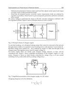
As it may be seen also in Fig. 1 the antenna receives radiated disturbance from EUT directly
but also by reflected wave from the reference ground plane, which ensures equivalent
conditions for all test sites.

EUT
height
1 - 4 m
rotating
0-360°
height

0,8m
measuring
receiver
antenna
mast
turntable
measuring distance D
reference
ground floor

Fig. 1. Scheme of radiated EMI measurement

Measured electromagnetic wave from the EUT is in the point of receiving antenna given by
vector sum of direct and reflected wave. Resulting phase of the sum is changing with the
varying height over the reference ground plane. Since the maximal radiated disturbance
must be found receiving antenna must change its height in the range of 1 m to 4 m and also
EUT must rotate to record all directions of possible radiations.
The measurement must be executed for both polarizations of receiving antenna – horizontal
and vertical. The radiated disturbance must be recorded in frequency range of 30 MHz to
1000 MHz and a quasi-peak value of this disturbance must be measured by a quasi-peak
detector. Such a value does not depend only on amplitude of the measured voltage but also
on its repetition frequency, so the resulting value is relative to voltage-time area of
disturbing signal.
So, concerning the radiated EMI measurement, it shall be found by the maximal radiated
disturbance is given:
 certain arrangement of EUT;
 certain turn of EUT;
 certain height of receiving antenna;
 certain polarization of receiving antenna;
 certain frequency of radiated disturbance.

If such a maximal value does not exceed the given disturbance limit value for the given
electric device, the EUT can be stated as electromagnetic compatible in terms of radiated
disturbance.

2.2 Uncertainty of measurement
In general, uncertainty of the measurement is as important as the result of measurement
itself. The term uncertainty represents a region about an observed value of a measured
quantity, which is likely to contain the true value of that quantity. The uncertainty describes
deficiencies of quantity knowledge. There are many potential uncertainty contributions,
which influence the uncertainty of measurement and which cannot be independent.
The standard CISPR 16-4-2 (CISPR 16-4-2) knows and quantifies following 17 uncertainty
contributions that influence the radiated EMI measurement:
 receiver reading;
 attenuation between antenna and receiver;
 antenna factor;
 receiver corrections for sine-wave voltage;
 receiver corrections for pulse amplitude corrections;
 receiver corrections for pulse repetition rate response;
 receiver corrections for noise floor proximity;
 mismatch between antenna and receiver;
 antenna factor frequency interpolation;
 antenna factor height deviations;
 directivity difference of antenna ;
 phase centre location of antenna;
 cross-polarisation of antenna;
 balance of antenna;
 test site imperfections;
 measuring distance between EUT and antenna;
 table or EUT height.
It is important to note, that despite the fact that most of these contributions do not influence

the result of measurement, they affect its uncertainty. The combined standard uncertainty
may be computed using Gauss’s law on the distribution of uncertainty:


 


i
iic
xucu
22
(1)

where c
i
is the sensitivity coefficient and u(x
i
) the standard uncertainty in decibel of i-th
contribution x
i
. The expanded measurement uncertainty may be calculated as:


c
uU 2

(2)
Theinterferencebetweengroundplaneandreceiving
antennaanditseffectontheradiatedEMImeasurementuncertainty 217
2. Radiated EMI measurement

2.1 Principle of measurement
A principle of the radiated EMI measurement given by (CISPR 16-2-3) is shown in Fig. 1.
The intensity of electric field, generated by EUT, is scanned by the receiving antenna and
measured by a rf measuring receiver. The measurement is executed in an open area test site,
but it may be performed also in shielded chambers to suppress ambient disturbing signals.
As it may be seen also in Fig. 1 the antenna receives radiated disturbance from EUT directly
but also by reflected wave from the reference ground plane, which ensures equivalent
conditions for all test sites.

EUT
height
1 - 4 m
rotating
0-360°
height
0,8m
measuring
receiver
antenna
mast
turntable
measuring distance D
reference
ground floor

Fig. 1. Scheme of radiated EMI measurement

Measured electromagnetic wave from the EUT is in the point of receiving antenna given by
vector sum of direct and reflected wave. Resulting phase of the sum is changing with the

varying height over the reference ground plane. Since the maximal radiated disturbance
must be found receiving antenna must change its height in the range of 1 m to 4 m and also
EUT must rotate to record all directions of possible radiations.
The measurement must be executed for both polarizations of receiving antenna – horizontal
and vertical. The radiated disturbance must be recorded in frequency range of 30 MHz to
1000 MHz and a quasi-peak value of this disturbance must be measured by a quasi-peak
detector. Such a value does not depend only on amplitude of the measured voltage but also
on its repetition frequency, so the resulting value is relative to voltage-time area of
disturbing signal.
So, concerning the radiated EMI measurement, it shall be found by the maximal radiated
disturbance is given:
 certain arrangement of EUT;
 certain turn of EUT;
 certain height of receiving antenna;
 certain polarization of receiving antenna;
 certain frequency of radiated disturbance.
If such a maximal value does not exceed the given disturbance limit value for the given
electric device, the EUT can be stated as electromagnetic compatible in terms of radiated
disturbance.

2.2 Uncertainty of measurement
In general, uncertainty of the measurement is as important as the result of measurement
itself. The term uncertainty represents a region about an observed value of a measured
quantity, which is likely to contain the true value of that quantity. The uncertainty describes
deficiencies of quantity knowledge. There are many potential uncertainty contributions,
which influence the uncertainty of measurement and which cannot be independent.
The standard CISPR 16-4-2 (CISPR 16-4-2) knows and quantifies following 17 uncertainty
contributions that influence the radiated EMI measurement:
 receiver reading;
 attenuation between antenna and receiver;

 antenna factor;
 receiver corrections for sine-wave voltage;
 receiver corrections for pulse amplitude corrections;
 receiver corrections for pulse repetition rate response;
 receiver corrections for noise floor proximity;
 mismatch between antenna and receiver;
 antenna factor frequency interpolation;
 antenna factor height deviations;
 directivity difference of antenna ;
 phase centre location of antenna;
 cross-polarisation of antenna;
 balance of antenna;
 test site imperfections;
 measuring distance between EUT and antenna;
 table or EUT height.
It is important to note, that despite the fact that most of these contributions do not influence
the result of measurement, they affect its uncertainty. The combined standard uncertainty
may be computed using Gauss’s law on the distribution of uncertainty:


 


i
iic
xucu
22
(1)

where c

i
is the sensitivity coefficient and u(x
i
) the standard uncertainty in decibel of i-th
contribution x
i
. The expanded measurement uncertainty may be calculated as:


c
uU 2 (2)
MicrowaveandMillimeterWaveTechnologies:ModernUWBantennasandequipment218
and it should be less than U
CISPR
, which is given by standard CISPR 16-4-2 and which is
5.2dB. If the uncertainty U is greater than U
CISPR
all the measurement results have to be
increased by the difference (U-U
CISPR
).

3. Receiving antennas

In order to obtain the radiated EMI measurement we should use antennas of various types.
An antenna transforms intensity of electromagnetic field to voltage, which is measurable by
the measuring receiver. To get the exact value of field intensity, tuned half-wave dipoles
shall be used. The dipoles represent basic type of line antennas, more details can be found in
(Balanis, 1997).
But nowadays, it is customary to use broadband antennas (biconical, log-periodic, Bilog or

horn antenna) to save measurement time. These antennas shall satisfy the standard
requirements (CISPR 16-1-4):
 the antennas shall be plane polarized;
 the main lobe of their radiation pattern shall be such that the response in the direction
of the direct wave and that in the direction of the wave reflected from the ground do
not differ by more than 1 dB;
 the voltage standing-wave ratio of the antenna with the antenna feeder connected and
measured from the receiver and shall not exceed 2.0 to 1;
Despite the fact that antennas satisfy the mentioned requirements they bring into
measurement additional errors, which increase the whole uncertainty of such a
measurement.
Broadband Bilog antennas are widely used in radiated emission measurements. They
represent combinations of biconical antenna and log-periodic dipole array, so they are able
to cover the frequency range from 30 MHz to 3 GHz (Van Dijk, 2005). By using the proper
geometry it is possible to achieve small dimensions of the antenna also at lower frequencies,
which is given by the bow-tie part of antenna. On the other hand the log-periodic part
determines the antenna properties at higher frequencies (usually over 200 MHz).
In presence of E field, voltage V is induced across a 50  load at the feed point of the
antenna. Then antenna factor AF represents the ratio between the field strength of an
incident plane wave E
in
and induced voltage V:


V
E
AF
in

(3)

or expressed in dB terms:


     
dBVdBE
V
E
dBAF
in
in

10
log20
(4)

Generally antenna factor AF may be expressed also by its parameter:


GZ
AF
2
480


 (5)
where Z is load impedance of antenna, l is a wavelength and G is a gain. Such an AF is free
space antenna factor determined on basis of the assumption that the antenna is located in
free space. In practice, radiated EMI measurements are always performed in presence of a
perfectly conducting ground plane. Since antenna like Bilog has large dimensions, there is a

not negligible effect of ground plane on antenna properties and also on antenna factor. In
this case antenna factor is known as a standard site method antenna factor. This parameter
may be obtained theoretically from the standard site attenuation A(dB) using the following
expression (Kodali, 1996):







dBAVmdBEfdBAF
DSSM

1
max
5.046.24log10)(

(5)

where f is frequency in MHz, E
D
max
is the maximum E field at the receiving antenna position
during scanning (from 1 m to 4 m height) for a half-wave dipole with 1 pW of radiated
power.
Other important parameter is the radiation pattern. It refers to the directional (angular)
dependence of radiation from the antenna. It is generally known that radiation pattern of
half-wave dipole is constant in H plane, but in E plane it is a figure-of-eight pattern. So the
directivity F given by sphere angles (


,

) can be expressed as:


 






sin
cos
2
cos
sin
2
coscos
2
cos
,






















klkl
F
(6)

where k is wave number (k=2/) and l the length of the dipole (in case of half-wave dipole
l=/2). Unfortunately, the radiation patterns of other (broadband) antennas are not known.
In addition they vary with changing frequency.

4. Modelling

The whole antenna analysis was executed by means of numerical methods – analytical
methods are suitable just for simple problems, while measurement is always affected by
auxiliary equipment. Numerical methods can be divided into three categories: frequency
domain, time domain and eigenmode or modal solvers. For antenna analysis the most
suitable method are solvers in frequency domain. The method of moments (Harrington,
1993) was chosen to analyse the problems.

The numerical model must be created at first to implement analysis by means of numerical
simulations. Interaction between dipole antenna and ground plane is known generally, so
we focused on popular broadband Bilog antenna. The Bilog antenna analysed in this
contribution is 785 mm long and 1660 mm wide, with 15 pairs of dipole elements and a
bow-tie part. The scale factor

and the spacing factor

of log-periodic dipole array
elements are 0.855 and 0.13 (the longest dipole element is 640 mm long). The bow-tie
element has the flare angle 37°, the height of triangle is 775 mm and height of feed point is
55 mm. The numerical model of such an antenna is shown in Fig. 2. The presented model is
a wire model – wire replacement of antenna – so the model consists just of wire segments.
Theinterferencebetweengroundplaneandreceiving
antennaanditseffectontheradiatedEMImeasurementuncertainty 219
and it should be less than U
CISPR
, which is given by standard CISPR 16-4-2 and which is
5.2dB. If the uncertainty U is greater than U
CISPR
all the measurement results have to be
increased by the difference (U-U
CISPR
).

3. Receiving antennas

In order to obtain the radiated EMI measurement we should use antennas of various types.
An antenna transforms intensity of electromagnetic field to voltage, which is measurable by
the measuring receiver. To get the exact value of field intensity, tuned half-wave dipoles

shall be used. The dipoles represent basic type of line antennas, more details can be found in
(Balanis, 1997).
But nowadays, it is customary to use broadband antennas (biconical, log-periodic, Bilog or
horn antenna) to save measurement time. These antennas shall satisfy the standard
requirements (CISPR 16-1-4):
 the antennas shall be plane polarized;
 the main lobe of their radiation pattern shall be such that the response in the direction
of the direct wave and that in the direction of the wave reflected from the ground do
not differ by more than 1 dB;
 the voltage standing-wave ratio of the antenna with the antenna feeder connected and
measured from the receiver and shall not exceed 2.0 to 1;
Despite the fact that antennas satisfy the mentioned requirements they bring into
measurement additional errors, which increase the whole uncertainty of such a
measurement.
Broadband Bilog antennas are widely used in radiated emission measurements. They
represent combinations of biconical antenna and log-periodic dipole array, so they are able
to cover the frequency range from 30 MHz to 3 GHz (Van Dijk, 2005). By using the proper
geometry it is possible to achieve small dimensions of the antenna also at lower frequencies,
which is given by the bow-tie part of antenna. On the other hand the log-periodic part
determines the antenna properties at higher frequencies (usually over 200 MHz).
In presence of E field, voltage V is induced across a 50  load at the feed point of the
antenna. Then antenna factor AF represents the ratio between the field strength of an
incident plane wave E
in
and induced voltage V:


V
E
AF

in

(3)

or expressed in dB terms:


     
dBVdBE
V
E
dBAF
in
in

10
log20
(4)

Generally antenna factor AF may be expressed also by its parameter:


GZ
AF
2
480


 (5)
where Z is load impedance of antenna, l is a wavelength and G is a gain. Such an AF is free

space antenna factor determined on basis of the assumption that the antenna is located in
free space. In practice, radiated EMI measurements are always performed in presence of a
perfectly conducting ground plane. Since antenna like Bilog has large dimensions, there is a
not negligible effect of ground plane on antenna properties and also on antenna factor. In
this case antenna factor is known as a standard site method antenna factor. This parameter
may be obtained theoretically from the standard site attenuation A(dB) using the following
expression (Kodali, 1996):







dBAVmdBEfdBAF
DSSM

1
max
5.046.24log10)(

(5)

where f is frequency in MHz, E
D
max
is the maximum E field at the receiving antenna position
during scanning (from 1 m to 4 m height) for a half-wave dipole with 1 pW of radiated
power.
Other important parameter is the radiation pattern. It refers to the directional (angular)

dependence of radiation from the antenna. It is generally known that radiation pattern of
half-wave dipole is constant in H plane, but in E plane it is a figure-of-eight pattern. So the
directivity F given by sphere angles (

,

) can be expressed as:


 






sin
cos
2
cos
sin
2
coscos
2
cos
,






















klkl
F
(6)

where k is wave number (k=2/) and l the length of the dipole (in case of half-wave dipole
l=/2). Unfortunately, the radiation patterns of other (broadband) antennas are not known.
In addition they vary with changing frequency.

4. Modelling

The whole antenna analysis was executed by means of numerical methods – analytical
methods are suitable just for simple problems, while measurement is always affected by
auxiliary equipment. Numerical methods can be divided into three categories: frequency

domain, time domain and eigenmode or modal solvers. For antenna analysis the most
suitable method are solvers in frequency domain. The method of moments (Harrington,
1993) was chosen to analyse the problems.
The numerical model must be created at first to implement analysis by means of numerical
simulations. Interaction between dipole antenna and ground plane is known generally, so
we focused on popular broadband Bilog antenna. The Bilog antenna analysed in this
contribution is 785 mm long and 1660 mm wide, with 15 pairs of dipole elements and a
bow-tie part. The scale factor

and the spacing factor

of log-periodic dipole array
elements are 0.855 and 0.13 (the longest dipole element is 640 mm long). The bow-tie
element has the flare angle 37°, the height of triangle is 775 mm and height of feed point is
55 mm. The numerical model of such an antenna is shown in Fig. 2. The presented model is
a wire model – wire replacement of antenna – so the model consists just of wire segments.
MicrowaveandMillimeterWaveTechnologies:ModernUWBantennasandequipment220
This model is composed of 191 segments, and elements of antenna are connected to each
other by non-radiating transmission lines.

Fig. 2. The numerical model of analysed Bilog antenna.

To use these models, at first we have to validate the numerical model of the Bilog antenna.
That means to verify that the obtained results copy sufficiently the properties of real
antenna. The antenna factor values are obtained by simulation by placing a source of
electromagnetic field e.g. short dipole antenna at adequate distance (ca. 100 m) away from
the receiving Bilog antenna. Then antenna factor is given as ratio between known E field
values E
in
and computed induced voltage at antenna output V (Chen & Lin, 2003). The

comparison of obtained simulated values of free space antenna factor with the measured
values provided by manufacturer is shown in Fig. 3. There is a good correlation between
measured and simulated antenna factor values, the small differences below 200 MHz can be
caused by omission of balun (balanced-unbalanced network) in case of simulations. At
higher frequencies, the effect of sequential activation of log-periodic dipole elements may be
seen.


















Fig. 3. Comparison of measured and simulated values of antenna factor of Bilog antenna.
100 1000
6
8
10
12

14
16
18
20
22
24
26
AF (dB/m)
f (MHz)
measured in free space by producer
measured by standard site method
- horizontal polarisation
measured by standard site method
- vertical polarisation
simulation of free space antenna factor
Also the simulated radiation patterns of Bilog antenna were compared with measured ones
at discrete frequencies. The differences are mainly in back lobe (see Fig. 4), which may be
caused by antenna feeder presence during the measurement, or by small errors in numerical
computation.

(a) (b)
Fig. 4. Comparison of measured and simulated radiation patterns of Bilog antenna at
200 MHz (a) in E plane, (b) in H plane.

5. Methods

From all mentioned uncertainty contributions two of them affected by ground plane
presence were chosen for further analysis:
 antenna factor height deviations;
 directivity difference of antenna.
It is known that the presence of ground plane affects the input impedance Z of every
antenna. The change of impedance cause change of induced voltage V on antenna, and
consequently according to (3) also change of antenna factor AF. This variation may be
expressed as error of antenna factor

AF:


FSh
AFAFAF 
(7)

where AF
FS
is antenna factor of antenna in free space and AF
h
antenna factor of the same
antenna, calculated by the same conditions, in the height h over the reference ground plane.

It is necessary to ensure the identical height of both antennas (transmitting short dipole and
receiving analysed antenna) during the antenna factor calculation. Unfortunately, the error

AF is not constant. It changes with varying height of antenna and also with frequency.
Therefore it is necessary to consider with range of errors, obtained as intersection of all the
errors for height interval from 1 m to 4 m.
Note that the change of antenna impedance due to height variation may cause also
additional error in mismatch between antenna and receiver.
Broadband antennas have radiation patterns different from the half-wave dipole and they
are additionally frequency dependent. At lower frequencies, the radiation pattern of Bilog
antenna is similar to the pattern of half-wave dipole. But with increasing frequency of
0
30
60
90
120
150
180
210
240
270
300
330
0.0
0.2
0.4
0.6
0.8
1.0
0.0

0.2
0.4
0.6
0.8
1.0
BiLog - measured
BiLog - simulated
Halfwave dipole
0
30
60
90
120
150
180
210
240
270
300
330
0.0
0.2
0.4
0.6
0.8
1.0
0.0
0.2
0.4
0.6

0.8
1.0
Theinterferencebetweengroundplaneandreceiving
antennaanditseffectontheradiatedEMImeasurementuncertainty 221
This model is composed of 191 segments, and elements of antenna are connected to each
other by non-radiating transmission lines.

Fig. 2. The numerical model of analysed Bilog antenna.

To use these models, at first we have to validate the numerical model of the Bilog antenna.
That means to verify that the obtained results copy sufficiently the properties of real
antenna. The antenna factor values are obtained by simulation by placing a source of
electromagnetic field e.g. short dipole antenna at adequate distance (ca. 100 m) away from
the receiving Bilog antenna. Then antenna factor is given as ratio between known E field
values E
in
and computed induced voltage at antenna output V (Chen & Lin, 2003). The
comparison of obtained simulated values of free space antenna factor with the measured
values provided by manufacturer is shown in Fig. 3. There is a good correlation between
measured and simulated antenna factor values, the small differences below 200 MHz can be
caused by omission of balun (balanced-unbalanced network) in case of simulations. At
higher frequencies, the effect of sequential activation of log-periodic dipole elements may be
seen.

Fig. 3. Comparison of measured and simulated values of antenna factor of Bilog antenna.
100 1000
6
8
10
12
14
16
18
20
22
24
26
AF (dB/m)
f (MHz)
measured in free space by producer
measured by standard site method
- horizontal polarisation
measured by standard site method

- vertical polarisation
simulation of free space antenna factor
Also the simulated radiation patterns of Bilog antenna were compared with measured ones
at discrete frequencies. The differences are mainly in back lobe (see Fig. 4), which may be
caused by antenna feeder presence during the measurement, or by small errors in numerical
computation.













(a) (b)
Fig. 4. Comparison of measured and simulated radiation patterns of Bilog antenna at
200 MHz (a) in E plane, (b) in H plane.

5. Methods

From all mentioned uncertainty contributions two of them affected by ground plane
presence were chosen for further analysis:
 antenna factor height deviations;
 directivity difference of antenna.
It is known that the presence of ground plane affects the input impedance Z of every

antenna. The change of impedance cause change of induced voltage V on antenna, and
consequently according to (3) also change of antenna factor AF. This variation may be
expressed as error of antenna factor

AF:


FSh
AFAFAF 
(7)

where AF
FS
is antenna factor of antenna in free space and AF
h
antenna factor of the same
antenna, calculated by the same conditions, in the height h over the reference ground plane.
It is necessary to ensure the identical height of both antennas (transmitting short dipole and
receiving analysed antenna) during the antenna factor calculation. Unfortunately, the error

AF is not constant. It changes with varying height of antenna and also with frequency.
Therefore it is necessary to consider with range of errors, obtained as intersection of all the
errors for height interval from 1 m to 4 m.
Note that the change of antenna impedance due to height variation may cause also
additional error in mismatch between antenna and receiver.
Broadband antennas have radiation patterns different from the half-wave dipole and they
are additionally frequency dependent. At lower frequencies, the radiation pattern of Bilog
antenna is similar to the pattern of half-wave dipole. But with increasing frequency of
0
30

60
90
120
150
180
210
240
270
300
330
0.0
0.2
0.4
0.6
0.8
1.0
0.0
0.2
0.4
0.6
0.8
1.0
BiLog - measured
BiLog - simulated
Halfwave dipole
0
30
60
90
120

150
180
210
240
270
300
330
0.0
0.2
0.4
0.6
0.8
1.0
0.0
0.2
0.4
0.6
0.8
1.0
MicrowaveandMillimeterWaveTechnologies:ModernUWBantennasandequipment222
radiation the main lobe of radiation pattern becomes more dominant, so there is less
similarity between two radiation patterns (see Fig. 5). Hence, there is higher probability that
error caused by the real radiation pattern of Bilog antenna is higher than at lower
frequencies and the using of such antennas introduces additional error into the
measurement.


Fig. 5. Radiation pattern of Bilog antenna at frequencies 30 MHz, 300 MHz and 1000 MHz.

In addition, the ground plane also affects the directivity of the antenna. The variation of

radiation pattern may be expressed as well simply as the error of antenna factor. If the
source of radiation is not situated in front of analysed antenna in direction of maximal
radiation (zero angle-wise), but it is moved so that radiation from itself affects the analysed
antenna with angles (

,

), we obtain the real antenna factor of antenna AF:












,, FdBAFAF  (8)

where AF(dB) is known antenna factor and F is directivity of analysed antenna. Then the
error, obtained by replacing the half-wave dipole antenna by broadband antenna, may be
expressed as error of antenna factor

AF defined as:







KAFAFdBAF
D


,,)( (9)

where AF and AF
D
are antenna factors at the same angles of incidence given by angles (

,

).
The dependence of antenna factor of half-wave dipole antenna may be obtained by
substituting (6) into (8). The parameter K is a correction for neglecting the difference
between the values of antenna factors of these antennas.
Since receiving antenna varies its height with respect to height of tested equipment during
the measurement from 1 to 4 m, angles of incidence of disturbing electromagnetic waves on
measuring antenna vary their values as well. If tested object is assumed to be in 1 m height
and the measuring distance is standard (CISPR 16-1-4) recommended 10 m the angle of
incidence of direct wave varies from 0° to 17°. In case of shorter distances e.g. 3 m these
angles may increase up to 45°. If we consider not only the direct wave incident on the
antenna, but also the wave reflected from the reference ground plane, angles of incidence
are from 0° up to 27°. Similarly for 3 m measuring distance we have to consider a range of
possible angles of incidence up to 60° or for 30 m just up to 9.5°. The possible errors of
antenna factor, which may be included into the entire uncertainty, are shown in Fig. 6 and 7.
It is necessary to consider the range of errors, because the real error may vary in value

according to angle of incidence, which is unknown.


















Fig. 6. Possible errors of antenna factor caused by directivity for horizontally polarised Bilog
and for different measuring distances

Fig. 7. Possible errors of antenna factor caused by directivity for vertically polarised Bilog
and for different measuring distances

100 200 300 400 500 600 700 800 900 1000
-5
-4
-3
-2
-1
0
1
2
3
AF (dB)
f (MHz)
3m 10m 30m
100 200 300 400 500 600 700 800 900 1000
-7
-6
-5
-4

-3
-2
-1
0
1
2
3
AF (dB)
f (MHz)
3m 10m 30m
Theinterferencebetweengroundplaneandreceiving
antennaanditseffectontheradiatedEMImeasurementuncertainty 223
radiation the main lobe of radiation pattern becomes more dominant, so there is less
similarity between two radiation patterns (see Fig. 5). Hence, there is higher probability that
error caused by the real radiation pattern of Bilog antenna is higher than at lower
frequencies and the using of such antennas introduces additional error into the
measurement.


Fig. 5. Radiation pattern of Bilog antenna at frequencies 30 MHz, 300 MHz and 1000 MHz.

In addition, the ground plane also affects the directivity of the antenna. The variation of
radiation pattern may be expressed as well simply as the error of antenna factor. If the
source of radiation is not situated in front of analysed antenna in direction of maximal
radiation (zero angle-wise), but it is moved so that radiation from itself affects the analysed
antenna with angles (

,

), we obtain the real antenna factor of antenna AF:











,, FdBAFAF


(8)

where AF(dB) is known antenna factor and F is directivity of analysed antenna. Then the
error, obtained by replacing the half-wave dipole antenna by broadband antenna, may be
expressed as error of antenna factor

AF defined as:






KAFAFdBAF
D



,,)( (9)

where AF and AF
D
are antenna factors at the same angles of incidence given by angles (

,

).
The dependence of antenna factor of half-wave dipole antenna may be obtained by
substituting (6) into (8). The parameter K is a correction for neglecting the difference
between the values of antenna factors of these antennas.
Since receiving antenna varies its height with respect to height of tested equipment during
the measurement from 1 to 4 m, angles of incidence of disturbing electromagnetic waves on
measuring antenna vary their values as well. If tested object is assumed to be in 1 m height
and the measuring distance is standard (CISPR 16-1-4) recommended 10 m the angle of
incidence of direct wave varies from 0° to 17°. In case of shorter distances e.g. 3 m these
angles may increase up to 45°. If we consider not only the direct wave incident on the
antenna, but also the wave reflected from the reference ground plane, angles of incidence
are from 0° up to 27°. Similarly for 3 m measuring distance we have to consider a range of
possible angles of incidence up to 60° or for 30 m just up to 9.5°. The possible errors of
antenna factor, which may be included into the entire uncertainty, are shown in Fig. 6 and 7.
It is necessary to consider the range of errors, because the real error may vary in value
according to angle of incidence, which is unknown.

Fig. 6. Possible errors of antenna factor caused by directivity for horizontally polarised Bilog
and for different measuring distances

Fig. 7. Possible errors of antenna factor caused by directivity for vertically polarised Bilog
and for different measuring distances

100 200 300 400 500 600 700 800 900 1000
-5
-4
-3
-2
-1
0
1
2
3
AF (dB)
f (MHz)
3m 10m 30m
100 200 300 400 500 600 700 800 900 1000
-7
-6
-5
-4
-3
-2
-1
0
1

2
3
AF (dB)
f (MHz)
3m 10m 30m
MicrowaveandMillimeterWaveTechnologies:ModernUWBantennasandequipment224
Since the radiation pattern of tested equipment and then also the angle of incidence are
mostly unknown, we take into account that disturbing electromagnetic field may be
received by measuring antenna with the same probability with any angle from given range.
Hence, it is necessary to rotate the source of radiation around the analysed measuring
antenna with these angles and record the maximal variations (positive and negative) in
comparison with zero angle of incidence. This process was performed at multiple discrete
points of frequency range of our interest from 30 to 1000 MHz and for both polarizations of
antenna. The result is the error of antenna factor

AF, respectively its frequency
dependence, which represents one of contributions to entire uncertainty of the radiated EMI
measurement. The error

AF is not single-valued, it may be arbitrary between maximal and
minimal range, but we have to consider the maximal error in order to calculate the
measurement uncertainty.

6. Results

The perfect ground plane presence near the Bilog antenna affects its input impedance as
well as its antenna factor. But it also affects its radiation pattern of Bilog antenna. To obtain
the error

AF of Bilog antenna, which is influenced by ground plane presence, we have to

modify the numerical model of the antenna. Instead of inserting the ground plane into the
model, we make use of the mirror principle and below the Bilog we locate its mirror image
in distance of double height over the ground plane. In such cases it is necessary to get the
maximal and minimal values of error

AF at different angles of incidence, which are
dependent on the antenna height over the ground plane.




















Fig. 8. Possible errors of antenna factor for a horizontally polarized Bilog placed in height h
over the ground plane

200 400 600 800 1000
-1.0
-0.8
-0.6
-0.4
-0.2
0.0
0.2
0.4
0.6
0.8
1.0
 AF (dB)
f (MHz)
h = 1m
h = 2m
h = 3m
h = 4m
h = 1÷4m scan

Fig. 9. Possible errors of antenna factor for a horizontally polarized Bilog placed in height h
over the ground plane

As the antenna varies its height above the reference ground plane, its antenna factor varies
as well. This variation

AF is shown in Fig. 8 and 9 according to (7). The error is strongly
frequency dependant and it is maximal ±0.8 dB in case of the lowest height of antenna
h = 1 m. This is when the mutual coupling between the antenna and the ground plane is
maximal. The error is large in the frequency range below 200 MHz, which is the active range
of bow-tie part of antenna. The log-periodical part causes a smaller error when mainly
vertically polarised. It is consistent with the previous analysis of biconical or log-periodical
antennas (Chen & Foegelle 1998), (Chen et al. 1999).
The error

AF is dependent also on the angle of incidence. While at zero angle of incidence
the error is zero due to correction K, with increasing angles of incidence the error

AF also
generally increases in value. As we can see in Fig. 6 and 7 the worst situation occurs at short
measuring distances of 3 m. A better situation occurs in case of horizontally polarized
antenna, the possible error is up to ±1.4 dB. In case of vertical polarized antenna the error is
up to ±2 dB. With increasing measuring distance the values of error


AF descends, at 10 m
the maximal error is ±4.1 dB or ±6 dB and at 30 m distance ±0.2 dB or ±0.8 dB for both
polarizations. Such errors are visibly frequency dependent and mostly negative, which
means that received signal is smaller than expected
The effect of ground plane presence on directional patterns of Bilog antenna we may be seen
in Fig. 10. With increasing height over the ground plane the directional pattern of Bilog
antenna becomes smoother – it resembles the directional pattern in free space. On the other
hand at low heights also the main lobe of the pattern is crinkled. Even though the ground
plane influence on radiation pattern of Bilog cannot be overlooked, this effect is not so
evident on frequency characteristics of error

AF as a whole, as it is seen in Fig. 11 and 12.
More significant is the interference of bow-tie part of Bilog with ground plane in the
frequency range from 100 to 200 MHz that causes higher error of antenna factor. The effect
200 400 600 800 1000
-1.0
-0.8
-0.6
-0.4
-0.2
0.0
0.2
0.4
0.6
0.8
1.0
h = 1m
h = 2m
h = 3m

h = 4m
h = 1÷4m scan
 AF (dB)
f (MHz)
Theinterferencebetweengroundplaneandreceiving
antennaanditseffectontheradiatedEMImeasurementuncertainty 225
Since the radiation pattern of tested equipment and then also the angle of incidence are
mostly unknown, we take into account that disturbing electromagnetic field may be
received by measuring antenna with the same probability with any angle from given range.
Hence, it is necessary to rotate the source of radiation around the analysed measuring
antenna with these angles and record the maximal variations (positive and negative) in
comparison with zero angle of incidence. This process was performed at multiple discrete
points of frequency range of our interest from 30 to 1000 MHz and for both polarizations of
antenna. The result is the error of antenna factor

AF, respectively its frequency
dependence, which represents one of contributions to entire uncertainty of the radiated EMI
measurement. The error

AF is not single-valued, it may be arbitrary between maximal and
minimal range, but we have to consider the maximal error in order to calculate the
measurement uncertainty.

6. Results

The perfect ground plane presence near the Bilog antenna affects its input impedance as
well as its antenna factor. But it also affects its radiation pattern of Bilog antenna. To obtain
the error

AF of Bilog antenna, which is influenced by ground plane presence, we have to

modify the numerical model of the antenna. Instead of inserting the ground plane into the
model, we make use of the mirror principle and below the Bilog we locate its mirror image
in distance of double height over the ground plane. In such cases it is necessary to get the
maximal and minimal values of error

AF at different angles of incidence, which are
dependent on the antenna height over the ground plane.




















Fig. 8. Possible errors of antenna factor for a horizontally polarized Bilog placed in height h
over the ground plane

200 400 600 800 1000
-1.0
-0.8
-0.6
-0.4
-0.2
0.0
0.2
0.4
0.6
0.8
1.0
 AF (dB)
f (MHz)
h = 1m
h = 2m
h = 3m
h = 4m
h = 1÷4m scan

Fig. 9. Possible errors of antenna factor for a horizontally polarized Bilog placed in height h
over the ground plane

As the antenna varies its height above the reference ground plane, its antenna factor varies
as well. This variation

AF is shown in Fig. 8 and 9 according to (7). The error is strongly
frequency dependant and it is maximal ±0.8 dB in case of the lowest height of antenna
h = 1 m. This is when the mutual coupling between the antenna and the ground plane is
maximal. The error is large in the frequency range below 200 MHz, which is the active range
of bow-tie part of antenna. The log-periodical part causes a smaller error when mainly
vertically polarised. It is consistent with the previous analysis of biconical or log-periodical
antennas (Chen & Foegelle 1998), (Chen et al. 1999).
The error

AF is dependent also on the angle of incidence. While at zero angle of incidence
the error is zero due to correction K, with increasing angles of incidence the error

AF also
generally increases in value. As we can see in Fig. 6 and 7 the worst situation occurs at short
measuring distances of 3 m. A better situation occurs in case of horizontally polarized
antenna, the possible error is up to ±1.4 dB. In case of vertical polarized antenna the error is
up to ±2 dB. With increasing measuring distance the values of error


AF descends, at 10 m
the maximal error is ±4.1 dB or ±6 dB and at 30 m distance ±0.2 dB or ±0.8 dB for both
polarizations. Such errors are visibly frequency dependent and mostly negative, which
means that received signal is smaller than expected
The effect of ground plane presence on directional patterns of Bilog antenna we may be seen
in Fig. 10. With increasing height over the ground plane the directional pattern of Bilog
antenna becomes smoother – it resembles the directional pattern in free space. On the other
hand at low heights also the main lobe of the pattern is crinkled. Even though the ground
plane influence on radiation pattern of Bilog cannot be overlooked, this effect is not so
evident on frequency characteristics of error

AF as a whole, as it is seen in Fig. 11 and 12.
More significant is the interference of bow-tie part of Bilog with ground plane in the
frequency range from 100 to 200 MHz that causes higher error of antenna factor. The effect
200 400 600 800 1000
-1.0
-0.8
-0.6
-0.4
-0.2
0.0
0.2
0.4
0.6
0.8
1.0
h = 1m
h = 2m
h = 3m

h = 4m
h = 1÷4m scan
 AF (dB)
f (MHz)