Quantitative Techniques for Competition and Antitrust Analysis by Peter Davis and Eliana Garcés_13 pot

9.1. Demand System Estimation: Models of Continuous Choice 443
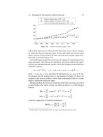
Table 9.2. IV estimation results based on forty-four observations.
Robust
Regressors Coefficient std. err. tP>jtj [95% Conf. interval]
ln.P
Sugar
/ 0.27 0.08 3.41 0.00 [0.43 0.11]
Quarter 1 0.10 0.01 9.23 0.00 [0.12 0.08]
Quarter 2 0.01 0.01 1.99 0.05 [0.02 0.00]
Quarter 3 0.01 0.00 3.71 0.00 [0.01 0.02]
Constant 8.69 0.25 34.71 0.00 [8.19 9.20]
R
2
D 0:80. The dependent variable in this regression is ln.Q
Sugar
/.
are a cost of producing sugar and will therefore ordinarily affect observed prices
according to economic theory (and also farmers!). On the other hand, given that
farmers are a small minority of the population and that the increase in their wages
is not likely to translate into material increases in sugar consumption, farm wages
are unlikely to materially affect the aggregate demand for sugar.
The 2SLS estimation proceeds in two stages:
1st-stage regression: ln P
t
D a b ln W
t
C 
1
q
1t
C 

2
q
2t
C 
3
q
3t
C "
t
;
2nd-stage regression: ln Q
t
D a b
b
ln P
t
C 
1
q
1t
C 
2
q
2t
C 
3
q
3t
C v
t

;
where W
t
is the farm wage at time t and
b
ln P
t
is the estimated log of price ob-
tained from the first-stage regression. Most statistical computer packages are able to
perform this procedure and in doing so provide the output from both regressions.
8
The quarterly dummies are also included in the first-stage regression since the
requirement for an instrument to be valid is that it is correlated with an endogenous
variable conditional on the included exogenous variables. Demand is itself seasonal,
so that the quarterly dummies are not correlated with prices conditional on the
included exogenous variables and hence are not valid instruments for prices, even
if they are valid instruments for themselves, i.e., can be treated as exogenous.
The results of the instrumental variable estimation are presented in table 9.2.
The resultsshowa lower coefficient for the price variable. The elasticity of demand
is now 0:27 and is below the previous OLS estimate. Because of data availability
on farm wages some observations had to be dropped so that the data for the two
regressions are not exactly the same. Nonetheless, formally a Durbin–Wu–Hausman
test could be used to test between the OLS and IV regression specifications (see
Greene 2000; Nakamura and Nakamura 1981). The central question is whether the
instruments are in fact successfully addressing the endogeneity bias problem that
motivated our use of them. Often inexperienced researchers use IV regression results
even if the resulting estimate moves the coefficient in the direction opposite to that
expected as a result of endogeneity bias.
8
STATA, for example, provides the “ivreg” command.

444 9. Demand System Estimation
Results in IV estimations should be carefully scrutinized because they will only be
reliable if the instrument chosen for the first-stage regression is a good instrument.
We know that for an instrument to be valid it must satisfy the two conditions:
(i) EŒ
t
j .X
t
;W
t
/ D 0 and (ii) EŒln.P
t
/ j .X
t
;W
t
/ ¤ 0;
where in our case X
t
D .1; q
1
;q
2
;q
3
/ are the exogenous regressors in the demand
equation and W
t
is the instrument, farm wages. As we described earlier, the first
of these conditions is difficult to test; however, one way to evaluate whether it

holds is to examine a picture of the estimated residuals against the regressors. We
should see no systematic patterns in the graphs—whatever the value of X
t
or W
t
the error term on average around those values should be mean zero. Such tests can
be formalized (see, for example, the specification tests due to Ramsey (1969)). But
there are limits to the extent to which this assumption can be tested since the model
will, to a considerable extent, actively impose this assumption on the data in order to
best derive the IV estimates obtained. A variety of potential IV results can certainly
be tested against each other and against specifications which use more instruments
than strictly necessary to achieve identification. But the reality is that the first of
these assumptions is ultimately quite difficult to test entirely convincingly and one
is likely to ultimately mainly rely on economic theory—at least to the extent that
the theory robustly tells us that, for example, a cost driver will generally not affect
consumer demand behavior and so will have no reason to be correlated with the
unobserved component of demand.
The second condition is easier to evaluate and the most popular method is to run a
regression of the potentially endogenous variable (here ln.P
t
/) on all the exogenous
explanatory variables in the demand equation and also the instruments, here ln.W
t
/.
To see whether the second condition holds, we examine the results of the following
“first-stage” regression:
P
t
D a b ln W
t

C q
1
C q
2
C q
3
C "
t
:
For the variable farm wage to be a good instrument, we want the coefficient b to
be robustly and significantly different from zero in this equation. If the instrument
does not have explanatory power in predicting the price, the predicted price used in
the second-stage regression will be poorly correlated with the actual price given the
other variables already included in the demand equation. In that case, the estimated
coefficient of the price variable in the second-stage regression will be imprecisely
estimated and indeed may not be distinguishable from zero. Even with “good instru-
ments” in the sense that they are conditionally correlated with the variable being
instrumented, we will expect the coefficient of an instrumented variable in an IV
regression to be lessprecisely estimated (have a higher standard error)than theanalo-
gous coefficient estimated using OLS (with the latter a meaningful comparison only
if in fact the OLS estimate is a valid one). IV estimation relaxes the assumptions
9.1. Demand System Estimation: Models of Continuous Choice 445
Table 9.3. First-stage regression results.
ln.Price/ Coefficient Std. err. tP>jtj [95% conf. interval]
Quarter 1 0.05 0.02 2.93 0.01 [0.01 0.08]
Quarter 2 0.00 0.01 0.53 0.60 [0.01 0.02]
Quarter 3 0.01 0.01 1.43 0.16 [0.02 0.00]
ln.Farm wage/ 1.13 0.12 9.71 0.00 [1.36 0.89]
Constant 4.94 0.18 27.47 0.00 [4.58 5.30]
required to get valid estimates but one must always remember it does so at a price:

lower precision. There will, as a result, be cases where the OLS estimates cannot be
rejected when compared with the IV estimates and may as a result be preferred.
Results for the first-stage regression for our example are shown in table 9.3.
First note that, as one would hope, the coefficient for the ln(Farm wage) variable
is significant and has a high t-statistic, indicating that it is precisely estimated.
However, note that the coefficient reported is rather surprising: its sign is negative!
The economic theory motivating our choice of instrument tells us that an increase in
costs should translate into higher prices as the supply curve shifts leftward. Indeed,
our aim in selecting an instrument is intuitively to use that instrument to allow us to
use only the variation in observed prices which we know is due to the variation in
the supply curve.
When conundrums such as this one arise, one should address them. While for
econometric theory purposes “conditional correlation” is all that is required to sup-
port the use of the instrument, one should not proceed further without understanding
why the data are behaving in an unexpected way. In this case, one may want to inves-
tigate, for example, whether farm wages have a trend that negatively correlates with
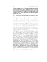
prices and for which we did not control. Figure 9.2 graphs farm wage data over
time. In particular, note that there is an upward trend in wages between 1995 and
2006 during the time that sugar prices fell. Clearly, while farm wages may still be
an important determinant of sugar prices, they are not likely to be a major factor
driving the price of sugar down. We must look elsewhere for an instrument that
helps explain the major source of variation in prices conditional on the exogenous
variables in the demand equation.
To search for a good instrument we must attempt to better understand the factors
that are driving sugar prices down over time. One possibility is that other costs
in the industry are falling dramatically. Alternatively, there may be an institutional
reason such as changes in the amount of subsidy offered to farmers or in the tariff or
quota system that governs the supply from imports. There may have been substantial
entry during the period. Another possibility is that the price change may be driven
by important demand factors that we have omitted thus far from our model. Perhaps

the taste for sugary products changed over time? Or perhaps substitutes (e.g., high-
fructose corn syrup) appeared and drove down prices?
446 9. Demand System Estimation
1992q1 1995q3 1999q1 2002q3 2006q1
Date
P
Farm wage
4.2
4.4
4.6
4.8
5.0
5.2
Figure 9.2. Farm wages plotted over time.
At this point we need to go back to our industry experts and descriptive analyses of
the industry to attempt to find possible explanations for the major variation in prices
and in particular the price decline. The data and regression results have provided
us with a puzzle which we need to solve by using industry expertise. Only once we
have thought hard about what in the industry is generating our data will we generally
be able to move forward to generating econometric results we can believe. It is for
this reason that we described in the introduction to this section that it is very rare for
an econometrician to be able to work in isolation late into the night with her existing
data set and generate sensible regression results without going back to think about
the nature and drivers of competition in an industry.
That said, we generally do not need to understand everything about the price-
setting process to obtain reliable demand estimates. In particular, in a demand esti-
mation exercise we are not trying to estimate the pricing equations that explain how
firms optimally choose their prices. Although the first-stage regression in a 2SLS
estimation may closely resemble the reduced form of the pricing equation in a struc-
tural model of prices and quantities (see chapter 6), it is not quite the same. We saw

in the previous chapters that factors affecting demand are included in the pricing
equation and so are cost data. However, the first-stage equation of the 2SLS regres-
sion is materially different from a reduced-form pricing equation in that we do not
need to have all the cost data: we really only need one good supply-side instrument
to identify the price coefficient in a homogeneous product demand equation.
9.1.2 Differentiated Products Demand Systems
Most markets do not consist of a single homogeneous product but are rather com-
posed of similar but differentiated goods that compete for customers. For instance,
in the market for shampoos there is not a single type of generic shampoo. Rather
there is a variety of brands and types of shampoo which consumers do not consider
9.1. Demand System Estimation: Models of Continuous Choice 447
absolutely equivalent. We must take such demand characteristics into account when
attempting to estimate demand in differentiated product markets. In particular, we
need to take account of the fact that consumers are choosing among different prod-
ucts for which they have different relative preferences and which will usually have
different prices. Differentiated product demand systems are therefore estimated as
a system of individual product demand equations, where the demand for a product
depends on its own price but also on the price of the other products in the market.
9.1.2.1 Log-Linear Demand Models
One popular differentiated product demand system is the log-linear demand system,
which is simply a set of log-linear demand functions, one for each product available
in the market. We label the products in the market j D 1;:::;J. In each case, the
quantity of the good purchased potentially depends on the prices of all the goods in
the market and also income y (Deaton and Muellbauer 1980b). Formally, we have
the following system of J equations:
ln Q
1t
D a
1
 b

11
ln P
1t
C b
12
ln P
2t
C :::: C b
1J
ln P
1J
C 
1
ln y
t
C 
1t
;
ln Q
2t
D a
2
 b
21
ln P
1t
C b
22
ln P
2t

CCb
2J
ln P
Jt
C 
2
ln y
t
C 
2t
;
:
:
:
ln Q
Jt
D a
2
 b
J1
ln P
1t
C b
J2
ln P
2t
CCb
JJ
ln P
Jt

C 
J
ln y
t
C 
Jt
:
Maximizing utility subject to a budget constraint will generically provide demand
equations which depend on the set of all prices and income (see, for example, Pollak
and Wales 1992). Clearly, with aggregate data we might use aggregate income as the
relevant variable for the demand equations (e.g., GDP). However, since many studies
focus on a particular sector of the economy, the consumer’s problem is often recast
and considered as a two-stage problem. At the first stage, we posit that consumers
decide how much money to spend on a category of goods—for example, beer—and
at the second stage we posit that the chosen level of expenditure is allocated across
the various products that the consumer must choose between, perhaps the different
brands of beer. Under particular assumptions on the shape of the utility function,
this two-stage process can be shown to be equivalent to solving a single one-stage
utility-maximization problem (see Deaton and Muellbauer 1980b; Gorman 1959;
Hausman et al. 1994). Using the two-stage interpretation, “expenditure” may be
used instead of income in the demand equations but the demand equations will then
be termed “conditional” demand equations as we are conditioning on a given level
of expenditure.
A well-known example of an such an exercise is Hausman et al. (1994). In fact,
those authors estimate a three-level choice model where consumers choose (1) the
level of expenditure on beer, (2) how to allocate that expenditure between three
broad categories of beer (respectively termed premium beer, popular beer, and light
448 9. Demand System Estimation
Table 9.4. Market segment conditional demand in the market for beer.
Premium Popular Light

Constant 0.501 4.021 1.183
(0.283) (0.560) (0.377)
log(Beer exp) 0.978 0.943 1.067
(0.011) (0.022) (0.015)
log(P
Premium
) 2.671 2.704 0.424
(0.123) (0.244) (0.166)
log(P
Popular
) 0.510 2.707 0.747
(0.097) (0.193) (0.127)
log(P
Light
) 0.701 0.518 2.424
(0.070) (0.140) (0.092)
Time 0.001 0.000 0.002
(0.000) (0.001) (0.000)
log(# of stores) 0.035 0.253 0.176
(0.016) (0.034) (0.023)
Number of observations = 101.
Source: Table 1, Hausman et al. (1994).
beer) which marketing studies had identified as market segments, and (3) how to
allocate expenditure between the various brands of beer within each of the segments.
At level (3), we could use the observed product level price and quantity data to
estimate our differentiated product demand system. However, in fact, since level (3)
is modeled as a choice of brands (e.g., Coors, Budweiser, Molsen, etc.), at levels
(1), (2), and (3) we would need to use price and quantity indices constructed from
underlying product-level data to give measures of price and quantity for each of the
brands or segments of the beer industry. For example, we might use a price index with

expenditure share weights forthe underlying prices within each segment s to produce
a segment-level price index, P
st
D
P
j
w
jt
p
jt
.
9
Similarly, we might choose to use
volumes of liquid to help aggregate over the brands to give segment-level quantity
indices.
10
Estimates of the second level of their demand system using price and quantity
indices are shown in table 9.4. At the second level of the choice tree, the demand
system is a conditional demand system because the amount of money to be spent
on beer has already been chosen at stage 1.
9
Expenditure shares can be defined as w
jt
D p
jt
q
jt
=
P
j

p
jt
q
jt
, where p represents prices and
q quantities.
10
Formally, Deaton and Muellbauer (1980b) show that there are “correct” price and quantity indices
which can be constructed for this process to preserve the multilevel models’ equivalence to a single
utility-maximization problem (under strong assumptions). In practice, the authors do not seem to have
settled on a universally best choice of price and quantity indices.
9.1. Demand System Estimation: Models of Continuous Choice 449
Since weare dealingwith alog-linear model,the b
jj
coefficientsprovide estimates
of the own-price elasticity of demand while the b
jk
(j ¤ k) parameters provide
estimates of the cross-price elasticities of demand. If we are using segment-level
data, we must be careful to place the correct interpretation on the elasticities. For
example, the results from table 9.4 suggest that the own-price elasticity of segment
demand is 2:6 for premium beer, 2:7 for popular beer, and 2:4 for light beer.
These price elasticities could be used as important evidence toward a formal test
of the hypothesis that each beer segment is a market in itself by performing a SSNIP
test. That said, generally, the price elasticity relevant for such a test would include
the indirect effect of prices through their effect on the total amount of expenditure
on beer. If the price of premium beer goes up, some consumption will be reallocated
to other beer segments but the total consumption of beer might also fall as people
either switch to other products such as wine or reduce consumption altogether.
The elasticities we can read off from the equation in this instance are conditional

elasticity estimates—they are conditional on the level of expenditure on beer. Thus
for market definition, if we use expenditure levels and price indices to perform
market definition tests, we must be careful to trace through the effect of a price
change back through its effect on total expenditure on beer. To do so, Hausman et
al. (1994) also estimates a single top-level equation so that the demand for beer
in total is expressed as a function of prices and income. In this case, the equation
estimated depended on income (GDP) and also a price index constructed to capture
the general price of beer as well as demographics, Z
t
:
ln Q
Beer
t
D ˇ
0
C ˇ
1
ln y
GDP
t
C ˇ
2
ln P
Beer
t
C Z
t
ı C"
t
:

The choice of instruments in differentiated product demand systems is generically
difficult. First, we may need a lot of them. In particular, we need at least one
instrument for every product whose price is considered potentially endogenous in
a demand function (although sometimes a given instrument may in fact be used to
estimate more than one equation). Second, a natural source of instruments involves
cost data. However, since products are often produced in a very similar way, and
cost data are often recorded less frequently than prices are set, at least in financial or
management accounts, we are often unable to find cost variables that are genuinely
sufficiently helpful for identification of each of the demand curves. Data such as
exchange rates and wages are often useful in homogeneous product demand esti-
mation, but fundamentally such data are not product (or here segment) specific and
so will face difficulties as instruments in the differentiated product context.
The reality is that there are no entirely persuasive solutions to this problem. One
potential solution, that Hausman et al. (1994) suggest, is to use prices in other cities
as instruments for the prices in a given city. The logic is that if, and it is often a very
big “if,” (1) demand shocks are city specific and independent across cities and (2) cost
shocks are correlated across markets, then any correlation between the price in this
market and the prices in other markets will be due to cost movements. Inthat case, the
450 9. Demand System Estimation
prices in other cities will be valid instruments for the price in this city. Obviously,
these are strong assumptions. For example, there must not be any effect of, say,
national advertising campaigns in the demand shocks since then they would not be
independent across cities. Alternatively, another potentially satisfactory instrument
would be the price of a good that shares the costs but which is not a substitute or
complement. For example, if a product under study had costs that were each heavily
influenced by the oil price, then the price of another good also subject to a similar
sensitivity might be used. Of course, in such a situation it would be easier to use the
oil price so examples where this approach would genuinely be useful are perhaps
hard to think of.
We will explore another option for constructing instruments once we have

discussed models based on product characteristics in a later section.
9.1.2.2 Indirect Utility and Expenditure Shares Models
A log-linear demand system is easy to estimate because all the equations are linear in
the parameters. However, they also impose considerable assumptions on the nature
of consumer preferences. For example, they impose constant own- and cross-price
elasticities of demand. In addition, there is a potentially serious internal consistency
issue thatwe face whenestimating log-lineardemand functionsusing aggregate data.
Namely, the aggregate demand function may well depend on more than aggregate
income. If we only include an aggregate income variable, estimates may suffer from
“aggregation bias.”
11
Misspecification and aggregation bias is easily demonstrated by taking the log-linear
demand equation for an individual,
ln Q
it
D a b ln P
t
C  ln y
it
C 
t
;
transforming it to the level of quantities
Q
it
D exp.a
i
C 
t
/.P

t
/
b
.y
it
/

and adding up across individuals, which gives
X
i
Q
it
D exp.a C
t
/.P
t
/
b
X
i
.y
it
/

so that if we take logs again we get
ln
Â
X
i
Q

it
Ã
D a C
t
C b ln.P
t
/ C ln
Â
X
i
.y
it
/

Ã
:
Thus even with this special case, where there is no heterogeneity across individuals
other than in their income, estimating a log-linear demand equation using aggregate
data will involve estimating a misspecified model.
11
This debate was particularly important for macroeconomists, where it was common practice to
estimate a representative agent model using aggregate data.
9.1. Demand System Estimation: Models of Continuous Choice 451
The economics profession searched for models which were internally consistent
in the sense that they either only depended on exactly the aggregate analogous data,
say
P
i
y
it

, or in a weaker sensethat they only depended on aggregate data—perhaps
the aggregate income but also the variance of income in the population. Doing so
was called the study of “aggregability conditions.” The reason to mention this fact is
that the study of aggregability provided the motivation for many of the most popular
demand system models that are in use today—they satisfy these “aggregability”
conditions. One such example is the almost ideal demand system (AIDS) due to
Deaton and Muellbauer (1980a). We discuss that model below.
12
Before we do so, however, let us briefly recall the amazingly useful contribution of
choice theory to the practical exercise of specifying demand systems. In particular,
recall that an indirect utility function V.p;yI#/ is defined as
V.p;yI#/ D max
q
u.qI#/ subject to pq 6 y;
so that V.p;yI#/ represents the maximum utility u.qI#/ that can be achieved at
a given set of prices and income .p; y/, where p and q may be vectors of prices
and quantities, respectively. Choice theory tells us that specifying V.p;yI#/ is
entirely equivalent to specifying preferences, provided V.p;yI#/ satisfies some
properties.
13
In an amazing contribution, choice theory also tells us that the solution to this
constrained optimization problem is described by Roy’s identity:
14
q
j
.p; yI#/ D
@V .p; yI#/
@p
j


@V .p; yI#/
@y
:
On the one hand, this is interesting as a piece of theory. However, it is not just
theory—it has an extremely practical implication for anyone who wants to estimate
a demand curve. Namely, that we can easily derive parametric demand systems—all
we need to do is to write down an indirect utility function and differentiate it. In
particular, Roy’s identity allows us to avoid solving the constrained multivariate
maximization problem entirely and moreover gives us a very simple method for
generating a whole array of differentiated product demand systems.
There is a version of Roy’s identity which uses expenditure shares and we shall
use this version below. Recall the expenditure share for good 1 is defined as the
expenditure on good 1 divided by total expenditure y, w
1
Á p
1
q
1
=y.
12
Historically, there was great focus in the literature on being able to estimate flexible Engle curves
from aggregate data. Fairly recently, this tradition has resulted in a number of contributions including
the “QuAIDS” model (see Banks et al. 1997; Ryan and Wales 1999).
13
In particular, it must be increasing in y, homogeneous in degree 0 in income and prices, and quasi-
concave in income and prices. See your favorite microeconomics textbook, for example, chapter 3 of
Varian (1992).
14
This identity is derived by applying the envelope theorem to the Lagrangian expression in the utility-
maximization exercise.

452 9. Demand System Estimation
In that case, Roy’s identity can be equivalently stated:
w
j
.p; yI#/ Á
p
j
q
j
.p; yI#/
y
D
Â
 p
j
@V .p; yI#/
@p
j
ÃÂ
y
@V .p; yI#/
@y
Ã
D
Â

@V .p; yI#/
@ ln p
j
ÃÂ

@V .p; yI#/
@ ln y
Ã
:
Estimating a model using the expenditure share on a good provides exactly the
same information as a model of the demand for the good. We can compute own- and
cross-price elasticities of demand directly from the expenditure share equation. If
the indirect utility function is linear in parameters but involves terms such as ln p
j
and ln y, then this formulation will tend to provide an algebraically more convenient
model for us to work with, as we shall see in the next section.
9.1.2.3 Almost Ideal Demand System
AIDS is perhaps the most commonly used differentiated product demand system
(Deaton and Muellbauer 1980a). AIDS satisfies a nice aggregability condition.
Specifically, if we take a lot of consumers behaving as predicted by an AIDS model
and aggregate their demand systems, the result is itself an AIDS demand system.
The relevant parameters of an AIDS specification are also quite easy to estimate
and the estimation process requires data that are normally available to the analyst,
namely prices and expenditure shares.
In AIDS, the indirect utility function V.p;yI#/ is assumed to be
V.p;yI#/ D
ln y  ln a.p/
ln b.p/  ln a.p/
;
where the functions a.p/ and b.p/ are sometimes described as “price indices” since
they are (parametric) functions of underlying price data:
ln a.p/ D ˛
0
C
J

X
kD1
˛
k
ln p
k
C
J
X
kD1
J
X
j D1

jk
ln p
k
ln p
j
and
ln b.p/ D ln a.p/ C ˇ
0
J
Y
kD1
p
ˇ
k
k
:

Applying Roy’s identity for the expenditure share for product j gives
w
j
D
Â

@V .p; yI#/
@ ln p
j
ÃÂ
@V .p; yI#/
@ ln y
Ã
D ˛
j
C
J
X
kD1

jk
ln p
k
C ˇ
j
ln
Â
y
P
Ã

;
9.1. Demand System Estimation: Models of Continuous Choice 453
where P can be thought of as the price index that “deflates” income:
ln P D ˛
0
C
J
X
kD1
˛
k
ln p
k
C
1
2
J
X
kD1
J
X
j D1

jk
ln p
k
ln p
j
:
In practice, this price index is often replaced by a “Stone” price index (named after

Sir Richard Stone, who won the Nobel Memorial Prizein economics in 1984 and was
responsible for the first estimation of the linear expenditure system (Stone 1954)
15
),
which does not depend on the parameters of the model:
ln P D
J
X
kD1
w
j
ln p
j
:
One advantage of using a Stone price index is that it makes the AIDS expenditure
shares linear in the parameters to be estimated .˛
j
;
j1
;:::;
jJ
;ˇ
j
/. Models that
are linear in their parameters are easy to estimate using standard regression packages
and also allow us to easily use IV techniques to address the potential endogeneity
problems that arise in demand estimation. Also, because the Stone index does not
depend on all of the model’s parameters and prices, one does not need to estimate
the full system but rather even a single equation can be estimated. Sometimes, the
Stone index is used first to get initial starting values and then the full nonlinear AIDS

system model is estimated.
In practice, an AIDS system can be implemented in the following way.
1. Calculate w
jt
, the expenditure share of a good j at time t, using the price of j
at time t, p
jt
, the quantity demanded of j at time t, q
jt
, and total expenditure
defined as y
t
D
P
J
j D1
p
jt
q
jt
.
2. Calculate the Stone price index: ln P
t
D
P
J
j D1
w
jt
p

jt
.
3. Run the following linear regression:
w
jt
D ˛
j
C
J
X
kD1

jk
ln p
kt
C ˇ
j
ln
Â
y
t
P
t
Ã
C 
jt
;
where p
kt
is the own price and the price of the goods that are substitutes and


jt
is the error term.
4. Retrieve the J C 2 parameters of interest .˛
j
;
j1
;:::;
jJ
;ˇ
j
/.
The own- and cross-price elasticities can be retrieved from the AIDS parameters by
noting that
ln w
j
D ln p
j
C ln q
j
 ln y () ln q
j
D ln w
j
 ln p
j
C ln y;
15
Stone used the linear expenditure system (LSE) model, which had previously been developed
theoretically by Lawrence Klein and Herman Rubin.

454 9. Demand System Estimation
so that the demand elasticities can be computed as
Á
jk
D
8
ˆ
ˆ
<
ˆ
ˆ
:
@ ln q
j
@ ln p
k
D
@ ln w
j
@ ln p
k
 1 if j D k;
@ ln q
j
@ ln p
k
D
@ ln w
j
@ ln p

k
if j ¤ k:
Differentiating the AIDS expenditure share equation yields
@ ln w
j
@ ln p
k
D

jk
 w
k
ˇ
j
w
j
and therefore we can see that the own- and cross-price elasticities of demand depend
on both the model parameters and the expenditure shares
Á
jk
D
8
ˆ
ˆ
ˆ
<
ˆ
ˆ
ˆ
:


jk
 w
k
ˇ
j
w
j
 1 D

jk
w
k
 ˇ
j
 1 if j D k;

jk
 w
k
ˇ
j
w
j
D

jk
w
j


w
k
w
j
ˇ
j
if j ¤ k:
Note that there is a slightly dangerous character to these formulas. Namely, if there is
very little information available in the data and as a result all the relevant parameters
are estimated to be close to zero, perhaps due to lack of variation in the data, the
own-price elasticities will be computed as 1 and the cross-elasticities will appear
to be close to 0. In practice, this is a dangerous feature of the AIDS model because
these numbers do not appear immediately implausible—unlike finding an own-price
elasticity of say 0, which is what would result from a log-linear demand system if
the coefficients are estimated to be 0. The result of 1 is imposed by the model and
not by the data, so one must be very careful not to draw erroneous conclusions. For
instance, when estimating the reaction of a hypothetical monopolist to a potential
increase in its own prices, if we find an own elasticity of 1, this means that the
monopolist will find it profitable to increase its prices above competitive levels. The
resulting conclusion would be that this product constitutes a market and the zero
cross-elasticity estimates would appear to confirm that conclusion. However, those
results could also be entirely due to imprecision in our demand estimates and in
truth be indicative only that there is no meaningful information in your data set!
Although one can estimate all the equations in an AIDS model separately one by
one, itwill be more efficient toestimate allthe equations together provided that all the
equations are correctly specified. Of course, the assumption that all the equations are
correctly specified is a much stronger assumption than the assumption that a single
demand equation is correctly specified. Thus before attempting the simultaneous
estimation, good practice suggests looking at single equation estimates (although
there are limits to the practicality of doing so if you have many demand equations

to study).
9.1. Demand System Estimation: Models of Continuous Choice 455
In addition, in many applications we will care more about the nature of one or a
small number of demand equations than the whole system. Keeping that fact in the
forefront of your mind can considerably ease the econometric problems that must
be solved.
9.1.3 Parameter Restrictions on Demand Systems
Demand system estimation requires the estimation of many more parameters than
those involved in single equation estimation. The number of parameters that must
be estimated can easily render the estimation intractable and restrictions are often
imposed on the parameters in order to reduce the number to be estimated. We detail
below the most common restrictions. Although widely applied, one still needs to be
very cautious when imposing such restrictions and the analyst must always check
whether they are supported by the data.
Let us assume that we are interested in the demands of two differentiated but
related products. We estimate a differentiated product demand system with two
simultaneous demand equations:
Q
1
D a
1
 b
11
p
1
C b
12
p
2
C c

1
y and Q
2
D a
2
 b
21
p
1
C b
22
p
2
C c
2
y:
If good 2 is a demand substitute to good 1, we will observe @Q
2
=@p
1
D b
21
>0
since an increase in the price of good 1 will induce our consumer to switch some
of her consumption to good 2. Alternatively, if good 2 is a demand complement to
good 1, @Q
2
=@p
1
D b

21
<0since an increase in the price of good 1 will induce
our consumer to reduce her demand for good 2.
9.1.3.1 Slutsky Symmetry
Choice theorysuggests that when individual consumers maximize utility they choose
their levels of demand for each product by carefully trading off the utility provided
by each unit of each good. In fact, they are predicted to do it so carefully that there
will be a relationship between demands for each good.
The so-called Slutsky symmetry equation establishes the following equivalence,
which is derived from the rational individual utility-maximization conditions:
@Q
1
@p
2
C Q
2
@Q
1
@y
D
@Q
2
@p
1
C Q
1
@Q
2
@y
:

This is equivalent to saying that the total substitution effect, including the income
effect that results from a change in prices, is symmetric across any pair of goods.
If true, Slutsky symmetry is a very useful restriction from economic theory be-
cause it decreases the number of parameters that we need to estimate. For instance,
in our linear model, Slutsky symmetry can only hold if b
12
CQ
2
c
1
D b
21
CQ
1
c
2
.
Since Q
1
and Q
2
will take on many different values depending on relative prices,
this relation will only hold if b
21
D b
12
and c
1
D c
2

D 0. In fact, in general, one
456 9. Demand System Estimation
set of sufficient (but not necessary) conditions for Slutsky symmetry condition to
be fulfilled are
@Q
1
@y
D
@Q
2
@y
D 0 and
@Q
1
@p
2
D
@Q
2
@p
1
:
These restrictions respectively impose the restrictions that (1) the income effects for
both products are negligible and (2) there is symmetry in the cross-price demand
derivative across products. It is sometimes reasonable to assume income effects are
small. For example, if the price of a packet of sweets increases, then it is true that
my real income falls, but the magnitude of the effect is reasonably assumed to be
negligible.
The great advantage of imposing Slutsky symmetry on our demand system—
if the restriction is indeed satisfied by the DGP—is that it implies we have fewer

parameters to estimate. In our example, our restriction implies b
12
D b
21
and we can
retrieve b
12
from either one of the two equations. If we have data on p
1
, p
2
, and Q
1
,
we can estimate the first demand equation and retrieve b
12
directly. If on the other
hand we have no data on Q
1
but we do have data on Q
2
, Slutsky symmetry would
say that we could nonetheless retrieve b
12
by estimating b
21
D b
12
in the second
equation. Thus Slutsky symmetry is indeed a powerful restriction, if a restrictive

one.
Sadly, aggregate demand systems will not in general satisfy Slutsky symmetry.
16
To see why, suppose Coke currently sells 100 million units to 1 million customers
per year, whereas Virgin Cola sells 100,000 units per year to 10,000 customers.
When Coke puts up its price by €0.10, then 1 million individuals will think about
whether to switch some of their demand to Virgin Cola. On the other hand, if Virgin
Cola puts its prices up by the same amount, then just 10,000 customers will think
about whether they should switch to Coke. In each case, the people considering
whether to switch are different and, moreover, there can be very different numbers
of them. For each of these reasons, we do not expect to find symmetry in general
aggregate demand equations and therefore generally we will have
@Q
Virgin
@p
Coke
¤
@Q
Coke
@p
Virgin
and we may need to estimate both b
12
and b
21
. If we impose this restriction on our
estimates, we must be reasonably confident that there are good reasons to believe
we are not imposing such strong patterns in our data set. The restriction imposed
should always be tested.
16

The fact that the rationality restrictions of classical choice theory do not survive aggregation is estab-
lished by the Debreu–Mantel–Sonnenschein theorem, which integrates the results ofthree papers (Debreu
1974; Mantel 1974; Sonnenschein 1973). In contrast to Slutsky symmetry, aggregate demand systems
do inherit properties of continuity (sums of continuous functions are continuous) and homogeneity of
degree zero in prices and income (although see below).
9.1. Demand System Estimation: Models of Continuous Choice 457
The aggregate cross-price elasticities of two products will not generally be
symmetric even if Slutsky symmetry is satisfied:
Á
12
D
@ ln Q
1
@ ln P
2
D
@Q
1
@P
2
P
2
Q
1
D
P
2
Q
1
b

12
;
Á
21
D
@ ln Q
2
@ ln P
1
D
@Q
2
@P
1
P
1
Q
2
D
P
1
Q
2
b
21
;
so that Á
12
¤ Á
12

.
17
Note that an important implication of these results is that we should not, ingeneral,
expect symmetry in substitution patterns. That means, for example, that small shops
may be materially constrained by larger ones but not vice versa (market definitions
may well be asymmetric).
18
Another example arises from complementarity—left
and right shoes may be obviously symmetric demand complements in the sense that
most people will genuinely only care about a pair of shoes so that the price of left
shoes increasing will reduce demand for right shoes and vice versa. However, other
very different situations can easily arise. For instance, in after-market (or secondary
product market) cases, complementarity tends to operate in only one direction. To
see why consider a specific example involving loans and insurance on loans known
as Payment Protection Insurance (PPI). The U.K. Competition Commission argued
that consumers largely choose their loan provider on the basis of the interest rate
available, their relationshipwith theirbank, andmore generallythe brandavailable.
19
Many consumers will go on to buy PPI, but most do not seriously consider whether
to purchase PPI until they reach the point of sale of credit, for example, actually
sitting in a bank branch having filled out a loan application.
20
That means consumer
demand for credit probably does not depend greatly on the price of the PPI, while,
in contrast, the demand for PPI depends heavily on the price of credit since that
directly affects the number of consumers who arrive at the branch to buy the credit
and hence the PPI. We called this a situation of asymmetric complementarity and
noted that such asymmetric complementarities underlies all of the antitrust cases
involving after-market goods.
21

17
For completeness, the own-price elasticities in the linear demand system we study in this section are
Á
11
D
@Q
1
@P
1
P
1
Q
1
D
P
1
Q
1
.b
11
/ and Á
22
D
@Q
2
@P
2
P
2
Q

2
D
P
2
Q
2
.b
22
/:
18
See, for example, the CC report on Groceries available at www.competition-commission.org.uk/
inquiries/ref2006/grocery/index.htm.
19
See the CC report on PPI available at www.competition-commission.org.uk/Inquiries/ref2007/
ppi/index.htm.
20
Survey results suggested that only 11% of personal loan customers who went on to buy PPI and 21%
of mortgage customers who went on to buy mortgage PPI shopped around for the bundle of credit and
PPI, i.e., a protected loan.
21
Probably the most famous recent after-market case involved after-sales parts and servicing for photo-
copiers and went to the U.S. Supreme Court: Kodak v. Image Technical Services, 504 U.S. 451 (1992). Not
458 9. Demand System Estimation
9.1.3.2 Homogeneity
Choice theory suggests that individual demand functions will be homogeneous of
degree 0 in prices and income. That restriction implies that if we multiply all prices
and income by a constant multiple, the consumer’s demand will not change. For
instance, if we double all prices and we double the income, the individual demand
for all goods remains the same. In general, for any >0, we will have
q

i
.p
1
;:::;p
J
;y/D q
i
.p
1
;:::;p
J
;y/:
This restriction follows immediately from the budget constraint in a utility-maxi-
mization problem. To see why, note that the two problems,
max
q
u.q/ subject to
X
j
p
j
q
j
D y and max
q
u.q/ subject to
X
j
p
j

q
j
D y;
are entirely equivalent since the s in the latter problem simply cancel out. Thus the
demand obtained from the two problems should be identical.
Furthermore, this assumption survives aggregation (by the Debreu–Mantel–
Sonnenschein theorem) provided it is interpreted in the right way. Namely, that
when prices increase by a factor , all consumers’ incomes need to increase by the
same factor. In that eventuality, the aggregate demand will similarly be unchanged.
Since noindividualsdemand changes, neither can the aggregate. Onthe other hand, if
prices double and aggregate income doubles but only because a few people increased
their income by a very large amount, then aggregate demand may change. The peo-
ple who experienced the income increase will be able to afford more goods than
before because their income more than doubled while prices only doubled. On the
other hand, the rest of the population would be able to afford fewer goods because
their income growth did not match the price rise. Consequently, aggregate income
will be spent differently than before—the richer members of the population will not
typically buy what the poorer people can no longer afford. For example, if all prices
double and the income also doubles but the extra income is earned by the richer
individuals, consumption will change toward a pattern of more luxury goods and
fewer basic products. One therefore needs to be very careful in applying homogene-
ity restrictions to aggregate demand and this example illustrates in particular that
aggregate demand may depend on far more than aggregate income—demand will
often also depend on, at least, the important features of the distribution of income.
9.1.3.3 Homogeneity in Expenditure Share Equations
Theory suggests that individual expenditure share functions are homogeneous of
degree zero in income and prices. An alternative way to put the argument above
that homogeneity survives aggregation is that the sum of homogeneous degree zero
all junior courts in the United States appear to agree with the logic of that decision and so, subsequently,
the judgment has been interpreted narrowly (see Goldfine and Vorrasi 2004).

9.1. Demand System Estimation: Models of Continuous Choice 459
functions is homogeneous of degree zero. For that reason, it is sometimes reasonable
to impose homogeneity of degree zero restrictions on aggregate expenditure share
functions. Homogeneity of degree zero implies that
w
j
.p
1
;:::;p
J
;y/D w
j
.p
1
;:::;p
J
;y/ for >0:
Recall the AIDS model expenditure share function is
w
jt
.p; y/ D ˛
j
C
J
X
kD1

jk
ln p
kt

C ˇ
j
ln
Â
y
t
P
t
Ã
C 
jt
;
so that the homogeneity restriction requires that
w
jt
.p; y/ D ˛
j
C
J
X
kD1

jk
ln p
kt
C ˇ
j
ln
Â
y

t
P
t
./
Ã
C 
jt
D w
jt
.p; y/
and this in turn implies that the following parameters restrictions must hold:
J
X
j D1
˛
j
D 1;
J
X
j D1

jk
D 0;
J
X
kD1

jk
D 0;
where the sum over j indicates a restriction across equations and the sum over k a

restriction within an equation. To illustrate where these restrictions come from, note
that
J
X
kD1

jk
ln p
kt
D
J
X
kD1

jk
.ln  C ln p
kt
/
D .ln /
Â
J
X
kD1

jk
Ã
C
J
X
kD1


jk
ln p
kt
D
J
X
kD1

jk
ln p
kt
;
where the latter equality only holds if
P
J
kD1

jk
D 0. The other parameter restric-
tions can be derived by noting that we require P
t
./ D P
t
.1/, where
ln P ./ D ˛
0
C
J
X

kD1
˛
k
ln p
k
C
1
2
J
X
kD1
J
X
j D1

jk
.ln p
k
/.ln p
j
/:
9.1.3.4 Additivity
Another restriction that can be imposed on individual demand systems is the
additivity restriction—the requirement that the demands must satisfy the budget
constraint:
J
X
j D1
p
j

q
j
D y; where q
j
D q
j
.p; y/;
460 9. Demand System Estimation
where q
j
is the quantity purchased of good j . This provides cross-equation restric-
tion(s) on our model. In an expenditure share model this restriction is typically
imposed as
J
X
j D1
p
j
q
j
y
D
y
y
or
J
X
j D1
w
j

.p; y/ D 1;
i.e., that the expenditure shares add to one.
In the almost ideal demand system, the additivity restrictions emerge from the
requirement that we can impose on the model that
J
X
j D1
w
jt
.p; y/ D
J
X
j D1
Â
˛
j
C
J
X
kD1

jk
ln p
kt
C ˇ
j
ln
Â
y
t

P
t
Ã
C 
jt
Ã
D
J
X
j D1
˛
j
C
J
X
kD1
ln p
kt
Â
J
X
j D1

jk
Ã
C ln
Â
y
t
P

t
Ã
J
X
j D1
ˇ
j
C
J
X
j D1

jt
D 1;
whatever the values of prices and income. Necessary conditions for our expenditure
share system to always satisfy this condition therefore gives us the “additivity”
cross-equation restrictions on the parameters:
J
X
j D1
˛
j
D 1;
J
X
j D1

jk
D 0;
J

X
j D1
ˇ
j
D 0:
In addition, additivity requires the restriction
P
J
j D1

jt
D 0, which means that the
variance–covariance of the errors from the full collection of expenditure share equa-
tions will be singular. First note that the parameters of the J th equation are entirely
determined by estimates of the J  1 equations using the additivity restrictions.
The fact that the system variance–covariance matrix is nonsingular will mean that
it will not be possible to estimate all the equations together, one must be dropped.
It does not usually matter which one in terms of the econometric estimates obtained
under the assumption of additivity but it will obviously be easier to drop an equation
relating to a product which is not the focus of the study (see Barten 1969; Berndt
and Savin 1975; see also Barton 1977 and the references therein).
9.1.4 An Example of AIDS Estimation
An application using AIDS is provided by Hausman et al. (1994). We examined
earlier in this chapter the first and second levels of their three-level demand system.
At the first stage they modeled demand for beer. At the second stage they modeled
the allocation of expenditure on beer between different market segments, estimating
a log-linear differentiated product demand system, conditional on a level of beer
expenditure. We now turn to their third-level model, where they apply the AIDS
9.1. Demand System Estimation: Models of Continuous Choice 461
methodology to model consumer allocation of expenditure within a segment of

the beer market. We focus on their model of consumer behavior within the market
segment for premium beer, where they considered a system of five expenditure share
equations at the brand level (j D 1;:::;5), one for each Budweiser, Molson, Miller,
Labatts, and Coors. They used panel data with sales volumes and prices for each
brand in a cross section of markets (m D 1;:::;M) over time (t D 1;:::;T).
Specifically, they estimate
w
jmt
D ˛
j
C
5
X
kD1

jk
ln p
kmt
C ˇ
j
ln
Â
y
mt
P
mt
Ã
C 
j
t Cı

j
ln.n
Stores
/ C 
jmt
;
where y
mt
is the total expenditure on the goods in the market segment (here pre-
mium beer), P
mt
is the Stone price index in the premium beer segment, t is a time
trend, and n
Stores
is the number of stores in the market where the brand is present.
Adding such characteristics in the equation is acceptable, indeed may be desirable
if they control for important elements of data variation. Doing so, however, must
be recognized as a pragmatic fix to control for particular variation in the data while
allowing an approximation to the DGP rather than an attempt to model the structural
DGP itself. Such reduced-form “fixes” to simple static models are common and a
necessary fact of life in applied work. The fully structural alternative in this case
would probably involve developing a model in which consumers choose which shop
to go to as well as which products to buy. Aggregate product-level demand would
add up across shops and hence would depend explicitly on the set of shops that carry
the product. On the one hand, building a model of shop choice will add a great deal
of complexity—consider that supermarket choice may depend on far more than the
price of a particular category of goods, say, tissue paper—and we may have no data
about that. On the other hand, the analyst must also be aware that reduced-form
fixes to simplify the modeling process do nonetheless raise important questions
about whether the rest of the model can in fact be treated as “structural” when there

are important dimensions of data variation captured only as reduced forms. Such
is the sometimes theoretically messy nature of real-world demand modeling. The
reality is that even the most ardent modeler cannot model everything and frankly
there is not much point in trying to unless the data are rich in the dimensions that
will facilitate estimation of the model.
Hausman et al. (1994) impose all of the symmetry, homogeneity, and additivity
restrictions discussed above on their model. Since the additivity of the budget con-
straint is also assumed to hold, they omit the equation specifying the expenditure
share of Coors.
As we have discussed, the restrictions that impose homogeneity on this system are
J
X
j D1
˛
j
D 1;
J
X
j D1

jk
D 0;
J
X
kD1

jk
D 0;
while the first two restrictions are also needed for additivity to hold.
462 9. Demand System Estimation

Symmetry imposes the restrictions, 
jk
D 
kj
for all j ¤ k.
The results of their estimation are shown in table 2.1 and illustrate that the cross-
equation symmetry restrictions are imposed. See, for example, that the coefficient
on the price of Budweiser in the Molson regression is 0.372, which is identical to
the price coefficient on Molson in the Budweiser equation.
The parameters for the Coors price coefficient are not reported. However, we can
retrieve the implied coefficient for the price of Coors using the additivity restriction
that
P
J
j D1

jk
D 0. Since symmetry is imposed, we can equivalently derive the
coefficient using the equation for the determinants of Budweiser purchases, since
P
J
kD1

jk
D 0, that is,
J
X
kD1
O
jk

D0:936 C 0:372 C 0:243 C 0:15 CO
Bud,Coors
D 0
H) O
Bud,Coors
D 0:171:
9.2 Demand System Estimation: Discrete Choice Models
Discrete choice demand models attempt to represent choice situations in which
consumers choose from a list of options. Typically, the models focus on the case
where consumers choose just one option from the choices available. For example, a
consumer may choose which type of car to buy but would never choose “how much”
of a car to buy; optional extras aside, a car is usually a discrete purchase.
22
The main
advantage of the available discrete choice models is that they impose considerable
structure on consumers’ preferences and doing so greatly reduces the number of
parameters we need to estimate in markets with a multitude of products.
For example, in the AIDS model developed earlier in the chapter, before the
restrictions of choice theory are imposed there are a total of J
2
parameters on
prices (J per equation) to estimate. To be clear, a demand system with 200 products
such as that needed for a product-level demand system of a market like the car market
would generate a base model with 40,000 parameters on prices that we would need
to estimate. Analogously, there are 40,000 own- and cross-price elasticities to be
estimated. This is clearly impossible with the kinds of data sets we usually have and
so it became clear that some structure would need to be placed on those 40,000 own-
and cross-price elasticities. The multilevel model used by Hausman et al. (1994)
is one way to impose structure on the set of elasticities. An alternative is to use
22

There are discrete choice models which allow the menu of choices to include a choice of “how many”
cars to buy (see, for example, Hendel 1999).
9.2. Demand System Estimation: Discrete Choice Models 463
“characteristics” based models.
23
Historically, the discrete choice demand literature
followed the characteristics approach while the continuous choice demand literature
followed the “product”-level approach, although there are some recent exceptions,
most notably Slade et al. (2002). There is no obvious practical reason why we cannot
have “characteristics” and “product”-level models of both continuous choice and
discrete choice varieties. In the future, therefore, the main distinguishing feature of
these classes of models may revert to the only real source of difference: the nature of
consumer choice. For the moment, however, most of the discrete choice literature is
characteristics based while the continuous choice models are product-level models.
In this section we discuss the most popular discrete choice models currently in use.
24
9.2.1 Discrete Choice Demand Systems
The foundation of discrete choice demand functions is not fundamentally different
from our usual utility maximization framework with the exception that in this con-
text our consumer faces constraints on her choice set: discrete goods can only be
consumed as 0,1 choices. For each of these discrete goods, consumers either buy
one or they do not buy one. Below, we follow the literature in building such models
by first considering an individual’s choice problem and then deriving a model of
aggregate demand by aggregating over individuals.
9.2.1.1 Individual Discrete Choice Problem
Consider the familiar utility-maximization problem:
V.p
;yIÂ
i
/ D max

x2X
u.xIÂ
i
/ subject to px 6 y;
where Â
i
represents the parameters specific to individual i. The parameter Â
i
is
customer specific and can be interpreted as indicating a certain customer “type.”
Different consumer “types” have different preferences and will therefore make dif-
ferent choices. The difference from our usual context is that discrete choice models
put constraints on the choice set so that the individual must choose whether to buy
or not a certain product within a group of products or to spend all of her resources on
some alternative “outside” good(s). The outside good is so-called because it consti-
tutes the rest of the consumers’ choice problem outside the focus of study. Usually,
we include just one composite commodity as an outside good and in fact it is often
useful to think of it as the good money. We will normalize the price of the outside
23
See Lancaster (1966) and Gorman (1956). There are also, of course, classic individual studies of
demand which predate both Lancaster and even Gorman and which use characteristics of products to con-
trol for quality differentials. For example, Hotelling (1929) uses store location as a product characteristic
in a model of consumers’ choice of store.
24
A discrete choice model with potentially large numbers of parameters akin to the AIDS and Translog
style models is provided in Davis (2006b). For a very good introduction, see Pudney (1989). See also a
number of classic contributions to the literature in Manski and McFadden (1981).
464 9. Demand System Estimation
good to 1, p
0

D 1, which we can do without loss of generality since we have the
freedom to choose the units of the outside good.
Formally, for a standard discrete choice model the choice set X can be represented
as the set of combinations between a given choice of product and an amount of
outside goods:
X Dfx j x
0
2 Œ0; M  and x
j
2f0; 1g for all j D 1;:::;J; where M<1g;
where x
0
is the quantity of the outside good. Note that it is a continuous choice
variable in the sense that we can choose any amount of it from zero to a very large
finite number M (perhaps all the money in the world). The other choice variables
x
j
, j D 1;:::;J, take on the value 1 if product j , belonging to the set of potential
choices or “inside goods,” is chosen and 0 otherwise.
An example of a choice set is the choice between types of car as the inside good
choices while the outside good represents the amount of money you keep for other
things. We will usually want to assume that only one inside good can be chosen and
to do so we further impose the restriction that no two inside good quantities can be
positive,
x
j
x
k
D 0 for all j ¤ k and j; k > 0:
The budget constraint in discrete choice frameworks includes the quantity of the

outside good consumed for each choice and also reflects the option of only buying
the outside good. Thus the budget constraint reduces to
p
0
x
0
C p
j
x
j
D y if x
j
D 1 and j>0;
p
0
x
0
D y if x
j
D 0 for all j>0;
so that, if I.j > 0/ is an indicator variable taking the value one if j>0, the amount
of outside good consumed can be written as
x
0
D
y  p
j
I.j > 0/
p
0

D y  p
j
I.j > 0/:
If I buy a car, then I have my income less the price paid. If I do not buy a car, then I
have all of my income to “spend” consuming alternative goods and services,
x
0
D
y
p
0
D y:
Thus our consumer’s choice problem can be written as the maximization of util-
ity over the set of choices among the inside goods together with the additional
possibility of allocating all the budget to the outside good. The conditional indirect
utility function represents the maximum utility that can be achieved given the prices,
income, and customer type. This maximum utility will be the utility generated by
the preferred good among those in the set of options, including the outside good,
for every level of prices and income.
9.2. Demand System Estimation: Discrete Choice Models 465
Formally,
V.p
;y;Â
i
/ D max
x
2fŒ0;1/xf0;1g
J
jx
j

x
k
D0
for all j;k>0 subject to j ¤kg
u.xIÂ
i
/ subject to px 6 y;
which reduces to
V
i
.p;y;Â
i
/ D max
j D0;:::;J
v
j
.y  p
j
I.j > 0/IÂ
i
/;
where v
j
.y  p
j
I.j > 0/IÂ
i
/ is the utility provided by the choice regarding good
j and where the option 0 captures the option of not purchasing any of the inside
goods. Specifically,

v
j
.y  p
j
I.j > 0/IÂ
i
/
Á
(
u.y  p
j
I.j >0/;0;:::;0;x
j
D 1;0;:::;0IÂ
i
/ if j>0;
u.y;0;:::;0IÂ
i
/ if j D 0;
which is formally known as the “conditional indirect utility function” for option j
and consumer i.
25
By using the structure of thechoice set we have simplified the consumer’s problem
to be a choice over J C1 discrete options.A consumer will choose a particular option
if the value of the indirect utility function for that option at given prices and income
is the highest. As usual, the solution to the maximization problem provides us with
an individual demand function for each product. However, the inside good demands
are discrete so the demand for inside good j>0is
x
j

.y; pIÂ
i
/ D
8
<
:
1 if v
ij
D max
kD0;:::;J
v
ik
;
0 otherwise;
where the maximization over k covers the whole range of options.
9.2.1.2 Introducing Product Characteristics
Gorman (1956) and Lancaster (1966) suggested that consumers choose products
based on their intrinsic product characteristics rather than the products themselves.
Assume the vector w
represents a set of characteristics which are “produced” by
consuming the products x, according to the “production” relation w
D f.x
/. The
consumer’s problem can then be rewritten as maximizing the utility derived from
characteristics subject to both the budget constraint and the “production” relation
describing the way in which a purchase of products provides consumers with their
characteristics:
V.p
;y;Â
i

/ D max
x2X
u.wIÂ
i
/ subject to px 6 y and w D f.x/:
25
It is an indirect utility function because it has had the quantities and budget constraint substituted
in and hence depends on prices. It is conditional because it is only the indirect utility function should
choice j turn out to be optimal.
466 9. Demand System Estimation
Typically, purchasing one good will provide a bundle of product characteristics. For
instance, one car will provide horsepower, size, a number of coffee cup holders, and
so on. The vector of characteristics will have elements that take on different values
depending on the product chosen.
Following the same process of substituting in the budget constraint as above, we
can derive the conditional indirect utility function incorporating product character-
istics. The result is that the conditional indirect utility function now depends on
product characteristics as well as income, prices and consumer tastes:
v
j
.y  p
j
I.j > 0/; w
j
IÂ
i
/ D
(
u.y  p
j

I.j > 0/; w
j
IÂ
i
/ if j>0;
u.y;0;:::;0IÂ
i
/ if j D 0:
If each good has a characteristic that is unique to that good, then we get back to the
product-level utility model. Thus although the characteristics model is usually used
to “simplify” product-level models, at a conceptual level the model is a strictly more
general framework than the standard utility model,one that allows productsto supply
customers with a combination of features individually valued by the consumer.
9.2.1.3 When Income Drops Out
So far we have derived a form for conditional indirect utility that depends on a
consumer’s income, price for any inside good, and also the product characteristics
of that good. Suppose further that we have a form of additive separability between
income and prices in all of the conditional indirect utilities. Formally, this means
that
v
j
.y p
j
I.j > 0/; w
j
IÂ
i
/ D ˛y CNv
j
.p

j
I.j > 0/; w
j
IÂ
i
/ for j D 0;1;:::;J:
If so,since max
kD0;:::;J
v
ik
D ˛yCmax
kD0;:::;J
Nv
ik
, theresulting demand functions
for any given individual will be identical whether we solve the problem on the right-
hand side or the maximization problem on the left-hand side. In each case, the
resulting demand functions will be independent of the consumer’s level of income.
This assumption underlies many models where conditional indirect utility functions
are written simply as a function of prices and product characteristics which do not
include income:
Nv
j
.p
j
;w
j
IÂ
i
/ Á v

j
.w
j
IÂ
i
/  ˛p
j
:
Note that in order to be consistent with an underlying utility structure, conditional
indirect utility specifications which “ignore” income must be additively separable in
prices with a coefficient that does not depend on the option chosen, or else the income
term would not have dropped out in the first place. For example, the specification,
v
j
.y  p
j
I.j > 0/; w
j
IÂ
i
/ D ˛
j
.y  p
j
I.j > 0// C v
j
.w
j
IÂ
i

/;
does not fulfill this condition and so would not allow us to take the income term
through the maximization.
9.2. Demand System Estimation: Discrete Choice Models 467
This assumption requires that the marginal utility of income is independent (i) of
the option chosen and (ii) of the other determinants of the utility of choosing a
given option. If an individual’s demand depends on their level of income, then this
assumption must be violated since that is telling you that income should not drop
out and you will probably prefer to work with an alternative functional form. For
example, Berry et al. (1995) believe that the demand for a type of car will depend
on a consumer’s level of income and work with the natural logarithm formulation,
v
j
.y  p
j
I.j > 0/; w
j
IÂ
i
/ D ˛ ln.y  p
j
I.j > 0// C v
j
.w
j
IÂ
i
/;
so that the marginal utility of income depends on the level of income.
9.2.1.4 Aggregating Demand

The market (aggregate) demand for product j will simply add up the demands of all
the individuals who purchase the product. If we have a total mass of S consumers
and the density of each unit mass of consumers types is characterized by the perhaps
multivariate density function, f
Â
.Â/, we can write
D
j
.p;w
j
/ D S
Z
Â
x
j
.p;w
j
;Â/f
Â
.Â/ dÂ
D S
Z
fÂjv
j
.Â
j
:/>v
k
.Â
k

:/ for all k¤j g
f
Â
.Â/ d :
Note that if there is only one dimension of consumer heterogeneity, this will be a
univariate integral. On the other hand, there may be many dimensions of consumer
heterogeneity, in which case computing aggregate demand will involve solving
a multidimensional integral with one dimension for each of the dimensions of Â
defining the consumer type. For each individual of type Â
who buys the product j ,
x
j
takes the value 1 so the second equality indicates that thedemand for inside good j
is just the set of consumers who choose that option over the alternatives. The integral
will be easy to calculate if we make enough appropriate assumptions regarding the
distribution of the types in the population and/or assuming independence of the
distribution of the different types. In other words, making the different elements of
Â
independent and choosing f conveniently, we can facilitate the computation of
the aggregate demand. On the other hand, like all assumptions the convenient ones
may not be the ones which most closely capture reality. The nature of consumer
heterogeneity will depend on the market being studied, but will often include income
levels y
i
.
In models of product differentiation we distinguish between “horizontal” dimen-
sions of product differentiation and dimensions of “vertical” product differentiation.
The basic distinction is that consumers disagree about product quality rankings
along “horizontal” dimensions while consumers agree about product quality rank-
ings along “vertical” quality dimensions. For example, two consumers may disagree