Recent Advances in Signal Processing 2011 Part 3 potx

Methods for Nonlinear Intersubject Registration in Neuroscience 57

3.1 Low-dimensional deformable registration by enhanced block matching
The first registration algorithm produces low-dimensional deformations which are suitable
for coarse spatial normalization which is an essential step in VBM. On the contrary to the
widely used spatial normalization implemented in (Ashburner & Friston, 2000), the
proposed algorithm is applicable for matching multimodal image data. It is in fact an
enhanced block matching technique. The scheme of the algorithm is in Fig. 3. A multilevel
subdivision is applied on a floating image N. Obtained rectangular image blocks are
matched with a reference image M. The resulting displacement field u is made up from local
translations of the image blocks by RBF interpolation. The translations representing warping
forces f are found by maximizing symmetric regional similarity measures.

3.1.1 Symmetric regional matching
Conventional block matching techniques measure the similarity of the floating image
regions with respect to the reference image. Here, inspired by the symmetric forces
introduced for high dimensional matching (Rogelj & Kovačič, 2003), the regional similarity
measure is computed by:


















,,,
WWWW
reverse
WWWWW
forward
W
sym
W
NMSNMSS xuxxxxux 

(15)

where the first term corresponds to the similarity measure computed over all K
W
voxels
x
W
=[x
1
, x
2
, , x
Kw
] of a region W of the floating image according to the reference image. The
second term corresponds to the reverse direction. The terms M(x
W

) and N(x
W
) denotes all
voxels of the region W in the reference image and in the floating image respectively. The
displacements u
W
(x
W
)=[u(x
1
), u(x
2
), , u(x
Kw
)] are computed in foregoing iterations and they
moves the voxels N(x
W
) of the floating image from their undeformed positions x
W
to new
positions x
W
+u
W
(x
W
), where they get matched with the voxels M(x
W
+u
W

(x
W
)) of the reference
image. In the case of the reverse similarity measure, the displacements u
W
(x
W
) are applied
on the reference image M, as it would be deformed by the inversion of the so far computed
deformation. The voxels M(x
W
) of the reference image are thus moved to get matched with
the voxels N(x
W
-u
W
(x
W
)) of undeformed floating image, see the illustration in Fig. 4.
It is impossible to uniquely describe correspondences of regions in two images by
multimodal similarity measures, due to their statistical character. When the local
translations are searched in complex medical images, suboptimal solutions are obtained
frequently with the use of the forward similarity measure only. Using the symmetric
similarity measure, additional correspondence information is provided and the chance of
getting trapped in local optima is thus reduced.
Due to the subvoxel accuracy of performed deformations, the point similarities have to be
computed in points that are not positioned on the image grid. Point similarity functions
(10)-(14) are defined for a finite number of intensity values due to histogram binning
performed in the joint histogram computation. Conventional interpolation of voxel
intensities is therefore inapplicable, because the point similarity functions are not defined

for new values which would arise. Thus, the GPV method, which was originally designed
for computation of joint intensity histogram, is used here. The computation of point pair
similarity requires knowledge of the intensities m and n in the points of the images M and N
respectively. The intensity n on a grid point of the deformed grid of the floating image is
straight-forward, whereas the intensity m on a point off the regular grid of the reference

image is unknown. Their similarity is computed as a linear combination of similarities of
intensity pairs corresponding to the points in the neighbour-hood of the examined point.


Fig. 3. The scheme of the block matching algorithm proposed for coarse spatial
normalization.

Recent Advances in Signal Processing58


Fig. 4. Illustration of regional symmetric matching. The similarity is measured in the
forward (the blue line) as well as in the reverse (the green line) direction of registration. In
the forward direction, the displacement field computed so far is applied on the floating
image voxels. In the reverse direction, the inverse displacement field is applied on the
reference image voxels.

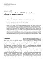
The extent of the neighbourhood depends on the chosen kernel function. Here, the first-
order, the second-order and the third-order B-spline functions with 8, 27 and 64 grid points
in neighbourhood for 3-D tasks or 4, 9 and 16 points in neighbourhood for 2-D tasks are
used. The particular choice of the kernel function affects the smoothness of the behaviour of
the regional similarity measure, see Fig. 5. The number of local optima is the lowest in the
case of the third-order B-spline. As the evaluation of the B-splines increases the
computational load, their values are computed only once and stored in a lookup table with
increments equal to 0.001.

Fig. 5. Comparison of the regional similarity measure computed with the use of GPV and
the first-order B-spline (solid line), the second-order B-spline (dashed line) and the third-
order B-spline (dotted line). A region of the size a) 10x10 mm, b) 20x20 mm was translated
by f
x
=±10mm in the x direction.

Local translations which maximize a matching criterion are searched in optimization
procedures. Here, the symmetric regional similarity measure is used as the matching
criterion which has to be maximized:


  






     
,,
,
WWWWW
reverse
W
WWWWW
forward
WWW

NMS
NMSS
fxuxx
xfxuxf



(16)

where f
W
=[f
1
, f
2
, , f
Kw
], f
1
=f
2
= f
Kw
=[f
x
, f
y
, f
z
]

T
is a translation of all voxels in a region W
along x, y and z axis. The use of the symmetric regional similarity measure and the GPV
interpolation with the use of the second-order B spline or the third order B-spline leads to
well-behaved criterion function in the case of large regions. In the case of small regions, the
uncertainty about the best translation is still high and many local maxima occur near the
optimal solution. A combination of extensive search and hillclimbing algorithms is used
here to find the global maximum. First, a space of all possible translations is determined by
absolute maximum translation |f
max
| in all directions. Then, the space of all possible
translations is searched with a relatively big step s
e
. The q best points are then used as
starting points for the following hillclimbing with a finer step s
h
. The maximum of q local
maxima obtained by the hillclimbing is then declared as the global maximum, see Fig. 6. All
the parameters of the optimization procedure depend on the size of the region which is
translated. In this way, fewer criterion evaluations are done for larger regions when the
chance of getting trapped into local maxima is reduced and more evaluations of the criterion
is performed for smaller regions.


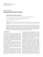
Fig. 6. A trajectory of 2-D optimization performed by an extensive search (triangles)
combined with hillclimbing (bold lines). The optimization procedure was set for this
illustration as follows: |f
max
|=[8, 8], s
e

=4 mm, s
h
=0.1 mm, q=8. The local maxima are marked
by crosses and the global one is marked by the circle.
Methods for Nonlinear Intersubject Registration in Neuroscience 59


Fig. 4. Illustration of regional symmetric matching. The similarity is measured in the
forward (the blue line) as well as in the reverse (the green line) direction of registration. In
the forward direction, the displacement field computed so far is applied on the floating
image voxels. In the reverse direction, the inverse displacement field is applied on the
reference image voxels.

The extent of the neighbourhood depends on the chosen kernel function. Here, the first-
order, the second-order and the third-order B-spline functions with 8, 27 and 64 grid points
in neighbourhood for 3-D tasks or 4, 9 and 16 points in neighbourhood for 2-D tasks are
used. The particular choice of the kernel function affects the smoothness of the behaviour of
the regional similarity measure, see Fig. 5. The number of local optima is the lowest in the
case of the third-order B-spline. As the evaluation of the B-splines increases the
computational load, their values are computed only once and stored in a lookup table with
increments equal to 0.001.


Fig. 5. Comparison of the regional similarity measure computed with the use of GPV and
the first-order B-spline (solid line), the second-order B-spline (dashed line) and the third-
order B-spline (dotted line). A region of the size a) 10x10 mm, b) 20x20 mm was translated
by f
x
=±10mm in the x direction.

Local translations which maximize a matching criterion are searched in optimization
procedures. Here, the symmetric regional similarity measure is used as the matching
criterion which has to be maximized:


  






     
,,
,
WWWWW
reverse
W
WWWWW
forward
WWW
NMS
NMSS
fxuxx
xfxuxf



(16)

where f
W
=[f
1
, f
2
, , f
Kw
], f
1
=f
2
= f
Kw
=[f
x
, f
y
, f
z
]
T
is a translation of all voxels in a region W
along x, y and z axis. The use of the symmetric regional similarity measure and the GPV
interpolation with the use of the second-order B spline or the third order B-spline leads to
well-behaved criterion function in the case of large regions. In the case of small regions, the
uncertainty about the best translation is still high and many local maxima occur near the
optimal solution. A combination of extensive search and hillclimbing algorithms is used
here to find the global maximum. First, a space of all possible translations is determined by
absolute maximum translation |f

max
| in all directions. Then, the space of all possible
translations is searched with a relatively big step s
e
. The q best points are then used as
starting points for the following hillclimbing with a finer step s
h
. The maximum of q local
maxima obtained by the hillclimbing is then declared as the global maximum, see Fig. 6. All
the parameters of the optimization procedure depend on the size of the region which is
translated. In this way, fewer criterion evaluations are done for larger regions when the
chance of getting trapped into local maxima is reduced and more evaluations of the criterion
is performed for smaller regions.


Fig. 6. A trajectory of 2-D optimization performed by an extensive search (triangles)
combined with hillclimbing (bold lines). The optimization procedure was set for this
illustration as follows: |f
max
|=[8, 8], s
e
=4 mm, s
h
=0.1 mm, q=8. The local maxima are marked
by crosses and the global one is marked by the circle.
Recent Advances in Signal Processing60

Image deformation based on interpolation with the use of RBFs is used here. The control
points p
i

are placed into the centers of the regions and their translations f
i
are obtained by
symmetric regional matching. Substituting the translations into (6), three systems of linear
equations are obtained and three vectors of w coefficients, where w is the number of the
regions, a
k
=(a
1,k
, , a
w,k
)
T
computed. The displacement of any point x is then defined
separately for each dimension by the interpolant:

 
 
.3 1,
1
,



kau
w
i
iCPkik
pxx


(17)

The values of spatial support s for various regions sizes are set empirically.
Optimal matches can be hardly found in a single pass composed of the local translations
estimation and the RBF-based interpolation, since features in one location influence
decisions at other locations of the images. Iterative updating scheme is therefore proposed
here. A multilevel strategy is incorporated into the proposed algorithm. The deformation is
iteratively refined in the coarse to fine manner. The size of the regions cannot be arbitrarily
small, because the local translations are determined independently for each region and
voxel interdependecies are introduced only by the regional similarity measure. The regions
containing poor contour or surface information can be eliminated from the matching process
and the algorithm can be accelerated in this way. The subdivision is performed only if at
least one voxel in the current region has its normalized gradient image intensity bigger then
a certain threshold.

3.2 High-dimensional deformable registration with the use of point similarity
measures and wavelet smoothing
The second registration algorithm produces high dimensional deformations involving gross
shape differences as well as local subtle differences between a subject and a template
anatomy. As multimodal similarity measures are used, the algorithm is suitable for DBM on
image data with different contrasts. There are two main parts repeated in an iterative
process as it was in the block matching algorithm: extraction of local forces f by
measurements of similarity and a spatial deformation model producing the displacement
field u. The main difference is that these parts are completely independent here, whereas the
regional similarity measure used in the block matching technique constrains the
deformation and thus it acts as a part of the spatial deformation model. Another difference
is in the way of extraction of the local forces. No local optimization is done here and the
forces are directly computed from the point similarity measures.
The registration algorithm is based on previous work and it differs from the one presented

in (Schwarz et al., 2007) namely in the spatial deformation model. The scheme of the
algorithm is in Fig. 7. The displacement field u which maximizes global mutual information
between a reference image and a floating image is searched in an iterative process which
involves computation of local forces f in each individual voxel x and their regularization by
the spatial deformation model. The regularization has two steps here. First, the
displacements proportional to forces are smoothed by wavelet thresholding. These
displacements are integrated into final deformation, which is done iteratively by
summation. The second part of the model represents behaviour of elastic materials where

displacements wane if the forces are retracted. This is ensured by the overall Gaussian
smoother.


Fig. 7. The scheme of the high-dimensional registration algorithm proposed for DBM. The
spatial deformation model consists of two basic components. First, the dense force field is
smoothed by wavelet thresholding and then the displacements are regularized by Gaussian
filtering to prevent breaking the topological condition of diffeomorphicity.

Methods for Nonlinear Intersubject Registration in Neuroscience 61

Image deformation based on interpolation with the use of RBFs is used here. The control
points p
i
are placed into the centers of the regions and their translations f
i
are obtained by
symmetric regional matching. Substituting the translations into (6), three systems of linear
equations are obtained and three vectors of w coefficients, where w is the number of the
regions, a
k

=(a
1,k
, , a
w,k
)
T
computed. The displacement of any point x is then defined
separately for each dimension by the interpolant:

 
 
.3 1,
1
,



kau
w
i
iCPkik
pxx


(17)

The values of spatial support s for various regions sizes are set empirically.
Optimal matches can be hardly found in a single pass composed of the local translations
estimation and the RBF-based interpolation, since features in one location influence
decisions at other locations of the images. Iterative updating scheme is therefore proposed

here. A multilevel strategy is incorporated into the proposed algorithm. The deformation is
iteratively refined in the coarse to fine manner. The size of the regions cannot be arbitrarily
small, because the local translations are determined independently for each region and
voxel interdependecies are introduced only by the regional similarity measure. The regions
containing poor contour or surface information can be eliminated from the matching process
and the algorithm can be accelerated in this way. The subdivision is performed only if at
least one voxel in the current region has its normalized gradient image intensity bigger then
a certain threshold.

3.2 High-dimensional deformable registration with the use of point similarity
measures and wavelet smoothing
The second registration algorithm produces high dimensional deformations involving gross
shape differences as well as local subtle differences between a subject and a template
anatomy. As multimodal similarity measures are used, the algorithm is suitable for DBM on
image data with different contrasts. There are two main parts repeated in an iterative
process as it was in the block matching algorithm: extraction of local forces f by
measurements of similarity and a spatial deformation model producing the displacement
field u. The main difference is that these parts are completely independent here, whereas the
regional similarity measure used in the block matching technique constrains the
deformation and thus it acts as a part of the spatial deformation model. Another difference
is in the way of extraction of the local forces. No local optimization is done here and the
forces are directly computed from the point similarity measures.
The registration algorithm is based on previous work and it differs from the one presented
in (Schwarz et al., 2007) namely in the spatial deformation model. The scheme of the
algorithm is in Fig. 7. The displacement field u which maximizes global mutual information
between a reference image and a floating image is searched in an iterative process which
involves computation of local forces f in each individual voxel x and their regularization by
the spatial deformation model. The regularization has two steps here. First, the
displacements proportional to forces are smoothed by wavelet thresholding. These
displacements are integrated into final deformation, which is done iteratively by

summation. The second part of the model represents behaviour of elastic materials where

displacements wane if the forces are retracted. This is ensured by the overall Gaussian
smoother.


Fig. 7. The scheme of the high-dimensional registration algorithm proposed for DBM. The
spatial deformation model consists of two basic components. First, the dense force field is
smoothed by wavelet thresholding and then the displacements are regularized by Gaussian
filtering to prevent breaking the topological condition of diffeomorphicity.

Recent Advances in Signal Processing62

Nearly symmetric orthogonal wavelet bases (Abdelnour & Selesnick, 2001) are used for the
decomposition and the reconstruction, which are performed in three levels here. All detail
coefficients in the first and in the second level of decomposition are set to zero in the
thresholding step of the algorithm. The initial setup of the standard deviation σ
G
of the
Gaussian filter is supposed to be found experimentally. The deformation has to preserve the
topology, i.e. one-to-one mappings termed as diffeomorphic should only be produced. This
requirement is satisfied if the determinant of the Jacobian of the deformation is held above
zero:

 
.)(,0det
333
222
111







































zyx
zyx
zyx




JJ

(18)

where φ
1
, φ
2
and φ
3
are components of the deformation over x, y and z axes respectively.
The values of the Jacobian determinant are estimated by symmetric finite differences. The
image is undesirably folded in the positions, where the Jacobian determinant is negative. In
such a case, the deformation is not invertible. The σ
G
-control block therefore ensures
increments in σ

G
if the minimum Jacobian determinant drops below a predefined threshold.
On the other hand, the deformation should capture subtle anatomical variations among
studied images. The σ
G
-control block therefore ensures decrements in σ
G
if the minimum
Jacobian determinant starts growing during the registration process.
Local forces are computed for each voxel independently as the difference between forward
forces and reverse forces, using the same symmetric registration approach as in the
previously described block-matching technique. The forces are estimated by the gradient of
a point similarity measure. The derivatives are approximated by central differences, such
that the k
th
component of a force at a voxel x is defined here as:

 




 
 
 
 
 
 
 
 

   
  
   
  
, 1,
2
,,
2
,,
Dk
ε
εNMSεNMS
ε
NεMSNεMS
fff
k
kk
k
kk
reverse
k
forward
kk








xuxxxuxx
xxuxxxux
xxx

(19)

where ε
k
is a voxel size component. The point similarity measure is evaluated in non-grid
positions due to the displacement field applied on the image grids. Thus, GPV interpolation
from neighboring grid points is employed here. For more details on computation and
normalization of the local forces see (Schwarz et al., 2007).


3.3 Evaluation of deformable registration methods
The quality of the presented registration algorithms is assessed here on recovering synthetic
deformations. The synthetic deformations based on thin-plate spline simulator (TPSsim) and
Rogelj’s spatial deformation simulator (RGsim) were applied to 2-D realistic T2-weighted
MRI images with 3% noise and 20% intensity nonuniformity from the Simulated Brain
Database (SBD) (Collins et al., 1998). The deformation simulators are described in detail in
(Schwarz et al., 2007). The deformed images were then registered to artifact-free T1-
weighted images from SBD and the error between the resulting and the initial deformation
was measured. The appropriate evaluation measures are the root mean-squared residual
displacement and the maximum absolute residual displacement. In the ideal case, the
composition of the resulting and initial deformation should give an identity transform with
no residual displacements.
Based on preliminary results and previous related works, the similarity measure S
PMI
was
used for both registration algorithms and the maximum level of subdivision in the block

matching technique was set to 5. This level corresponds to the subimage size of 7x7 pixels.
Although the next level of subdivision gave an increase in the global mutual information,
the alignment expressed by quantitative evaluation measures and also by visual inspection
was constant or worse.
The results expressed by root mean squared error displacements are presented
in Table 1 and Table 2. The high-dimensional deformable registration technique gives more
precise deformations with the respect to the lower residual error. The obtained results
showed its ability to recover the smooth deformations generated by TPSsim as well as the
complex deformations generated by RGsim.

|e
0
MAX
|

[mm]
e
0
RMS
[mm]

e
RMS
[mm]
o
1

o
2

o
1

o
2

o
1

o
2

o
1

o
2

o
1

o
2

o
1

o
2

1

1

2

1

3

1

2

2

3

2

3

3

TPSsim
5 2.47 0.59 0.57 0.56
0.51
0.52
0.51
8 3.95 0.74 0.71 0.69 0.68

0.67 0.67
10 4.93 0.91 0.89 0.86 0.85
0.82 0.82
12 5.92 1.17 1.38 1.34
1.16
1.36 1.35
RGsim
5 2.30 0.93 0.87 0.85 0.79 0.77
0.75
8 3.67 1.47 1.41 1.37 1.39 1.33
1.27
10 4.59 2.19 2.17 2.09 2.05 2.07
1.98
12 5.51 3.09 2.93
2.92
3.05 2.93 2.99
Table 1. Root mean squared error displacements achieved by the multilevel block matching
technique on various initial misregistration levels expressed by |e
0
MAX
|and e
0
RMS
and with
various setups in GPV interpolation kernel functions. The order of B-splines used in joint
PDF estimate construction is signed as o
1
and the order of B-splines used in regional
matching is signed as o
2

.


Methods for Nonlinear Intersubject Registration in Neuroscience 63

Nearly symmetric orthogonal wavelet bases (Abdelnour & Selesnick, 2001) are used for the
decomposition and the reconstruction, which are performed in three levels here. All detail
coefficients in the first and in the second level of decomposition are set to zero in the
thresholding step of the algorithm. The initial setup of the standard deviation σ
G
of the
Gaussian filter is supposed to be found experimentally. The deformation has to preserve the
topology, i.e. one-to-one mappings termed as diffeomorphic should only be produced. This
requirement is satisfied if the determinant of the Jacobian of the deformation is held above
zero:

 
.)(,0det
333
222
111






































zyx
zyx

zyx




JJ

(18)

where φ
1
, φ
2
and φ
3
are components of the deformation over x, y and z axes respectively.
The values of the Jacobian determinant are estimated by symmetric finite differences. The
image is undesirably folded in the positions, where the Jacobian determinant is negative. In
such a case, the deformation is not invertible. The σ
G
-control block therefore ensures
increments in σ
G
if the minimum Jacobian determinant drops below a predefined threshold.
On the other hand, the deformation should capture subtle anatomical variations among
studied images. The σ
G
-control block therefore ensures decrements in σ
G
if the minimum

Jacobian determinant starts growing during the registration process.
Local forces are computed for each voxel independently as the difference between forward
forces and reverse forces, using the same symmetric registration approach as in the
previously described block-matching technique. The forces are estimated by the gradient of
a point similarity measure. The derivatives are approximated by central differences, such
that the k
th
component of a force at a voxel x is defined here as:

 




 
 
 
 
 
 
 
 
   
  
   
  
, 1,
2
,,
2

,,
Dk
ε
εNMSεNMS
ε
NεMSNεMS
fff
k
kk
k
kk
reverse
k
forward
kk







xuxxxuxx
xxuxxxux
xxx

(19)

where ε
k

is a voxel size component. The point similarity measure is evaluated in non-grid
positions due to the displacement field applied on the image grids. Thus, GPV interpolation
from neighboring grid points is employed here. For more details on computation and
normalization of the local forces see (Schwarz et al., 2007).


3.3 Evaluation of deformable registration methods
The quality of the presented registration algorithms is assessed here on recovering synthetic
deformations. The synthetic deformations based on thin-plate spline simulator (TPSsim) and
Rogelj’s spatial deformation simulator (RGsim) were applied to 2-D realistic T2-weighted
MRI images with 3% noise and 20% intensity nonuniformity from the Simulated Brain
Database (SBD) (Collins et al., 1998). The deformation simulators are described in detail in
(Schwarz et al., 2007). The deformed images were then registered to artifact-free T1-
weighted images from SBD and the error between the resulting and the initial deformation
was measured. The appropriate evaluation measures are the root mean-squared residual
displacement and the maximum absolute residual displacement. In the ideal case, the
composition of the resulting and initial deformation should give an identity transform with
no residual displacements.
Based on preliminary results and previous related works, the similarity measure S
PMI
was
used for both registration algorithms and the maximum level of subdivision in the block
matching technique was set to 5. This level corresponds to the subimage size of 7x7 pixels.
Although the next level of subdivision gave an increase in the global mutual information,
the alignment expressed by quantitative evaluation measures and also by visual inspection
was constant or worse.
The results expressed by root mean squared error displacements are presented
in Table 1 and Table 2. The high-dimensional deformable registration technique gives more
precise deformations with the respect to the lower residual error. The obtained results
showed its ability to recover the smooth deformations generated by TPSsim as well as the

complex deformations generated by RGsim.

|e
0
MAX
|

[mm]
e
0
RMS
[mm]

e
RMS
[mm]
o
1

o
2

o
1

o
2

o
1

o
2

o
1

o
2

o
1

o
2

o
1

o
2

1 1 2 1 3 1 2 2 3 2 3 3
TPSsim
5 2.47 0.59 0.57 0.56
0.51
0.52
0.51
8 3.95 0.74 0.71 0.69 0.68
0.67 0.67

10 4.93 0.91 0.89 0.86 0.85
0.82 0.82
12 5.92 1.17 1.38 1.34
1.16
1.36 1.35
RGsim
5 2.30 0.93 0.87 0.85 0.79 0.77
0.75
8 3.67 1.47 1.41 1.37 1.39 1.33
1.27
10 4.59 2.19 2.17 2.09 2.05 2.07
1.98
12 5.51 3.09 2.93
2.92
3.05 2.93 2.99
Table 1. Root mean squared error displacements achieved by the multilevel block matching
technique on various initial misregistration levels expressed by |e
0
MAX
|and e
0
RMS
and with
various setups in GPV interpolation kernel functions. The order of B-splines used in joint
PDF estimate construction is signed as o
1
and the order of B-splines used in regional
matching is signed as o
2
.

Recent Advances in Signal Processing64

|e
0
MAX
|

[mm]
e
0
RMS
[mm]
e
RMS
[mm]
σ
G
=2.0 mm σ
G
=2.5 mm σ
G
=3.0 mm σ
G
=3.5 mm σ
G
=4.0 mm
RGsim
2.30 2.47 1.10 0.73

0.69
0.93 0.93
3.67 3.95 1.87
1.07
1.09 1.70 1.72
4.59 4.93 2.70
1.46
1.52 2.56 2.62
5.51 5.92 3.69
2.02
2.19 3.65 3.73
TPSsim
2.47 2.30 0.84 0.60
0.53
0.61 0.58
3.95 3.67 1.26 0.74
0.68
1.00 0.96
4.93 4.59 1.77 0.84
0.78
1.48 1.43
5.92 5.51 2.42 1.16
0.98
2.20 2.18
Table 2. Root mean squared error displacements achieved by the highdimensional
deformable registration method on various initial misregistration levels expressed by
|e
0
MAX
|and e

0
RMS
and with various setups in σ
G
. Highlighted values show the best results
achieved with the registration algorithm.

4. Deformation-based morphometry on real MRI datasets
In this section the results of high-resolution DBM in the first-episode and chronic
schizophrenia are presented, in order to demonstrate the ability of the high-dimensional
registration technique to capture the complex pattern of brain pathology in this condition.
High-resolution T1-weighted MRI brain scans of 192 male subjects were obtained with a
Siemens 1.5 T system in Faculty Hospital Brno. The group contained 49 male subjects with
first-episode schizophrenia (FES), 19 chronic schizophrenia subjects (CH) and 124 healthy
controls. The template from SBD which is based on 27 scans of one subject was used as the
reference anatomy and 192 template-to-subject registrations with the use of the presented
high-dimensional technique were performed. The resulting displacement vector fields were
converted into scalar fields by calculating Jacobian determinants in each voxel of the
stereotaxic space. The scalar fields were put into statistical analysis which included
assessing normality, parametric significance testing. The Jacobian determinant can be
viewed as a parameter which characterizes local volume changes, i.e. local shrinkage or
enlargement caused by a deformation. The analysis of the scalar fields produced spatial map
of t statistic which allowed to localize regions with significant differences in volumes of
anatomical structures between the groups. Complex patterns of brain anatomy changes in
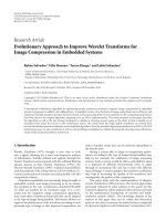
schizophrenia subjects as compared to healthy controls were detected, see Fig. 8.



Fig. 8. Selected slices of t statistic overlaid over the SBD template. The t values were
thresholded at the levels of significance


=5% corrected for multiple testing by the False
Detection Rate method. The yellow regions represent local volume reductions in
schizophrenia subjects compared to healthy controls and the red regions represent local
volume enlargements. Compared groups: a) FES
CH vs. NC, b) FES vs. NC, c) CH vs. NC.

5. Conclusion
In this chapter two deformable registration methods were described: 1) a block matching
technique based on parametric transformations with radial basis functions
and 2) a high-dimensional registration technique with nonparametric deformation models
based on spatial smoothing. The use of multimodal similarity measures was insisted. The
multimodal character of the methods make them robust to tissue intensity variations which
can be result of multimodality imaging as well as neuropsychological diseases or even
normal aging.
One of the described algorithms was demonstrated in the field of computational
neuroanatomy, particularly for fully automated spatial detection of anatomical
abnormalities in first-episode and chronic schizophrenia based on 3-D MRI brain scans.

Acknowledgement
The work was supported by grants IGA MH CZ NR No. 9893-4 and No. 10347-3.

Methods for Nonlinear Intersubject Registration in Neuroscience 65

|e
0
MAX
|

[mm]

e
0
RMS
[mm]
e
RMS
[mm]
σ
G
=2.0 mm σ
G
=2.5 mm σ
G
=3.0 mm σ
G
=3.5 mm σ
G
=4.0 mm
RGsim
2.30 2.47 1.10 0.73
0.69
0.93 0.93
3.67 3.95 1.87
1.07
1.09 1.70 1.72
4.59 4.93 2.70
1.46
1.52 2.56 2.62
5.51 5.92 3.69
2.02

2.19 3.65 3.73
TPSsim
2.47 2.30 0.84 0.60
0.53
0.61 0.58
3.95 3.67 1.26 0.74
0.68
1.00 0.96
4.93 4.59 1.77 0.84
0.78
1.48 1.43
5.92 5.51 2.42 1.16
0.98
2.20 2.18
Table 2. Root mean squared error displacements achieved by the highdimensional
deformable registration method on various initial misregistration levels expressed by
|e
0
MAX
|and e
0
RMS
and with various setups in σ
G
. Highlighted values show the best results
achieved with the registration algorithm.

4. Deformation-based morphometry on real MRI datasets
In this section the results of high-resolution DBM in the first-episode and chronic
schizophrenia are presented, in order to demonstrate the ability of the high-dimensional

registration technique to capture the complex pattern of brain pathology in this condition.
High-resolution T1-weighted MRI brain scans of 192 male subjects were obtained with a
Siemens 1.5 T system in Faculty Hospital Brno. The group contained 49 male subjects with
first-episode schizophrenia (FES), 19 chronic schizophrenia subjects (CH) and 124 healthy
controls. The template from SBD which is based on 27 scans of one subject was used as the
reference anatomy and 192 template-to-subject registrations with the use of the presented
high-dimensional technique were performed. The resulting displacement vector fields were
converted into scalar fields by calculating Jacobian determinants in each voxel of the
stereotaxic space. The scalar fields were put into statistical analysis which included
assessing normality, parametric significance testing. The Jacobian determinant can be
viewed as a parameter which characterizes local volume changes, i.e. local shrinkage or
enlargement caused by a deformation. The analysis of the scalar fields produced spatial map
of t statistic which allowed to localize regions with significant differences in volumes of
anatomical structures between the groups. Complex patterns of brain anatomy changes in
schizophrenia subjects as compared to healthy controls were detected, see Fig. 8.



Fig. 8. Selected slices of t statistic overlaid over the SBD template. The t values were
thresholded at the levels of significance

=5% corrected for multiple testing by the False
Detection Rate method. The yellow regions represent local volume reductions in
schizophrenia subjects compared to healthy controls and the red regions represent local
volume enlargements. Compared groups: a) FES
CH vs. NC, b) FES vs. NC, c) CH vs. NC.

5. Conclusion
In this chapter two deformable registration methods were described: 1) a block matching
technique based on parametric transformations with radial basis functions

and 2) a high-dimensional registration technique with nonparametric deformation models
based on spatial smoothing. The use of multimodal similarity measures was insisted. The
multimodal character of the methods make them robust to tissue intensity variations which
can be result of multimodality imaging as well as neuropsychological diseases or even
normal aging.
One of the described algorithms was demonstrated in the field of computational
neuroanatomy, particularly for fully automated spatial detection of anatomical
abnormalities in first-episode and chronic schizophrenia based on 3-D MRI brain scans.

Acknowledgement
The work was supported by grants IGA MH CZ NR No. 9893-4 and No. 10347-3.

Recent Advances in Signal Processing66

References
Abdelnour, A. F. & Selesnick, I. W. (2001). Nearly symmetric orthogonal wavelet bases. Proc.
IEEE Int. Conf. Acoust., Speech, Signal Processing (ICASSP), May 2001, IEEE,
Salt Lake City
Ali, A. A.; Dale, A. M.; Badea, A. & Johnson, G. A. (2005). Automated segmentation of
neuroanatomical structures in multispectral MR microscopy of the mouse brain.
NeuroImage, Vol. 27, No. 2, 425–435, ISSN 1053-8119
Alterovitz, R.; Goldberg, K.; Kurhanewicz, J.; Pouliot, J. & Hsu, I. (2004). Image registration
for prostate MR spectroscopy using biomechanical modeling and optimization of
force and stiffness parameters. Proceedings of 26th Annual International Conference of
IEEE Engineering in Medicine and Biology Society, 2004, pp. 1722–1725,
ISBN 0-7803-8440-7, IEEE, San Francisco
Amidror, I. (2002). Scattered data interpolation methods for electronic imaging systems: a
survey. Journal of Electronic Imaging, Vol. 11, No. 2, pp.157–176, ISSN 1017-9909
Ashburner, J. & Friston, K. J. (2000). Voxel-based morphometry – the methods. NeuroImage,
Vol. 11, No. 6, 805–821, ISSN 1053-8119

Ashburner, J. (2007). A fast diffeomorphic image registration algorithm. NeuroImage, Vol. 38,
No. 1, 95–113, ISSN 1053-8119
Chen, H. & Varshney, P. K. (2003). Mutual information-based CT-MR brain image
registration using generalized partial volume point histogram estimation. IEEE
Transactions on Medical Imaging, Vol. 22, No. 9, 1111–1119, ISSN 0278-0062
Christensen, G. E.; Rabbitt, R. D. & Miller M. I. (1996). Deformable templates using large
deformation kinematics. IEEE Transactions on Image Processing, Vol. 5, No. 10, 1435–
1447, ISSN 0278-0062.
Clatz, O. et al. (2005). Robust nonrigid registration to capture brain shift from intraoperative
MRI. IEEE Transactions on Medical Imaging, Vol. 24, No. 11, 1417–1427,
ISSN 0278-0062.
Collins, D. L. et al. (1998). Design and construction of a realistic digital brain phantom.IEEE
Transactions on Medical Imaging, Vol. 17, No. 3, 463–468, ISSN 0278-0062
Collins, D. L.; Neelin, P.; Peters, T. M. & Evans, A. C. (1994). Automatic 3D inter-subject
registration of MR volumetric data in standardized Talairach space. Journal of
Computer Assisted Tomography, Vol. 18, No. 2, 192–205, ISSN 0363-8715.
Čapek, M.; Mroz, L. & Wegenkittl, R. (2001). Robust and fast medical registration of 3D-
multi-modality data sets. Proceedings of the International Federation for Medical &
Biological Engineering, pp. 515–518, ISBN 953-184-023-7, Pula
Donato, G. & Belongie, S. (2002). Approximation methods for thin plate spline mappings
and principal warps. Proceedings of European Conference on Computer Vision,
pp. 531–542
Downie, T. R. & Silverman, B. W. (2001). A wavelet mixture approach to the estimation of
image deformation functions. Sankhya: The Indian Journal Of Statistics Series B,
Vol. 63, No. 2, 181–198, ISSN 0581-5738
Ferrant, M.; Warfield, S. K.; Nabavi, A.; Jolesz, F. A. & Kikinis, R. (2001). Registration of 3D
intraoperative MR images of the brain using a finite element biomechanical model.
In: IEEE Transactions on Medical Imaging, Vol. 20, No. 12, 1384–97, ISSN 0278-0062

Fornefett, M.; Rohr, K. & Stiehl, H. S. (2001). Radial basis functions with compact support for

elastic registration of medical images. Image and Vision Computing, Vol. 19, No. 1,
87–96, ISSN 0262-8856
Friston, K. J. et al. (2007). Statistical Parametric Mapping: The Analysis of Functional Brain
Images, Elsevier, ISBN 0123725607, London
Gaser, C. et al. (2001). Deformation-based morphometry and its relation to conventional
volumetry of brain lateral ventricles in MRI. NeuroImage, Vol. 13, No. 6, 1140–1145,
ISSN 1053-8119
Gaser, C. et al. (2004). Ventricular enlargement in schizophrenia related to volume reduction
of the thalamus, striatum, and superior temporal cortex. American Journal of
Psychiatry, Vol. 161, No. 1, 154–156, ISSN 0002-953X
Gholipour, A. et al. (2007). Brain functional localization: a survey of image registration
techniques. IEEE Transactions on Medical Imaging, Vol. 26, No. 4, 427–451,
ISSN 0278-0062.
Gramkow, C. & Bro-Nielsen, M. (1997). Comparison of three filters in the solution of the
Navier-Stokes equation in registration. Proceedings of Scandinavian Conference on
Image Analysis SCIA'97, 1997, pp. 795–802, Lappeenranta
Ibanez, L.; Schroeder, W.; Ng, L. & Cates, J. (2003). The ITK Software Guide. Kitware Inc,
ISBN 1930934106
Kostelec, P.; Weaver, J. & Healy D. Jr. (1998). Multiresolution elastic image registration.
Medical Physics, Vol. 25, No. 9, 1593–1604, ISSN 0094-2405
Kubečka, L. & Jan, J. (2004). Registration of bimodal retinal images - improving
modifications. Proceedings of 26th Annual International Conference of IEEE Engineering
in Medicine and Biology Society, pp. 1695–1698, ISBN 0-7803-8440-7, IEEE,
San Francisco
Maes, F. (1998). Segmentation and registration of multimodal medical images: from theory,
implementation and validation to a useful tool in clinical practice. Catholic
University, Leuven
Maintz, J. B. A. & Viergever, M. A. (1998). A survey of medical image registration. Medical
Image Analysis, Vol. 2, No. 1, 1–37, ISSN 1361-8415
Maintz, J. B. A.; Meijering, E. H. W. & Viergever, M. A. (1998). General multimodal elastic

registration based on mutual Information. In: Medical Imaging 1998: Image
Processing, Kenneth, M. & Hanson, (Ed.), 144–154, SPIE
Mechelli, A., Price, C. J., Friston, K. J. & Ashburner, J. (2005). Voxel-based morphometry of
the human brain: methods and applications. Current Medical Imaging Reviews, vol. 1,
No. 2, 105–113, ISSN 1573-4056
Modersitzki, J. (2004). Numerical Methods for Image Registration. Oxford University Press,
ISBN 0198528418, New York.
Pauchard, Y.; Smith, M. R. & Mintchev, M. P. (2004). Modeling susceptibility difference
artifacts produced by metallic implants in magnetic resonance imaging with point-
based thin-plate spline image registration. Proceedings of 26th Annual International
Conference of IEEE Engineering in Medicine and Biology Society, pp. 1766–1769,
ISBN 0-7803-8440-7, IEEE, San Francisco
Peckar, W.; Schnörr, C.; Rohr, K.; Stiehl, H. S. & Spetzger, U. (1998). Linear and incremental
estimation of elastic deformations in medical registration using prescribed
displacements. Machine Graphics & Vision, Vol. 7, No. 4, 807–829, ISSN 1230-0535
Methods for Nonlinear Intersubject Registration in Neuroscience 67

References
Abdelnour, A. F. & Selesnick, I. W. (2001). Nearly symmetric orthogonal wavelet bases. Proc.
IEEE Int. Conf. Acoust., Speech, Signal Processing (ICASSP), May 2001, IEEE,
Salt Lake City
Ali, A. A.; Dale, A. M.; Badea, A. & Johnson, G. A. (2005). Automated segmentation of
neuroanatomical structures in multispectral MR microscopy of the mouse brain.
NeuroImage, Vol. 27, No. 2, 425–435, ISSN 1053-8119
Alterovitz, R.; Goldberg, K.; Kurhanewicz, J.; Pouliot, J. & Hsu, I. (2004). Image registration
for prostate MR spectroscopy using biomechanical modeling and optimization of
force and stiffness parameters. Proceedings of 26th Annual International Conference of
IEEE Engineering in Medicine and Biology Society, 2004, pp. 1722–1725,
ISBN 0-7803-8440-7, IEEE, San Francisco
Amidror, I. (2002). Scattered data interpolation methods for electronic imaging systems: a

survey. Journal of Electronic Imaging, Vol. 11, No. 2, pp.157–176, ISSN 1017-9909
Ashburner, J. & Friston, K. J. (2000). Voxel-based morphometry – the methods. NeuroImage,
Vol. 11, No. 6, 805–821, ISSN 1053-8119
Ashburner, J. (2007). A fast diffeomorphic image registration algorithm. NeuroImage, Vol. 38,
No. 1, 95–113, ISSN 1053-8119
Chen, H. & Varshney, P. K. (2003). Mutual information-based CT-MR brain image
registration using generalized partial volume point histogram estimation. IEEE
Transactions on Medical Imaging, Vol. 22, No. 9, 1111–1119, ISSN 0278-0062
Christensen, G. E.; Rabbitt, R. D. & Miller M. I. (1996). Deformable templates using large
deformation kinematics. IEEE Transactions on Image Processing, Vol. 5, No. 10, 1435–
1447, ISSN 0278-0062.
Clatz, O. et al. (2005). Robust nonrigid registration to capture brain shift from intraoperative
MRI. IEEE Transactions on Medical Imaging, Vol. 24, No. 11, 1417–1427,
ISSN 0278-0062.
Collins, D. L. et al. (1998). Design and construction of a realistic digital brain phantom.IEEE
Transactions on Medical Imaging, Vol. 17, No. 3, 463–468, ISSN 0278-0062
Collins, D. L.; Neelin, P.; Peters, T. M. & Evans, A. C. (1994). Automatic 3D inter-subject
registration of MR volumetric data in standardized Talairach space. Journal of
Computer Assisted Tomography, Vol. 18, No. 2, 192–205, ISSN 0363-8715.
Čapek, M.; Mroz, L. & Wegenkittl, R. (2001). Robust and fast medical registration of 3D-
multi-modality data sets. Proceedings of the International Federation for Medical &
Biological Engineering, pp. 515–518, ISBN 953-184-023-7, Pula
Donato, G. & Belongie, S. (2002). Approximation methods for thin plate spline mappings
and principal warps. Proceedings of European Conference on Computer Vision,
pp. 531–542
Downie, T. R. & Silverman, B. W. (2001). A wavelet mixture approach to the estimation of
image deformation functions. Sankhya: The Indian Journal Of Statistics Series B,
Vol. 63, No. 2, 181–198, ISSN 0581-5738
Ferrant, M.; Warfield, S. K.; Nabavi, A.; Jolesz, F. A. & Kikinis, R. (2001). Registration of 3D
intraoperative MR images of the brain using a finite element biomechanical model.

In: IEEE Transactions on Medical Imaging, Vol. 20, No. 12, 1384–97, ISSN 0278-0062

Fornefett, M.; Rohr, K. & Stiehl, H. S. (2001). Radial basis functions with compact support for
elastic registration of medical images. Image and Vision Computing, Vol. 19, No. 1,
87–96, ISSN 0262-8856
Friston, K. J. et al. (2007). Statistical Parametric Mapping: The Analysis of Functional Brain
Images, Elsevier, ISBN 0123725607, London
Gaser, C. et al. (2001). Deformation-based morphometry and its relation to conventional
volumetry of brain lateral ventricles in MRI. NeuroImage, Vol. 13, No. 6, 1140–1145,
ISSN 1053-8119
Gaser, C. et al. (2004). Ventricular enlargement in schizophrenia related to volume reduction
of the thalamus, striatum, and superior temporal cortex. American Journal of
Psychiatry, Vol. 161, No. 1, 154–156, ISSN 0002-953X
Gholipour, A. et al. (2007). Brain functional localization: a survey of image registration
techniques. IEEE Transactions on Medical Imaging, Vol. 26, No. 4, 427–451,
ISSN 0278-0062.
Gramkow, C. & Bro-Nielsen, M. (1997). Comparison of three filters in the solution of the
Navier-Stokes equation in registration. Proceedings of Scandinavian Conference on
Image Analysis SCIA'97, 1997, pp. 795–802, Lappeenranta
Ibanez, L.; Schroeder, W.; Ng, L. & Cates, J. (2003). The ITK Software Guide. Kitware Inc,
ISBN 1930934106
Kostelec, P.; Weaver, J. & Healy D. Jr. (1998). Multiresolution elastic image registration.
Medical Physics, Vol. 25, No. 9, 1593–1604, ISSN 0094-2405
Kubečka, L. & Jan, J. (2004). Registration of bimodal retinal images - improving
modifications. Proceedings of 26th Annual International Conference of IEEE Engineering
in Medicine and Biology Society, pp. 1695–1698, ISBN 0-7803-8440-7, IEEE,
San Francisco
Maes, F. (1998). Segmentation and registration of multimodal medical images: from theory,
implementation and validation to a useful tool in clinical practice. Catholic
University, Leuven

Maintz, J. B. A. & Viergever, M. A. (1998). A survey of medical image registration. Medical
Image Analysis, Vol. 2, No. 1, 1–37, ISSN 1361-8415
Maintz, J. B. A.; Meijering, E. H. W. & Viergever, M. A. (1998). General multimodal elastic
registration based on mutual Information. In: Medical Imaging 1998: Image
Processing, Kenneth, M. & Hanson, (Ed.), 144–154, SPIE
Mechelli, A., Price, C. J., Friston, K. J. & Ashburner, J. (2005). Voxel-based morphometry of
the human brain: methods and applications. Current Medical Imaging Reviews, vol. 1,
No. 2, 105–113, ISSN 1573-4056
Modersitzki, J. (2004). Numerical Methods for Image Registration. Oxford University Press,
ISBN 0198528418, New York.
Pauchard, Y.; Smith, M. R. & Mintchev, M. P. (2004). Modeling susceptibility difference
artifacts produced by metallic implants in magnetic resonance imaging with point-
based thin-plate spline image registration. Proceedings of 26th Annual International
Conference of IEEE Engineering in Medicine and Biology Society, pp. 1766–1769,
ISBN 0-7803-8440-7, IEEE, San Francisco
Peckar, W.; Schnörr, C.; Rohr, K.; Stiehl, H. S. & Spetzger, U. (1998). Linear and incremental
estimation of elastic deformations in medical registration using prescribed
displacements. Machine Graphics & Vision, Vol. 7, No. 4, 807–829, ISSN 1230-0535
Recent Advances in Signal Processing68

Pluim, P. W. J.; Maintz J. B. A. & Viergever M. A. (2001). Mutual information matching in
multiresolution contexts. Image and Vision Computing, Vol. 19, No. 1, 45–52,
ISSN 0262-8856
Rogelj, P.; Kovačič, S. & Gee, J. C. (2003). Point similarity measures for non-rigid registration
of multi-modal data. Computer Vision and Image Understanding, Vol. 92, No. 1,
112–140, ISSN 1077-3142
Rogelj, P. & Kovačič, S. (2003). Point similarity measure based on mutual information. In:
Biomedical Image Registration: Revised Papers, Gee, J. C.; Maintz, J. B. A. & Vannier,
M. W. (Ed.), 112–121, Springer-Verlag, ISBN 978-3-540-20343-8
Rogelj, P. & Kovačič, S. (2003). Symmetric image registration. Medical Image Analysis, Vol. 10,

No. 3, 484–493, ISSN 1361-8415
Rogelj, P. & Kovačič, S. (2004). Spatial deformation models for non-rigid image registration.
Proceedings of 9th Computer Vision Winter Workshop CVWW'04, 2004, pp. 79–88,
Slovenian Pattern Recognition Society, Piran.
Rohlfing, T.; Maurer, C. R.; Bluemke, D. A. & Jacobs, M. A. (2003). Volume-preserving
nonrigid registration of MR breast images using free-form deformation with an
incompresibility constraint. IEEE Transactions on Medical Imaging, Vol. 12, No. 6,
730–741, ISSN 0278-0062.
Rohr, K. (2001). Elastic registration of multimodal medical images: a survey. Künstliche
Intelligenz, Vol. 14, No. 3, 11–17, ISSN 0933-1875
Rueckert, D. et al. (1999). Nonrigid registration using free-form deformations: application to
breast MR images. IEEE Transactions on Medical Imaging, Vol. 18, No. 8, 712–721,
ISSN 0278-0062
Schnabel, J. A. et al. (2003). Validation of non-rigid image registration using finite element
methods: application to breast MR images. IEEE Transactions on Medical Imaging,
Vol. 22, No. 2, 238–247, ISSN 0278-0062.
Schwarz, D.; Kašpárek, T., Provazník, I. & Jarkovský, J. (2007). A deformable registration
method for automated morphometry of MRI brain images in neuropsychiatric
research. IEEE Transactions on Medical Imaging, Vol. 26, No. 4, 452-461,
ISSN 0278-0062.
Studholme, C.; Hill, D. L. G.; & Hawkes, D. J. (1999). An overlap invariant entropy measure
of 3D medical image alignment. Pattern Recognition, Vol. 32, No. 1, 71–86,
ISSN 1054-6618
Thirion, J. P. (1998). Image matching as a diffusion process: an analogy with Maxwell’s
demons. Medical Image Analysis, Vol. 2, No. 3, 243–260, ISSN 1361-8415
Viola, P. & Wells, W. M. (1995). Alignment by maximization of mutual information.
International Journal of Computer Vision, Vol. 24, No. 2, 137–154, ISSN 0920-5691
Wendland, H. (1995). Piecewise polynomial, positive definite and compactly supported
radial functions of minimal degree. Advances in Computational Mathematics, Vol. 4,
No. 1, 389–396, ISSN 1019-7168

Xu, L.; Groth, K. M.; Pearlson, G.; Schretlen, D. J.; Calhoun, V. D. (2008). Source-based
morphometry: the use of independent component analysis to identify gray matter
differences with application to schizophrenia. Human Brain Mapping, Vol. 30, No. 3,
711–724, ISSN 1065-9471
Zitova, B. and Flusser J. (2003). Image registration methods: a survey. Image and Vision
Computing, Vol. 21, No. 11, 977–1000, ISSN 0262-8856
Functional semi-automated segmentation of renal
DCE-MRI sequences using a Growing Neural Gas algorithm 69
Functional semi-automated segmentation of renal DCE-MRI sequences
using a Growing Neural Gas algorithm
Chevaillier Beatrice, Collette Jean-Luc, Mandry Damien and Claudon
X

Functional semi-automated segmentation of
renal DCE-MRI sequences using a Growing
Neural Gas algorithm

Chevaillier Beatrice
(1)
, Collette Jean-Luc
(1)
, Mandry Damien
(2)
, Claudon
Michel
(2)
& Pietquin Olivier
(1,2)

(1)
SUPELEC-Metz campus, IMS Research Group

(2)
IADI, INSERM, ERI 13 ; Nancy University
France

1. Introduction

In this chapter we describe a semi-automatic segmentation method for dynamic contrast-
enhanced magnetic resonance imaging (DCE-MRI) sequences for renal function assessment.
Among the different MRI techniques aiming at studying the renal function, DCE-MRI with
gadolinium chelates injection is the most widely used (Grenier et al., 2003). Several
parameters like the glomerular filtration rate or the differential renal function can be non-
invasively computed from perfusion curves of different Regions Of Interest (ROI). So
segmentation of internal anatomical kidney structures like cortex, medulla and pelvo-
caliceal cavities is crucial for functional assessment detection of diseases affecting different
parts of this organ. Manual segmentation by a radiologist is fairly delicate because images
are blurred and highly noisy. Moreover the different compartments are not visible during
the same perfusion phase because of contrast changes: cavities are enhanced during late
perfusion phase, whereas cortex and medulla can only be separated near the cortical peak,
when the contrast agent enters the kidney (figure 1); consequently they cannot be delineated
on a single image. Radiologists have to examine the whole sequence in order to choose the
two most suitable frames: the operation is time-consuming and functional analysis can vary
greatly in case of misregistration or through-plane motion. Some classical semi-automated
methods are often used in the medical field but few of them have been tested on renal DCE-
MRI sequences (Michoux et al., 2006). In (Coulam et al., 2002), cortex of pig kidneys is
delineated by simple intensity thresholding during cortical enhancement phase, but
precision is limited essentially because of noise. In (Lv et al., 2008), a three-dimensional
kidney extraction and a segmentation of internal renal structures are performed using a

region-growing technique. Anyway only few frames are used, so problems due frames
selection and non corrected motion remain. As the contrast temporal evolution is different
in every compartment for physiological reasons, pixels can be classified according to their
time-intensity curves: such a method can improve both noise robustness and
reproducibility. In (Zoellner et al., 2006), independent component analysis allows recovering
5
Recent Advances in Signal Processing70

some functional regions but does not result in segmentations comparable to morphological
ones: any pixel can actually be attributed to zero, one or more compartment. In (Sun et al.,
2004), a multi-step approach including successive registrations and segmentations is
proposed: pixels are classified using a K-means partitioning algorithm applied to their time-
intensity curves. Nevertheless a functional segmentation using some unsupervised
classification method and resulting in only three ROIs corresponding to cortex, medulla and
cavities seems to be hard to obtained directly. This is mainly due to considerable contrast
dissimilarities between pixels in a same compartment despite some common characteristics
(Chevaillier et al., 2008a).
Concerning validation, very few results for real data have been exposed. In (Rusinek et al.,
2007), a segmentation error is defined in connection with a manual segmentation as the
global volume of false-positive (oversegmented) and false-negative (undersegmented)
voxels. Nevertheless assessment consists mostly in qualitative consistency with manual
segmentations or in comparisons between the corresponding compartment volumes or
between the induced renograms (Song et al., 2005).

We propose to test a semi-automated split (2.1) and merge method (2.2) for renal functional
segmentation. The kidney pixels are first clustered according to their contrast evolution
using a vector quantization algorithm. These clusters are then merged thanks to some
characteristic criteria of their prototype functional curves to get the three final anatomical
compartments. Operator intervention consists only in a coarse tuning of two independent
thresholds for merging, and is thus easy and quick to perform while keeping the

practitioner into the loop. The method is also relatively robust because the whole sequence
is used instead of only two frames as for traditional manual segmentation. In the absence of
ground truth for results assessment, a manual anatomical segmentation by a radiologist is
considered as a reference. Some discrepancy criteria are computed between this
segmentation and functional ones. As a comparison, the same criteria are evaluated between
the reference and another manual segmentation.
This book chapter is an extended version of (Chevaillier et al., 2008b).

2. Method for functional segmentation

2.1 Vector quantization of time-intensity curves
The temporal evolution of contrast for each of the
N pixels of a kidney results from a DCE-
MRI registered sequence: examples of three frames for different perfusion phases can be
seen in figure 1.
Let
ip
I
be the intensity at time p for the pixel
i
x ,
B
I the mean value for baseline and
L
I
the mean value during late phase for the time-intensity curve of entire kidney. Let


T
iNii


, ,
1

be the
T
N -components vector associated with each pixel, where


 
BLBipip
IIII  /

(intensity normalization is performed in order to have similar
dynamic for any kidney). The
N vectors
i

are considered as samples of an unknown
probability distribution over a manifold
T
N
RX  with a density of probability
 

p .


Fig. 1.
Examples of frames from a DCE-MRI sequence during arterial peak (left), filtration

(middle) and late phase (right)

The aim is to find a set


Xw
Kj
j

1
of prototypes (or nodes) that maps the distribution
with a given distortion. Let be
 
2
minarg
jw
ww
j


. The Growing Neural Gas with
targeting (GNG-T) (Frezza-Buet, 2008), which is a variant of the classical Growing Neural
Gas algorithm (Fritzke, 1995), minimizes a cost function that tends towards the distortion:
   




K
j

j
X
EdpwE
1
2
(


(1)
where
 

dpwE
j
V
jj
2

 and




jj
wwXV 

:

(2)
j

V is the so-called Voronoï cell of
j
w and consists of all points of
X
that are closer to
j
w
than to any other
i
w . The set of


Kj
j
V
1
is a partition of
X
.
More precisely, GNG-T algorithm builds iteratively a network consisting in both:
 a set of prototypes,
 a graph structure preserving the topology of the underlying probability
distribution.
This graph is made up of a set of connections between nodes defining a topological
neighbourhood relation in the parameter space. It approximates the induced Delaunay
triangulation of the set


Kj
j

w
1
on the manifold
X
(Martinetz et al., 1993). Edges are
drawn up according to a competitive Hebbian learning rule: the basic principle is, for each
input
i

, to connect the two best matching prototypes. Two prototypes that are directly
Functional semi-automated segmentation of renal
DCE-MRI sequences using a Growing Neural Gas algorithm 71

some functional regions but does not result in segmentations comparable to morphological
ones: any pixel can actually be attributed to zero, one or more compartment. In (Sun et al.,
2004), a multi-step approach including successive registrations and segmentations is
proposed: pixels are classified using a K-means partitioning algorithm applied to their time-
intensity curves. Nevertheless a functional segmentation using some unsupervised
classification method and resulting in only three ROIs corresponding to cortex, medulla and
cavities seems to be hard to obtained directly. This is mainly due to considerable contrast
dissimilarities between pixels in a same compartment despite some common characteristics
(Chevaillier et al., 2008a).
Concerning validation, very few results for real data have been exposed. In (Rusinek et al.,
2007), a segmentation error is defined in connection with a manual segmentation as the
global volume of false-positive (oversegmented) and false-negative (undersegmented)
voxels. Nevertheless assessment consists mostly in qualitative consistency with manual
segmentations or in comparisons between the corresponding compartment volumes or
between the induced renograms (Song et al., 2005).

We propose to test a semi-automated split (2.1) and merge method (2.2) for renal functional

segmentation. The kidney pixels are first clustered according to their contrast evolution
using a vector quantization algorithm. These clusters are then merged thanks to some
characteristic criteria of their prototype functional curves to get the three final anatomical
compartments. Operator intervention consists only in a coarse tuning of two independent
thresholds for merging, and is thus easy and quick to perform while keeping the
practitioner into the loop. The method is also relatively robust because the whole sequence
is used instead of only two frames as for traditional manual segmentation. In the absence of
ground truth for results assessment, a manual anatomical segmentation by a radiologist is
considered as a reference. Some discrepancy criteria are computed between this
segmentation and functional ones. As a comparison, the same criteria are evaluated between
the reference and another manual segmentation.
This book chapter is an extended version of (Chevaillier et al., 2008b).

2. Method for functional segmentation

2.1 Vector quantization of time-intensity curves
The temporal evolution of contrast for each of the
N pixels of a kidney results from a DCE-
MRI registered sequence: examples of three frames for different perfusion phases can be
seen in figure 1.
Let
ip
I
be the intensity at time p for the pixel
i
x ,
B
I the mean value for baseline and
L
I

the mean value during late phase for the time-intensity curve of entire kidney. Let


T
iNii

, ,
1

be the
T
N -components vector associated with each pixel, where


 
BLBipip
IIII

 /

(intensity normalization is performed in order to have similar
dynamic for any kidney). The
N vectors
i

are considered as samples of an unknown
probability distribution over a manifold
T
N
RX  with a density of probability

 

p .


Fig. 1.
Examples of frames from a DCE-MRI sequence during arterial peak (left), filtration
(middle) and late phase (right)

The aim is to find a set


Xw
Kj
j

1
of prototypes (or nodes) that maps the distribution
with a given distortion. Let be
 
2
minarg
jw
ww
j


. The Growing Neural Gas with
targeting (GNG-T) (Frezza-Buet, 2008), which is a variant of the classical Growing Neural
Gas algorithm (Fritzke, 1995), minimizes a cost function that tends towards the distortion:

   




K
j
j
X
EdpwE
1
2
(


(1)
where
 

dpwE
j
V
jj
2

 and





jj
wwXV 

:

(2)
j
V is the so-called Voronoï cell of
j
w and consists of all points of
X
that are closer to
j
w
than to any other
i
w . The set of


Kj
j
V
1
is a partition of
X
.
More precisely, GNG-T algorithm builds iteratively a network consisting in both:
 a set of prototypes,
 a graph structure preserving the topology of the underlying probability
distribution.

This graph is made up of a set of connections between nodes defining a topological
neighbourhood relation in the parameter space. It approximates the induced Delaunay
triangulation of the set


Kj
j
w
1
on the manifold
X
(Martinetz et al., 1993). Edges are
drawn up according to a competitive Hebbian learning rule: the basic principle is, for each
input
i

, to connect the two best matching prototypes. Two prototypes that are directly
Recent Advances in Signal Processing72

linked in the final graph should thus have similar temporal behaviour. Both the winner, i.e.
the closest prototype of the current data point, and all its topological neighbours are
adjusted after each iteration. Influence of initialization is thus reduced for GNG-T compared
to on-line K-means for instance.
The number
K
of prototypes is iteratively determined to reach a given average node
distortion
T
. While a prior lattice has to be chosen for other algorithms like self-organising
map (Kohonen, 2001), no topological knowledge is required here: the graph adapts

automatically to any distribution structure during the building process.
GNG-T is an iterative algorithm that processes successive epochs. During each epoch,
N
samples


Ni
j
1

are presented as GNG-T inputs. An accumulation variable
j
e
is
associated with each node
j
w
: it is initialized to zero at the beginning of the epoch and is
updated every time
j
w
actually wins by adding the error
2
ji
w

. When the cost
function defined in equation (1) is minimal, all the
j
E

reach the same value, denoted '
T
.
For a given epoch,
j
E
can be estimated by:
N
e
E
j
j


(3)
'T helps to adapt the number of nodes at the end of each epoch. It is then compared to the
desired target
T
. If
T
T
' , vector quantization is not accurate enough: a new node is thus
added between the node
0
j
w
with the strongest accumulated error
0
j
e

and its topological
neighbour
1
j
w
with the strongest error
1
j
e
, and the edges are adapted accordingly. If
TT '
, the node with the weakest accumulated error is eliminated to reduce accuracy. All
implementation details can be found in (Frezza-Buet, 2008).
Let us note that the aim of the algorithm is not to classify pixels but to perform vector
quantization. For this reason it tends to give a fairly large
K
value. A given class is actually
represented by a subset of connected nodes, and all points that belong to the union of their
associated Voronoï cells are attributed to this class. As an example, the quantization results
and the boundaries of the clusters for a two-dimensional Gaussian mixture distribution are
given in figure 2 (notice that our problem is
T
N -dimensional). Nevertheless, for real cases, a
single connected network is obtained most of the time because of noise and because the
distributions are not straightforwardly separable. So an additional merging step is
mandatory in order to break non significant edges and then obtain the final segmentation in
three anatomical compartments.

Fig. 2. Results of a vector quantization by GNG-T procedure with final partition (large solid
lines): small dots represent samples of the distribution, large dots are the resulting nodes
linked with edges.

2.2 Formation of the three final compartments for real data
Each node has then to be assigned to one of the three anatomical compartments. Typical
time-intensity curves with the main perfusion phases (baseline, arterial peak, filtration,
equilibrium and late phase) are shown in figure 3.
Nevertheless, for a given kidney, noticeable differences can be observed inside each
compartment (see figure 4). The Euclidean distance between curves is therefore not a
criterion significant and robust enough to aggregate nodes. Indeed the distance between two
prototypes of two distinct ROIs may often be smaller than disparity within a single
compartment. This is true even if distance is evaluated only for points of filtration, during
which contrast evolutions should be the most different. It is why some physiology related
characteristics of the contrast evolution have to be used to get the final compartments.
We proceed as follows:
 First, as cavities should be the brighter structure in the late phase (see figure 3) due
physiological reasons, nodes whose average intensity during this stage is greater
than a given threshold t
1
and that are directly connected to each other in the GNG
graph are considered as cavities.
Functional semi-automated segmentation of renal
DCE-MRI sequences using a Growing Neural Gas algorithm 73

linked in the final graph should thus have similar temporal behaviour. Both the winner, i.e.
the closest prototype of the current data point, and all its topological neighbours are
adjusted after each iteration. Influence of initialization is thus reduced for GNG-T compared
to on-line K-means for instance.
The number

K
of prototypes is iteratively determined to reach a given average node
distortion
T
. While a prior lattice has to be chosen for other algorithms like self-organising
map (Kohonen, 2001), no topological knowledge is required here: the graph adapts
automatically to any distribution structure during the building process.
GNG-T is an iterative algorithm that processes successive epochs. During each epoch,
N
samples


Ni
j
1

are presented as GNG-T inputs. An accumulation variable
j
e
is
associated with each node
j
w
: it is initialized to zero at the beginning of the epoch and is
updated every time
j
w
actually wins by adding the error
2
ji

w

. When the cost
function defined in equation (1) is minimal, all the
j
E
reach the same value, denoted '
T
.
For a given epoch,
j
E
can be estimated by:
N
e
E
j
j


(3)
'T helps to adapt the number of nodes at the end of each epoch. It is then compared to the
desired target
T
. If
T
T
' , vector quantization is not accurate enough: a new node is thus
added between the node
0

j
w
with the strongest accumulated error
0
j
e
and its topological
neighbour
1
j
w
with the strongest error
1
j
e
, and the edges are adapted accordingly. If
TT '
, the node with the weakest accumulated error is eliminated to reduce accuracy. All
implementation details can be found in (Frezza-Buet, 2008).
Let us note that the aim of the algorithm is not to classify pixels but to perform vector
quantization. For this reason it tends to give a fairly large
K
value. A given class is actually
represented by a subset of connected nodes, and all points that belong to the union of their
associated Voronoï cells are attributed to this class. As an example, the quantization results
and the boundaries of the clusters for a two-dimensional Gaussian mixture distribution are
given in figure 2 (notice that our problem is
T
N -dimensional). Nevertheless, for real cases, a
single connected network is obtained most of the time because of noise and because the

distributions are not straightforwardly separable. So an additional merging step is
mandatory in order to break non significant edges and then obtain the final segmentation in
three anatomical compartments.



Fig. 2. Results of a vector quantization by GNG-T procedure with final partition (large solid
lines): small dots represent samples of the distribution, large dots are the resulting nodes
linked with edges.

2.2 Formation of the three final compartments for real data
Each node has then to be assigned to one of the three anatomical compartments. Typical
time-intensity curves with the main perfusion phases (baseline, arterial peak, filtration,
equilibrium and late phase) are shown in figure 3.
Nevertheless, for a given kidney, noticeable differences can be observed inside each
compartment (see figure 4). The Euclidean distance between curves is therefore not a
criterion significant and robust enough to aggregate nodes. Indeed the distance between two
prototypes of two distinct ROIs may often be smaller than disparity within a single
compartment. This is true even if distance is evaluated only for points of filtration, during
which contrast evolutions should be the most different. It is why some physiology related
characteristics of the contrast evolution have to be used to get the final compartments.
We proceed as follows:
 First, as cavities should be the brighter structure in the late phase (see figure 3) due
physiological reasons, nodes whose average intensity during this stage is greater
than a given threshold t
1
and that are directly connected to each other in the GNG
graph are considered as cavities.
Recent Advances in Signal Processing74

Fig. 3. Typical time-intensity curves for cortex, medulla and cavities
 In a second step, filtration phase is used to separate cortex and medulla. Filtration
rate depends on the tissue nature. So the slope of time-intensity curves during
filtration (see figure 3) is evaluated using standard linear regression for all
remaining prototypes: a node is attributed to the cortex if the corresponding slope
is less than a given threshold t
2
, else it is assigned to the medulla.
The two thresholds
1
t and
2
t are initialized so that cortex represents approximately 50%
and cavities about 20% of kidney area and are adjusted by an observer. This is the only
manual intervention of the whole operation. As the algorithm is very fast, the tuning step
can be done in real time. Let us stress that the second criterion would not be sufficient to
distinguish cavities from cortex and medulla because of a theoretically unexpected but fairly
high arterial peak that can be observed in figure 4(c): this peak is induced by the great
vascularization of the whole kidney and may appear in all ROIs. Furthermore the use of
topological edges for cavities determination avoids classifying in this compartment some
nodes that have a similar contrast in late phase but whose behaviour differs sufficiently in
other filtration phases.



Fig. 4. Some examples of time-intensity curves for prototypes attributed to cortex (a),
medulla (b) and cavities (c) of a given kidney

3. Experiment

3.1 Materials
Eight two-dimensional low resolution DCE-MRI sequences of normal kidney perfusion with
256 images were used (acquisition duration: about 12 minutes, temporal resolution: about 3
s). The examinations were performed on a whole-body 1.5T MR-scanner (General Electric
Healthcare). A 3D ultrafast gradient echo LAVA sequence was used with the following
parameters: 15° flip angle, TR/TE 2.3 ms/1.1 ms. The slice that contained the largest surface
of renal tissue was then selected. The initial matrix size was 256×256 with pixel size between
1.172 mm and 1.875 mm (slice thickness: 10 mm). A rectangular area containing kidney was
delineated (size between 47×35 and 84×59). In-plane movements due to respiration were
corrected by a rigid registration algorithm including translations and rotation. Because of
rapid and high contrast changes during perfusion mutual information was chosen as a
similarity criterion (Pluim et al., 2003). Anyway through-plane motions remained and
frames were highly noisy. An example of frames for three different perfusion phases is
shown in figure 1.

3.2 Manual segmentations by radiologists
The different sequences were presented to two experienced radiologists (OP1 and OP2) after
automatic registration. They had to delineate three ROIs, namely the cortex, the medulla and
the pelvo-caliceal cavities as well as a global kidney mask. To do so, the following procedure
was set up:
1. visualization of the complete sequence,
2. selection of a late phase frame were cavities contrast is maximum and manual
segmentation of the cavities,
3. identification of the frame corresponding to the cortical enhancement peak and
manual segmentation of the cortex,
4. segmentation of medulla by difference with cortex and cavities already segmented.

A global mask was then extracted as the common area of the two manual segmentations,
including the three ROIs delineated by the two radiologists. This mask was subsequently

used for functional segmentation (only pixels inside this mask were used by the GNG-T
algorithm). Two examples of manual segmentations can be seen in figure 5.
Functional semi-automated segmentation of renal
DCE-MRI sequences using a Growing Neural Gas algorithm 75


Fig. 3. Typical time-intensity curves for cortex, medulla and cavities
 In a second step, filtration phase is used to separate cortex and medulla. Filtration
rate depends on the tissue nature. So the slope of time-intensity curves during
filtration (see figure 3) is evaluated using standard linear regression for all
remaining prototypes: a node is attributed to the cortex if the corresponding slope
is less than a given threshold t
2
, else it is assigned to the medulla.
The two thresholds
1
t and
2
t are initialized so that cortex represents approximately 50%
and cavities about 20% of kidney area and are adjusted by an observer. This is the only
manual intervention of the whole operation. As the algorithm is very fast, the tuning step
can be done in real time. Let us stress that the second criterion would not be sufficient to
distinguish cavities from cortex and medulla because of a theoretically unexpected but fairly
high arterial peak that can be observed in figure 4(c): this peak is induced by the great
vascularization of the whole kidney and may appear in all ROIs. Furthermore the use of
topological edges for cavities determination avoids classifying in this compartment some
nodes that have a similar contrast in late phase but whose behaviour differs sufficiently in
other filtration phases.

Fig. 4. Some examples of time-intensity curves for prototypes attributed to cortex (a),
medulla (b) and cavities (c) of a given kidney

3. Experiment

3.1 Materials
Eight two-dimensional low resolution DCE-MRI sequences of normal kidney perfusion with
256 images were used (acquisition duration: about 12 minutes, temporal resolution: about 3
s). The examinations were performed on a whole-body 1.5T MR-scanner (General Electric
Healthcare). A 3D ultrafast gradient echo LAVA sequence was used with the following
parameters: 15° flip angle, TR/TE 2.3 ms/1.1 ms. The slice that contained the largest surface
of renal tissue was then selected. The initial matrix size was 256×256 with pixel size between
1.172 mm and 1.875 mm (slice thickness: 10 mm). A rectangular area containing kidney was
delineated (size between 47×35 and 84×59). In-plane movements due to respiration were
corrected by a rigid registration algorithm including translations and rotation. Because of
rapid and high contrast changes during perfusion mutual information was chosen as a
similarity criterion (Pluim et al., 2003). Anyway through-plane motions remained and
frames were highly noisy. An example of frames for three different perfusion phases is
shown in figure 1.

3.2 Manual segmentations by radiologists
The different sequences were presented to two experienced radiologists (OP1 and OP2) after
automatic registration. They had to delineate three ROIs, namely the cortex, the medulla and
the pelvo-caliceal cavities as well as a global kidney mask. To do so, the following procedure
was set up:
1. visualization of the complete sequence,
2. selection of a late phase frame were cavities contrast is maximum and manual
segmentation of the cavities,
3. identification of the frame corresponding to the cortical enhancement peak and

manual segmentation of the cortex,
4. segmentation of medulla by difference with cortex and cavities already segmented.

A global mask was then extracted as the common area of the two manual segmentations,
including the three ROIs delineated by the two radiologists. This mask was subsequently
used for functional segmentation (only pixels inside this mask were used by the GNG-T
algorithm). Two examples of manual segmentations can be seen in figure 5.
Recent Advances in Signal Processing76

3.3 Discrepancy criteria for segmentation comparison
For each of the eight cases a manual segmentation is considered as a reference. The
functional segmentation obtained thanks to the proposed method or another manual one
will be both compared to this reference.
Every segmentation can be considered as a binary map, with label 1 inside the ROI and
label~0 outside. Let be R the reference segmentation and T the tested one. Four types of
pixels can then be defined, according to their labels in R and T:
Pixel type Label in
R
Label in
T
True Positive (TP) 1 1
False Negative
(FN)
1 0
False Positive (FP) 0 1
True Negative
(TN)
0 0
Four discrepancy measures between R and T are evaluated for each ROI:
 percentage overlap



FNTPTPPO  /100 , i.e. percentage of pixels of the
reference ROI that are in the test ROI too,
 percentage extra


FNTPFPPE  /100 , i.e. the number of pixels that are in
the test ROI while they are out of reference ROI, divided by the number of pixels in
the reference ROI. Perfect segmentation would give
%100

PO and %0PE .
High values for both
PO and
PE
for a given segmentation tend to point out
some oversegmentation of the corresponding compartment. A high
PE
associated
to a weak
PO may indicate that the ROI is globally wrong positioned.
 similarity index


FPFNTPTPSI  /2 . SI is sensitive to both differences
in size and location (Zijdenbos et al., 1994). For instance two equally sized ROIs
that share half of their pixels would yield
2/1SI . A ROI covering another that is
twice as little would give

3/2SI . For a perfect segmentation the SI value
would be 1.
 mean distance
M
D (in pixel) between contours of test and reference segmentation:
M
D is the average distance between every pixel of the contour in the test
segmentation and the closest pixel of the reference contour.
SI is the only selected criterion that is independent of the chosen reference, however its
values appear twice in the tables in order to facilitate comparisons.

4. Results

Examples of two manual segmentations and of a functional semi-automated one can be seen
in figure 5. For this case, size of ROIs varies between 532 and 700 pixels for cortex, 375 and
559 for medulla, 161 and 217 for cavities. The delineated contours are superimposed on MR
images of the renal pixels (region out of the global kidney mask is black). Frames
correspond to perfusion phases during which each compartment is visible at best:
 arterial peak for cortex and medulla
 late phase for cavities.


Fig.5. Example of cortex (left), medulla (middle) and cavities (right) segmentations

Functional semi-automated segmentation of renal
DCE-MRI sequences using a Growing Neural Gas algorithm 77

3.3 Discrepancy criteria for segmentation comparison
For each of the eight cases a manual segmentation is considered as a reference. The
functional segmentation obtained thanks to the proposed method or another manual one

will be both compared to this reference.
Every segmentation can be considered as a binary map, with label 1 inside the ROI and
label~0 outside. Let be R the reference segmentation and T the tested one. Four types of
pixels can then be defined, according to their labels in R and T:
Pixel type Label in
R
Label in
T
True Positive (TP) 1 1
False Negative
(FN)
1 0
False Positive (FP) 0 1
True Negative
(TN)
0 0
Four discrepancy measures between R and T are evaluated for each ROI:
 percentage overlap


FNTPTPPO



/100 , i.e. percentage of pixels of the
reference ROI that are in the test ROI too,
 percentage extra


FNTPFPPE




/100 , i.e. the number of pixels that are in
the test ROI while they are out of reference ROI, divided by the number of pixels in
the reference ROI. Perfect segmentation would give
%100

PO and %0PE .
High values for both
PO and
PE
for a given segmentation tend to point out
some oversegmentation of the corresponding compartment. A high
PE
associated
to a weak
PO may indicate that the ROI is globally wrong positioned.
 similarity index


FPFNTPTPSI




/2 . SI is sensitive to both differences
in size and location (Zijdenbos et al., 1994). For instance two equally sized ROIs
that share half of their pixels would yield
2/1


SI . A ROI covering another that is
twice as little would give
3/2

SI . For a perfect segmentation the SI value
would be 1.
 mean distance
M
D (in pixel) between contours of test and reference segmentation:
M
D is the average distance between every pixel of the contour in the test
segmentation and the closest pixel of the reference contour.
SI is the only selected criterion that is independent of the chosen reference, however its
values appear twice in the tables in order to facilitate comparisons.

4. Results

Examples of two manual segmentations and of a functional semi-automated one can be seen
in figure 5. For this case, size of ROIs varies between 532 and 700 pixels for cortex, 375 and
559 for medulla, 161 and 217 for cavities. The delineated contours are superimposed on MR
images of the renal pixels (region out of the global kidney mask is black). Frames
correspond to perfusion phases during which each compartment is visible at best:
 arterial peak for cortex and medulla
 late phase for cavities.


Fig.5. Example of cortex (left), medulla (middle) and cavities (right) segmentations

Recent Advances in Signal Processing78

For almost all the tested kidneys, a very good visual qualitative consistency between these
frames and functional segmentation is obtained.
For quantitative comparisons the manual segmentation OP1 is first considered as the
reference. Table 1 Part 1 shows for each type of ROI, means over the eight cases of
discrepancy measures between:
 the semi-automated segmentation (GNG-T) and OP1,
 the second manual segmentation (OP2) and OP1.
In table 1 Part 2, on the other hand, the reference is OP2. The percentage of well classified
pixels for a given compartment is the sum of TP pixels over the eight cases divided by the
total number of pixels for this type of ROI. For global kidney it is the sum of TP pixels for all
ROIs over the eight cases divided by the total number of pixels of all kidney global masks.
Results for small kidneys have less influence on this percentage than on mean overlap.

Part 1 Part 2
Table 1. Discrepancy measures for segmentations of the three ROIs when OP1 (Part 1) or
OP2 (Part 2) are considered as a reference.

Similarity measures between functional segmentation and any manual segmentation are
very similar to those computed between the two manual ones. A better score for overlap is
always compensated by an increase of extra pixels. The percentage of globally well classified
pixels is even higher for the proposed method, and the similarity index and the mean
distance between contours are most of the time better. This was not the case for k-means
clustering of the time-intensity curves, where scores were lower for functional segmentation
(Chevaillier et al., 2008a): for instance an increase of 3 to 6% in the percentage of globally
well classified pixels can be noted for the new method. Furthermore results do not depend
significantly on the type of ROI. The quality of functional segmentation does not change

with the region size: cavities that are much smaller than the two other ROIs are recovered as
correctly as those. Moreover this technique is fast and user-friendly. The size of the

prototype set stemming from GNG-T varies between 10 and 30 nodes: it depends essentially
on temporal evolution complexity induced in particular by vascularization artefacts and
highly noisy acquisition but little on kidney size. Nevertheless operator has only to adjust
two thresholds: the first allows extracting cavities by adding or taking off the most relevant
nodes, whereas the second is used in the same way to set relative areas of cortex and
medulla. The splitting step with GNG-T allows to consider first the global time-intensity
evolution and to reduce noise effect; the threshold adjustment is then easier because at each
tuning level a relatively numerous set of pixels with homogenous temporal evolution is
added.

5. Conclusion and perspectives

A semi-automated method for functional segmentation of internal kidney structures using
DCE-MRI sequences was tested and compared with manual segmentations by radiologists.
Good qualitative consistency between the two types of segmentation is observed. Similarity
measures between a manual segmentation and a functional one are comparable and often
better than the same criteria evaluated between two manual segmentations. Results are
better than those obtained with the k-means algorithm applied on the same data: for
instance the percentage of well classified pixels is 3 to 6% higher. Let us note that the
derived time-intensity curves of each compartment are almost identical for functional or
manual segmentation. Thus the method is suitable for renal segmentation from DCE-MRI.
Moreover this technique is user friendly because the only manual intervention during the
whole segmentation process consists in the coarse real-time tuning of two independent
thresholds. It offers more reproducibility and is also greatly faster than manual
segmentation: the latter requires 12 to 15 minutes for one sequence, versus about 30 seconds
for the former, including threshold adjustment. To validate the method further tests will be
performed on a larger database including both healthy and pathological kidneys. In the
latter case, an adaptation of the physiological criteria previously used to obtain the final
compartments can be needed because new temporal behaviours may appear.

6. References

Chevaillier, B. ; Ponvianne, Y. ; Collette, J.L. ; Mandry, D. ; Claudon, M. & Pietquin, O.
(2008a). Functional semi-automated segmentation of renal DCE-MRI sequences,
Proceedings of the IEEE International Conference on Acoustics, Speech and Signal
Processing (ICASSP 2008), pp. 525-528, ISBN 1-4244-1484-9, Las Vegas (NV, USA),
March 2008
Chevaillier, B. ; Ponvianne, Y. ; Collette, J.L. ; Mandry, D. ; Claudon, M. & Pietquin, O.
(2008b). Functional semi-automated segmentation of renal DCE-MRI sequences
using a Growing Neural Gas algorithm, Proceedings of the 16
th
European Signal
Processing Conference (EUSIPCO 08), EURASIP, Lausanne (Switzerland), August
2008.
Functional semi-automated segmentation of renal
DCE-MRI sequences using a Growing Neural Gas algorithm 79

For almost all the tested kidneys, a very good visual qualitative consistency between these
frames and functional segmentation is obtained.
For quantitative comparisons the manual segmentation OP1 is first considered as the
reference. Table 1 Part 1 shows for each type of ROI, means over the eight cases of
discrepancy measures between:
 the semi-automated segmentation (GNG-T) and OP1,
 the second manual segmentation (OP2) and OP1.
In table 1 Part 2, on the other hand, the reference is OP2. The percentage of well classified
pixels for a given compartment is the sum of TP pixels over the eight cases divided by the
total number of pixels for this type of ROI. For global kidney it is the sum of TP pixels for all
ROIs over the eight cases divided by the total number of pixels of all kidney global masks.
Results for small kidneys have less influence on this percentage than on mean overlap.

Part 1 Part 2
Table 1. Discrepancy measures for segmentations of the three ROIs when OP1 (Part 1) or
OP2 (Part 2) are considered as a reference.

Similarity measures between functional segmentation and any manual segmentation are
very similar to those computed between the two manual ones. A better score for overlap is
always compensated by an increase of extra pixels. The percentage of globally well classified
pixels is even higher for the proposed method, and the similarity index and the mean
distance between contours are most of the time better. This was not the case for k-means
clustering of the time-intensity curves, where scores were lower for functional segmentation
(Chevaillier et al., 2008a): for instance an increase of 3 to 6% in the percentage of globally
well classified pixels can be noted for the new method. Furthermore results do not depend
significantly on the type of ROI. The quality of functional segmentation does not change

with the region size: cavities that are much smaller than the two other ROIs are recovered as
correctly as those. Moreover this technique is fast and user-friendly. The size of the
prototype set stemming from GNG-T varies between 10 and 30 nodes: it depends essentially
on temporal evolution complexity induced in particular by vascularization artefacts and
highly noisy acquisition but little on kidney size. Nevertheless operator has only to adjust
two thresholds: the first allows extracting cavities by adding or taking off the most relevant
nodes, whereas the second is used in the same way to set relative areas of cortex and
medulla. The splitting step with GNG-T allows to consider first the global time-intensity
evolution and to reduce noise effect; the threshold adjustment is then easier because at each
tuning level a relatively numerous set of pixels with homogenous temporal evolution is
added.

5. Conclusion and perspectives

A semi-automated method for functional segmentation of internal kidney structures using
DCE-MRI sequences was tested and compared with manual segmentations by radiologists.

Good qualitative consistency between the two types of segmentation is observed. Similarity
measures between a manual segmentation and a functional one are comparable and often
better than the same criteria evaluated between two manual segmentations. Results are
better than those obtained with the k-means algorithm applied on the same data: for
instance the percentage of well classified pixels is 3 to 6% higher. Let us note that the
derived time-intensity curves of each compartment are almost identical for functional or
manual segmentation. Thus the method is suitable for renal segmentation from DCE-MRI.
Moreover this technique is user friendly because the only manual intervention during the
whole segmentation process consists in the coarse real-time tuning of two independent
thresholds. It offers more reproducibility and is also greatly faster than manual
segmentation: the latter requires 12 to 15 minutes for one sequence, versus about 30 seconds
for the former, including threshold adjustment. To validate the method further tests will be
performed on a larger database including both healthy and pathological kidneys. In the
latter case, an adaptation of the physiological criteria previously used to obtain the final
compartments can be needed because new temporal behaviours may appear.

6. References

Chevaillier, B. ; Ponvianne, Y. ; Collette, J.L. ; Mandry, D. ; Claudon, M. & Pietquin, O.
(2008a). Functional semi-automated segmentation of renal DCE-MRI sequences,
Proceedings of the IEEE International Conference on Acoustics, Speech and Signal
Processing (ICASSP 2008), pp. 525-528, ISBN 1-4244-1484-9, Las Vegas (NV, USA),
March 2008
Chevaillier, B. ; Ponvianne, Y. ; Collette, J.L. ; Mandry, D. ; Claudon, M. & Pietquin, O.
(2008b). Functional semi-automated segmentation of renal DCE-MRI sequences
using a Growing Neural Gas algorithm, Proceedings of the 16
th
European Signal
Processing Conference (EUSIPCO 08), EURASIP, Lausanne (Switzerland), August
2008.

Recent Advances in Signal Processing80

Coulam, C.H.; Bouley, D.M. & Sommer, F.G. (2002). Measurement of renal volumes with
contrast-enhanced MRI. Journal Of Magnetic Resonance Imaging, Vol. 15, No. 2,
February 2002, pp. 174-179, ISSN 1053-1807
Frezza-Buet, H. (2008). Following non-stationary distributions by controlling the vector
quantization accuracy of a growing neural gas network. Neurocomputing, Vol. 71,
No7-9., March 2008, pp. 1191-1202, ISSN 0925-2312
Fritzke, B. (1995). A growing neural gas network learns topologies, Advances in Neural
Information Processing Systems, Proceedings of 1995 Conference, pp. 625-632, ISBN 0-
262-20107-0, Denver CO, November 1995, D. S. Touretzky, M. C. Mozer, M. E.
Hasselmo, eds
. MIT Press, Cambridge
Grenier, P.; Basseau, F. ; Ries, M. ; Tyndal, B. ; Jones, R. & Moonen, C. (2003). Functional MRI
of the kidney, Abdominal Imaging, Vol. 28, No.2, March 2003, pp. 164-175, ISSN
0942-8925
Kohonen, T. (2001). Self-organizing maps, Springer, ISBN 9783540679219, New York
Lv, D.; Zhuang, J.; Chen, H.; Wang, J.; Xu, Y.; Yang, X.; Zhang, J.; Wang, X. & Fang, J. (2008).
Dynamic contrast-enhanced magnetic resonance images of the kidney. IEEE
Engineering in Medicine and Biology Magazine, Vol. 27, No. 5, September 2008, pp. 36-
41, ISSN 0739-5175
Martinetz, T.; Berkovich, S. & Schulten, K. (1993). Neural-gas Network for Vector
Quantization and its Application to Time-Series Prediction. IEEE-Transactions on
Neural Networks, Vol. 4, No. 4, July 1993, pp. 558-569, ISSN 1045-9227
Michoux, N.; Vallee, J.P. ; Pechere-Bertschi, A. ; Mintet,X. ; Buehler, L. & Beers, B. (2006).
Functional MRI of the kidney, Abdominal Imaging, Vol. 28, No.2, march 2003, pp.
164-175, ISSN: 0942-8925
Pluim, J.P.W.; Maintz, J.B.A. & Viergever, M.A. (2003). Mutual-information-based
registration of medical images: a survey. IEEE Trans. Med. Imaging, Vol. 22, No. 8,
(2003) pp. 986-1004, ISSN 0278-0062

Song, T.; Lee, V.S.; Rusinek, H.; Sajous, J.B. & Laine, A.F. (2005). Registration and
Segmentation of Dynamic Three-dimensional MR Renography Based on Fourier
Representations and K-Means Clustering, Proceedings of ISMRM 13th Scientific
Meeting, ISSN 1545-4428, Miami Beach (FL, USA), May 2005.
Sun, Y.; Moura, J.M.F. & Chien Ho. (2004). Subpixel registration in renal perfusion MR
image sequence, 2nd IEEE International Symposium on Biomedical Imaging: Macro to
Nano (IEEE Cat No. 04EX821), pp. 700-3, ISBN 0-7803-8388-5, Arlington (VA, USA),
April 2004
Zijdenbos, A.P.; Dawant, B.M.; Margolin, R.A. & Palmer, A.C. (1994). Morphometric
analysis of white matter lesions in MR images: method and validation. IEEE Trans.
Med. Imaging, Vol. 13, No. 4, December 1994, pp. 716-24, ISSN 0278-0062
Zoellner, F.G.; Sance, R.; Anderlik, A.; Roervik, J.; Kocinski, M. & Lundervold, A. (2006).
Towards quantification of kidney function by clustering volumetric MRI perfusion
time series. Magnetic Resonance Materials in Physics, Biology and Medicine, Vol. 19,
September 2006, pp. 103-104, ISSN 0968-5243

Combined myocardial motion estimation and segmentation using variational techniques 81
Combined myocardial motion estimation and segmentation using
variational techniques
N. Carranza-Herrezuelo, A. Bajo, C. Santa-Marta, G. Cristóbal and A. Santos, M.J.
Ledesma-Carbayo
X

Combined myocardial motion estimation and
segmentation using variational techniques


N. Carranza-Herrezuelo
1
, A. Bajo

2,3
, C. Santa-Marta
4
, G. Cristóbal
1
,
A. Santos
2,3
and M. J. Ledesma-Carbayo
2,3

1
Instituto de Óptica (CSIC)
2
Biomedical Image Technologies, ETSI Telecomunicación. Universidad Politecnica de
Madrid
3
Centro de Investigación Biomédica en Red en Bioingeniería, Biomateriales y
Nanomedicina (CIBER-BBN)
4
Departamento de Física Matemática y Fluidos. Universidad Nacional de Educación a
Distancia
Spain

1. Introduction

One of the most important challenges in the last few years in the medical imaging analysis
field has been automatic cardiac motion estimation, to obtain indicators of heart disease. The
visualization and quantification of the heart motion is an important aid for an early
diagnosis of heart pathologies (Santos & Ledesma-Carbayo, 2006).

In the last few years, there have been numerous technological progresses in non-invasive
cardiac imaging methods (Axel & Dougherty, 1989; McVeigh & Atalar, 1992; Fischer et al.,
1993; Atalar & McVeigh, 1994; Fischer et al., 1994; Zerhouni et al., 1998). Therefore, there are
new clinical options for cardiac illnesses diagnosis (Thomson et al., 2004). Coronary
angiography, nuclear imaging, echocardiography and computerized tomography provide
most of the information required by the cardiologist and cardiovascular surgeon (Sinitsyn,
2001). In the 80s, magnetic resonance imaging (MRI) was only used for the evaluation of the
heart anatomy. Lately, great advances have been achieved, which have totally changed the
possibilities of the diagnosis in this area (de Roos et al., 1999; Pohost et al., 2000; Duerden et
al., 2006). Some of the facts that have made magnetic resonance imaging a functional and
flexible modality are the increment in temporal and spatial resolution, the improvement in
signal to noise ratio and the removal of motion artefacts due to motion. Currently, cardiac
magnetic resonance (CMR) is considered the reference gold standard to evaluate ventricular
function. The acquisition is dynamic, so several frames are acquired in a cardiac cycle.
Tissues can be clearly defined without the use of contrast agents, and unlike other
tomographic techniques, it can provide images in the desired plane without limitations due
to the body anatomy. There are no limitations for the angulation of the images.
6