Báo cáo hóa học: "Research Article Segmentation, Reconstruction, and Analysis of Blood Thrombus Formation in 3D 2-Photon Microscopy Images" pot

Hindawi Publishing Corporation
EURASIP Journal on Advances in Signal Processing
Volume 2010, Article ID 147216, 8 pages
doi:10.1155/2010/147216
Research Article
Segmentation, Reconstruct ion, and Analysis of Blood Thrombus
Formation in 3D 2-Photon Microscopy Images
Jian Mu,
1
Xiaomin Liu,
1
Malgorzata M. Kamocka,
2
Zhiliang Xu,
3
Mark S. Alber,
3
Elliot D. Rosen,
2
and Danny Z. Chen
1
1
Department of Computer Science and Engineering, University of Notre Dame, Notre Dame, IN 46556, USA
2
Department of Medical and Molecular Genetics, Indiana University School of Medicine, Indianapolis, IN 46202, USA
3
Department of Mathematics, University of Notre Dame, Notre Dame, IN 46556, USA
Correspondence should be addressed to Jian Mu,
Received 1 May 2009; Accepted 10 July 2009
Academic Editor: Jo
˜

ao Manuel R. S. Tavares
Copyright © 2010 Jian Mu et al. This is an open access article distributed under the Creative Commons Attribution License, which
permits unrestricted use, distribution, and reproduction in any medium, provided the original work is properly cited.
We study the problem of segmenting, reconstructing, and analyzing the structure growth of thrombi (clots) in blood vessels in vivo
based on 2-photon microscopic image data. First, we develop an algorithm for segmenting clots in 3D microscopic images based
on density-based clustering and methods for dealing with imaging artifacts. Next, we apply the union-of-balls (or alpha-shape)
algorithm to reconstruct the boundary of clots in 3D. Finally, we perform experimental studies and analysis on the reconstructed
clots and obtain quantitative data of thrombus growth and structures. We conduct experiments on laser-induced injuries i n vessels
of two types of mice (the wild type and the type with low levels of coagulation factor VII) and analyze and compare the developing
clot structures based on their reconstructed clots from image data. The results we obtain are of biomedical significance. Our
quantitative analysis of the clot composition leads to better understanding of the thrombus development, and is valuable to the
modeling and verification of computational simulation of thrombogenesis.
1. Introduction
Upon vascular injury, to prevent blood loss following a break
in the blood vessel, components in the blood and vessel
wall interact rapidly to form a thrombus (clot) to limit
hemorrhage. Qualitative and, more importantly, quantitative
analysis of the structures of developing thrombi formed in
vivo is of significant biomedical importance. Such analysis
can help identifying the factors altering thrombus growth
and the structures affecting thrombus instability. A better
understanding of the thrombus structures and properties is
also valuable for the development of therapeutics for treating
bleeding disorders.
Recent development of multiphoton intravital micro-
scopy makes it possible to collect high-resolution, multi-
channel images of developing thrombi. Thus, there is a need
for computer-based methods for automatically analyzing 3D
microscopic images of thrombi (i.e., stacks of 2D image
slices of thrombus cross-sections). Such algorithms must be

efficient,accurate,androbust,andbeabletohandlelarge
quantities of high-resolution 3D image data for quantitative
analysis. In our multidisciplinary research, such algorithms
can help us advance thrombus studies by providing a vital
connection between the biological experimental models and
the multiscale computational models of thrombogenesis
(e.g., [1, 2]).
Segmentation and reconstruction on 3D microscopic
images is an important yet challenging problem in biomed-
ical imaging, and many approaches have been proposed
for different imaging settings (e.g., [3, 4]). Thresholding
algorithms extract a sought image object from the back-
ground based on a threshold value. There are different
methods for determining the threshold value. Typical thresh-
olding methods can be classified into three categories: (1)
Histogram shape-based thresholding methods, (2) entropy
based thresholding methods, and (3) spatial thresholding
methods.
Histogram shape-based thresholding methods are based
on the shape property of the histograms. A commonly used
thresholding algorithm in this category is due to Otsu [5]
2 EURASIP Journal on Advances in Signal Processing
and aims to minimize the in-class variance and maximize
the between-class variance. It assumes that the image to be
thresholded contains two classes of pixels/voxels (e.g., the
object and background), and computes the optimum thresh-
old separating these two classes so that their combined spread
(intraclass variance) is minimized. This is also equivalent
to maximizing the inter-class variance. Sezan [6]performed
the peak analysis by convolving the histogram function with

a smoothing and differencing kernel and proposed the so-
called peak-and-valley thresholding. Entropy-based thresh-
olding algorithms exploit the entropy of the distribution of
the gray levels. Johannsen and Bille [7]andPaletal. [8]
studied the Shannon entropy-based thresholding. Kapur et
al. [9] strived to maximize the background and foreground
entropies. Spatial thresholding methods utilize not only the
gray value distribution but also the dependency of pixels in a
neighborhood. Kirby and Rosenfeld [10] considered the local
average gray levels for thresholding. Chanda and Majumder
[11] used co-occurrence probabilities as indicators of the
spatial dependency.
Unlike direct thresholding, density-based clustering
methods (e.g., [12, 13]) group input points together based
on not only the intensity of each point, but also the point
density in its neighborhood. Thus, this approach can ignore
isolated points while gathering points that are densely close
to each other. It has been applied to several biomedical
image segmentation problems [14–16]. Chan et al. [16]gave
an automated density-based algorithm for segmenting gene
expression in fluorescent confocal images, and reported that
density-based segmentation outp erforms direct thresholding
on noisy images. However, in our setting, we noticed that
applying only density-based clustering does not handle
properly signal intensity fluctuation from 2D image slice
to slice (the signals tend to become weaker as the slices
are further away from the vessel wall). Hence, to deal with
both the signal fluctuation and scattering isolated points in
our problem, we develop an algorithm that combines Otsu’s
method [5] and density-based clustering [12, 13]tosegment

thrombi.
Our problem also presents other difficulties, such as fuzzy
boundaries, photobleaching [17], and other imaging arti-
facts, which all add to the complexity of the problem. Such
artifacts include movement of the vascular bed (e.g., due to
animal breathing), the presence of fat and blood (caused by
bleeding during tissue preparation for observation) around
or on top of the vessel, and so forth. To overcome these
difficulties, we first determine automatically the threshold for
each type of channel values of voxels in every 2D image slice
and classify the voxels using slice-specific threshold values.
Then, clusters of clot voxels are obtained in 3D images using
density-based clustering. Since clots contain nearby blood
cells as part of their components, we also allow each cluster
to include neighboring voxels for blood cells.
The main goal of our research is to establish a computer-
aided platform for segmenting, reconstructing, and ana-
lyzing the development of thrombus structures in micro-
scopic images (rather than, e.g., presenting a new image
segmentation algorithm, although this paper does give a
segmentation algorithm). Based on our image thrombus
segmentation/reconstruction strategies, we are able to set
up an effective platform for studying clot structures. This
platform enables us to identify sequences of 3D clot
structures (from series of 3D images) as they grow in
time, and perform quantitative analysis of clots and their
dynamic shape changes. The analysis allows us to examine
experimental results of actual thrombus development on
laser-induced injuries in vessels of two types of mice (the
wild type and the type with low levels of coagulation factor

VII) captured in vivo by microscopic images, and compare
such results quantitatively with the thrombus development
predictions from a multiscale computational model [1, 2].
Thus, our platform can help refine and validate simulation
results generated by the computational model, providing a
valuable tool for furthering our understanding of thrombus
development.
The rest of this paper is organized as follows. Section 2
presents our clot segmentation algorithm. Section 3 dis-
cusses our clot surface reconstruction strategies. Section 4
shows the experimental results. Section 5 provides quan-
titative analysis of various clot structures and properties.
Section 6 summarizes our work and gives some concluding
statements.
2. Clot Segmentation
A clot consists of several key components: Fibrin, platelets,
as well as sur rounding blood cells (leukocytes and red
blood cells). Our microscopic images capture fluorescent
signals of labeled thrombus components, with the following
labeling scheme: blue is for plasma (dextran), green for
fibrinogen/fibrin, re d for platelets, and black for everything
else (i.e., excluding the above three fluorescently tagged
components), as shown in Figure 1. Therefore, our task is
to identify and analyze the structures (or shapes) formed by
red voxels and green voxels plus the surrounding voxels of
“black” cells in 3D microscopic images.
As we observed from the image data, fibrin, platelets
(or the red and green voxels), and surrounding black cells
cluster together to form clots. However, other fibrin and
platelet fluorophores also scatter around in the 3D images

(since these clot components are supplied continuously by
the blood flow along the vessel). That is, the scattering
fluorophores may represent true data points. Thus, in this
setting, while we see clusters of red and green points in the
thrombi (plus surrounding black cells), the 3D space is also
scattered with many other red and green points that are not
part of any clot. Thus, our problem is to first identify the
clusters (or galaxies) of discrete red/green points or voxels
plus surrounding black voxels while at the same time ignore
the “isolated” red/green points (or isolated stars), and then
from the resulting clusters, reconstruct the (continuous)
surfaces and volumes of the clots.
The input to our clot segmentation algorithm is a
vertical sequence of 2D image slices (i.e., the slices are
“parallel” to the vessel wall), called a Z-stack. Our algorithm
consists of the following main steps: Section 2.1 threshold
determination; Section 2.2 voxel classification; Section 2.3
density-based clustering; Section 2.4 black voxel inclusion.
EURASIP Journal on Advances in Signal Processing 3
Figure 1: A sample input image slice (viewed better in color).
2.1. Threshold Determination. In our image setting, the voxel
intensities often fluctuate throughout the slice sequence of a
Z-stack, probably due to the setup and chosen parameters
of the imaging facility for particular experiments. That
is, the intensities of voxels can vary up and down (even
substantially) from slice to slice, and from Z-stack to Z-
stack. Actually, the information for each voxel consists of
three values (called channels), representing the levels of red,
green, and blue (each in the range of 0 to 255) of the voxel.
Thus, we need to determine a specific threshold value for

each channel of every individual slice for an input Z-stack
(the threshold values of the three channels for different slices
may be different).
Based on the outcomes of our preliminar y experiments,
we chose to apply Otsu’s method [5] to compute the
threshold values channel by channel and slice by slice.
Assuming that the image to be thresholded contains two
classes of pixels/voxels (e.g., object and background), Otsu’s
method computes the optimum threshold separating these
two classes so that their combined spread (intraclass vari-
ance) is minimized. Although this method is efficient and
works well for images with bimodal histograms, stil l it may
not yield accurate segmentation results in our situation.
Due to the scattering of many isolated red/green points,
simple thresholding methods do not seem to be sufficient for
identifying thrombi in our 2-photon microscopic images. We
need to combine the thresholding method with the density-
based clustering approach, as to be discussed in detail
below.
2.2. Voxel Classification. In our image setting, since the
information of any voxel consists of three channel values,
representing its levels of red, green, and blue (each from
0 to 255), we need to classify each voxel as red, green,
blue, or black (corresponding to the clot components of
platelets, fibrin, plasma, and blood cells, respectively). Since
the fluorescent signals in different channels of a voxel may
not be independent of each other, there are many possible
different combinations of channel values for a voxel. Thus,
R
B

Figure 2: Illustrating the density-based clustering idea.
we need a method for voxel classification, based on the
channel values of the voxels. Our classification method for
each voxel v of every slice is as follows: Find the maximum
value a mong the three channels of v (say, this value is red); if
this red value is above the threshold of that slice for red, then
v is classified as red; otherwise, v is black.
2.3. Density-Based Clustering. We apply Chen et al.’s density-
based clustering (DBC) algorithm [12] t o compute clusters of
red/green voxels as well as ignoring isolated red/green voxels.
Figure 2 illustrates the key concept of the DBC algorithm.
The idea of density-based clustering is that, for two given
parameters R (for the neighborhood)andD (for the density),
if the 3D ball B of radius R centered at any red or green point
contains at least (a mix of) D red/green points, then all the
red/green points in the ball B are part of a cluster; further, if
two clusters share any common red/green points, then they
are merged into the same cluster.
As mentioned above, in the original images, there
are many isolated red/green voxels (most of which are
inactivated platelets and fibrin in the blood flow). Further,
some platelets and fibrin may form relatively small or sparse
clusters that are disconnected from the target clot and
therefore should be ignored. One might consider applying
filtering techniques (e.g., the median filter [18]) to remove
such isolated data points and small clusters, since filtering
techniques are often effective for removing noise in images.
However, most filters have the undesired side-effects of
changing the intensity values of certain voxels, blurring the
boundar y between different objects, or creating additional

false positive points in the images. In our clot study, because
we need to analyze the clot components quantitatively (both
in the volume and on the surface), we prefer to keep the
original voxel intensity values unchanged for the output
precision of our quantitative analysis. The DBC approach
can solve this kind of clustering problem without making any
change to the image data. By using suitably chosen parameter
values of the neighborhood R and density D,itallowsusto
identify large dense clusters (clots) and discard regions of low
density (i.e., the background and isolated or small groups of
inactivated platelet and fibrin voxels).
One important issue to the DBC approach is to choose
appropriate values for the neighborhood parameter R and
4 EURASIP Journal on Advances in Signal Processing
density parameter D. A heuristic algorithm for determining
the parameter values of R and D was given in [19]. This
general heuristic method, however, may not always produce
effective parameter values for all different applications and
situations. Expert input and decisions are often needed in
determining the actual parameter values of R and D in
specific applications, such as our particular case.
Based on our experiments and evaluations, we choose
the ball radius R
= 5 and the density value D = 80. The
reason for using a “high” density value, D
= 80, is as follows.
After a cluster is produced by the DBC approach (in this
step), we need to “expand” it (in the next step) by including
the surrounding black voxels (to capture the nearby blood
cells). The cluster expansion should not take blue voxels,

but it should include nearby red/green voxels as well. Thus,
this expansion process actually includes all surrounding non-
blue voxels. With a relatively high density value, we preserve
a dense cluster structure (although some “sparse” red/green
voxels around the current cluster boundary may be excluded
in the DBC process). This loss of information is compensated
by allowing the clot to capture the nearby red/green/black
voxels in the cluster expansion process.
The value of the ball radius R is determined as follows.
For a given density parameter D
= 80, if we set R = 5, then
the threshold value for the density is about 15% (which
means that at least 15% of the voxels inside the ball must
belong to the point set of interest). The experimental results
produced using these two parameters match well with the
experts’ manually segmented results. If we set the R value
to (say) 4, then accordingly the threshold is raised to about
30%. But, our experimental results show that this fails to
capture some of the nearby voxels which the biologists think
should be included as part of the clot. Of course, we could
use larger values for R and D; however, experimental results
indicate that this does not make too much difference in the
final results (i.e., the output clots). Yet, the larger values for
R and D require considerably more computation. Therefore,
the two parameter values we chose to use, D
= 80 and R = 5,
are suitable for our purpose. In different imaging settings,
the users may estimate the percentage of the undesired
points (the undesired points may be noise, or as in our
application, scattered points of interest) and come up with

other appropriate parameter values.
2.4. Black Voxel Inclusion. In the previous steps, we only
look for voxel clusters of platelets and fibrin. Actually, there
are also some blood cells which appear as black voxels
surrounding the clot structure. These blood cells are also part
of the clot and should be taken into account. The goal of this
step is to include these nearby black voxels into the clot and
compensate the loss of red/green voxels around the cluster
boundary due to the DBC clustering. For every cluster voxel,
we examine its neighboring voxels and decide whether these
voxels should be added to the clot. Such a voxel v is added to
the clot if and only if v is not yet part of the clot and is non-
blue. Here we use the 6-connected neighborhood (in 3D) for
clot expansion. The expansion process continues iteratively
until all surrounding non-blue voxels are taken by the
clot.
3. Clot Surface Reconstruction
Each cluster produced by the above segmentation algorithm
is merely a collection (or “cloud”) of discrete points (or
voxels) in 3D. To obtain the clot formed by a point cloud,
we need to “impose” some continuous “shape” to the voxel
cluster in order to achieve structures such as the surface and
volume of the clot. To construct the boundary of the clot,
we first use the 3D morphological dilation method [20]to
define a ball around each voxel of the cluster, resulting in the
union of a cluster of balls in 3D. In this way, we connect or
attach nearby discrete voxels into a continuous boundary of
the clot. We then use the marching cube algorithm [21]to
transform the dilated clot volume into meshed surfaces.
An alternative method is to apply the alpha shape

algorithm [22] that selects a subset of the input points to
define the “shape” boundary of an input point cloud based
on a parameter α.Withdifferent α values, one can attain
different levels of details of the clot surface. The α-shape of
the point cloud degenerates to the input point set as the value
of α approaches to 0, and it becomes the convex hull of the
input point set as α approaches to +
∞. This feature of the
alpha shape algorithm may serve as a good tool for further
analysis of the clot shapes, as the users can control the level
of details on the clot surface based on their needs.
4. Experimental Results
In our experiments, we use a Zeiss LSM-510 Meta confo-
cal/multiphoton microscopy system equipped with a tunable
Titanium-Sapphire laser at the Indiana Center for Biological
Microscopy. Direct laser-induced injuries are made in the
mesentery veins of mice that either are normal (the wild
type) or have different levels of coagulation factor VII (we
use FVII to denote coagulation factor VII).
Our algorithms are performed on 17 wild-type injuries
and 15 low FVII injuries. For each injury, we produce a
sequence of 3D images (Z-stacks), every forty seconds per
3D image, for a total of 15 Z-stacks. Typically, each Z-stack
consists of about 80 2D slices; each slice is of a size of
512
× 512 voxels.
In the experiments, the development of thrombi is
monitored by intravital multiphoton microscopy in a single
optical plane. In addition to the confocal video microscopy in
one plane, we can also generate a vertical stack of 2-photon

images that can be compiled to form a 3D reconstruction of
thrombi. This allows us to obtain a vertical stack of plane
images (a Z-stack), or a series of Z-stacks (a 4D image with
time as the 4th dimension). A key feature of this model that
distinguishes it from other experimental models of intravital
fluorescence video microscopy is that we record in 2-photon
confocal mode.
4.1. Evaluation. We ran our algorithms on all the Z-stacks
(about 480 of them) to reconstruct clots. Figure 3(b) shows
an example of our 3D clot reconstruction.
To evaluate the effectiveness of our algorithms, a
biologist manually identified clots from Z-stacks, assisted by
the commercially available software Metamorph. Although
EURASIP Journal on Advances in Signal Processing 5
(a) (b) (c)
Figure 3: (a) One slice of an input Z-stack, (b) a reconstructed 3D clot attached to the vessel wall, (c) a 2D example of comparison and
evaluation: expert-produced result (solid curve) and output by our algorithms (dashed curve).
Metamorph is a powerful tool for image acquisition, process,
and analysis, manually genera ting segmentation results with
it is still a very tedious and time-consuming process since it
takes lots of human efforts to estimate parameter values. The
biologist manually set the threshold for each voxel channel
based on experience and segmented the thrombi on some
2D slices using Metamorph. As an example, a manually
segmented result and the output of our algorithms on the
same image data are compared in Figure 3(c).Onecansee
that these two results match very well with each other. A
quantitative comparison of the example shapes in Figure 3(c)
is as follows. The area inside the solid curve: 16779; the area
inside the dashed curve: 16957; the area of their intersection:

15505; the symmetric difference error: 2726.
4.2. Implementation and Execution Time. We implemented
our image segmentation algorithm on a computer with a
1.73 GHz Pentium Dual-Core CPU and 2 GB memory. The
reconstruction algorithm was implemented on a computer
with a 2.5 GHz Intel Quad-Core CPU and 4 GB memory. The
typical execution time is the following. That for a Z-stack
of 80 slices, each slice of size 512
× 512, the segmentation
and reconstruct ion run in well under one minute (about
15 seconds for segmentation and about 30 seconds for
reconstruction).
5. Analysis Results
To determine the composition and volumes of the clots,
we compute the number of voxels in each clot component.
Tab le 1 compares the volume sizes of the clot components in
two Z-stacks, one for a typical wild-type injury and the other
for a typical FVII deficient type injury (here, (+, +,
−), e.g.,
means the red channel value and green channel value of a
voxel are both above their corresponding thresholds, and the
blue channel value is below its threshold).
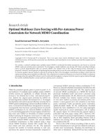
Figure 4 shows some profile curves of the distributions of
the clot components along the distance from the vessel wall.
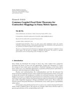
Figure 5 gives a comparison between the thrombi in
injuries of the wild-type and low FVII mice, which illustrates
how thrombi develop over time and the effects of FVII.
0
200
400

600
800
1000
1200
1 4 7 10131619222528313437404346495255586164
(+,+,+)
(+,+,−)
(+,−,+)
(+,−,−)
(−,+,+)
(−,+,−)
(−,−,+)
(−,−,−)
Volume (voxels)
Distance from the vessel wall
Figure 4: The profile curves of the distributions of the clot
components.
Here, laser-induced injuries were made in mesentery venules
(100 micron diameter). The results show that for a typical
clot of the wild ty pe, its volume increases rapidly at the
earlier time points and then shrinks significantly soon after
its peak; after a few minutes, the size of the clot becomes
relatively stable and does not change much. In contrast, while
platelets initially accumulate at the injury sites of low FVII
mice, the clot structures are unstable and embolize from
the vessel wall. Smaller thrombi do begin to form at later
times as some fibrin starts to accumulate in the thrombi.
The instability of the developing thrombi in the absence of
FVIIa-mediated fibrin generation can be seen from Figure 5.
The wild-type and low FVII thrombi also incorporate an

increasing number of blood cells (such as leukocytes and/or
erythrocytes).
Our analysis results show that, for a common wild-
type injury, the size of the clot usually peaks in one or
two minutes after the injury is made, and stabilizes about
two minutes after the peak. However, for low FVII injuries,
the size of the clot is not stable, with some significant
ups and downs in the size. We also observe more blood
cells covering the developing thrombi at later time points.
Further, as time goes, we see an increasing number of
6 EURASIP Journal on Advances in Signal Processing
Table 1: (A) is for a wild-typ e injury and (B) is for an FVII deficient type injury. The thrombi were at 1 minute after the injury.
(R,G,B) Vol. (A) % (A) Vol. (B) % (B)
(+, +, +) 36843 14.1695 783 6.4244
(+, +,
− ) 114525 44.0452 1084 8.894
(+,
− , +) 22596 8.6902 2853 23.4083
(+,
− , − ) 78190 30.0711 6875 56.4079
(
− ,+,+) 493 0.1896 8 0.0656
(
− ,+,− ) 3014 1.1592 185 1.5179
(
− , − ,+)0000
(
− , − , − ) 4356 1.6753 400 3.2819
Table 2: Porosity of a wild-type clot at different time points: T1 (40 seconds after injury), T 2 (80 seconds), and T6 (4 minutes).
Sample no. T1 Porosity (%) T2 Porosity (%) T6 Porosity (%)

1 59325 20.90 63333 15.56 69012 7.98
2 57746 23.00 63794 14.94 69581 7.23
3 58120 22.51 64041 14.61 68837 8.22
4 58901 21.47 64183 14.42 68540 8.61
5 58311 22.25 64370 14.17 69904 6.79
6 58019 22.64 64494 14.01 69331 7.56
7 57908 22.79 64450 14.07 68799 8.27
8 57899 22.80 64323 14.24 68736 8.35
9 58062 22.58 64139 14.48 69012 7.98
10 57803 22.93 63916 14.78 69538 7.28
fibrin/fibrinogen on the clot surface. That is, at the beginning
stage, there is a burst of platelets on the surface; however, the
number of fibrin/fibrinogen gradually increases and becomes
dominant. This is consistent with our hypothesis that the
fibril network on the clot surface is an important factor
which regulates thrombus growth and affects thrombus
stability. Figure 6 to some extent justifies our hypothesis.
It shows the composition of different components on the
surfaces of the clots; the curves indicate that, for wild-type
clots, the number of fibrin/fibrinogen gradually increases
over time. However, low FVII clots do not show this trend.
Here we use only two typical clots to illustrate our analysis.
Other wild-type/low FVII clots show a similar fashion of
growth.
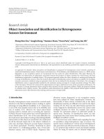
Figure 7 shows how the shape of a wild-type clot changes
in time (the clot structures are at 1, 1.5, and 4 minutes
after a laser-induced injury was made on the vessel wall).
We can clearly see in the figure that at later time points,
fibrin/fibrinogen cells (green voxels in the figure) become
dominant on the clot surface.

Other than the size and shape of a clot, another impor-
tant factor that may be related to the blood flow is the
permeability of the clot. A clot can be viewed as a porous
medium, and its permeability is measured by its porosity.
The porosity of a clot is represented by a percentage which
indicates the proportion of the void (i.e., nonclot) space in a
rectangular cuboid region which is entirely contained in the
volume of the clot. This percentage represents the ratio of
the total volume of the void space over the total volume of
the region of interest (the region normally includes both clot
and void voxels). To ensure the robustness of the percentage
value of porosity, after we select the initial position of the
“box” (i.e., cuboid region), we gradually move the box
around to check how consistent this ratio value is in nearby
locations. (In this experiment, we moved the box along
certain directions and used a step length of 2; for each box
size, we produced 10 sample values.) During the process of
moving the box, we maintain the same box size and make
sure that the entire box is always inside the clot volume.
Tab le 2 shows some experimental data. Here we use a box size
of 30
× 50 × 50. We counted the number of clot voxels inside
the box and calculated the porosity (we only calculated the
porosity of the wild-type clots, which grow in a more regular
fashion).
From Tab le 2, one can see that at the earlier time points,
a clot is more permeable than it is at the later time points.
As time goes, the clot tends to become more and more
compact. This is due largely to the fact that cells on and near
the clot surface (most of these cells are platelets at earlier

time points) are less a dhesive to each other than cells in the
inside and are easily flushed away by the blood flow. For
further analysis, two of the coauthors of this paper, Drs. Alber
and Xu, are leading a research effort aiming to construct a
multiscale simulation model for predicting how clots grow
under different flow conditions and different factors which
may regulate the clot growth [2].
EURASIP Journal on Advances in Signal Processing 7
0
20
40
60
80
100
120
140
160
180
×10
3
1 2 3 4 5 6 7 8 9 10 11 12 13 14 15
Volume (voxels)
Time (×40 seconds)
Wild-type mouse
(a)
0
2
4
6
8

10
12
1 2 3 4 5 6 7 8 9 10 11 12 13 14 15
Low FVII mouse
×10
3
Volume (voxels)
Time (×40 seconds)
Platelets
Fibrin
Platelets + fibrin
Cells
Total
(b)
Figure 5: The effects of FVII on the structures of venous thrombi.
6. Conclusions
We presented a new approach for segmentation, reconstruc-
tion, and analysis of 3D thrombi in 2-photon microscopic
images. Our method and platform have been applied to study
the structural differences between thrombi formed in wild-
type and low FVII mice. Thrombi in low FVII mice are
smaller, have a lower fibrin content, and are less stable than
those in wild-type mice.
Our platform for reconstruction and analysis of 3D
thrombi from 2-photon microscopic images will be a
valuable tool, allowing one to process a large amount of
images in a relatively short time. The high-resolution quanti-
tative structural analysis using our algorithms provides new
metrics that are likely to be critical to charac terizing and
understanding biomedically relevant features of thrombi.

For instance, the reconstructed str uctures of the develop-
ing thrombi (Figure 7) show the shapes of heterogeneous
subdomains of the clot enriched with different throm-
bus components. Since these subdomains have different
mechano-elastic properties, the interfaces between such
subdomains are potential sites responsible for structural
instability.
With the ability to provide a quantitative description
of the thrombus st ructures, it will be possible to com-
0
10
20
30
40
50
60
1 2 3 4 5 6 7 8 9 101112131415
Wild-type mouse
Time (×40 seconds)
×10
3
Volume (voxels)
(a)
0
1
2
3
4
5
6

7
8
9
123456789101112131415
Low FVII mouse
×10
3
Volume (voxels)
Time (×40 seconds)
Platelets
Fibrin
Platelets + fibrin
Cells
Total
(b)
Figure 6: The composition of different components on the clot
surface.
Figure 7: A reconstructed 3D clot as it changes in time (red for
platelets, green for fibrinogen/fibrin, and black for other blood
cells).
pare biological experimental thrombi monitored by mul-
tiphoton microscopy for their development in vivo with
the predictions of a multiscale computational model of
thrombogenesis [1, 2]. Such quantitative comparisons are
essential to the refinement and validation of the simulation
model. Currently, we have the individual modules and
procedures of the programs working, and the effectiveness
of our approaches has been shown by our experiments,
as discussed in Sections 4 and 5. However, the software
system as a whole is still under development (it is not

yet ready and available as a software tool to the research
community at this time, while we are working towards this
goal). Nevertheless, we anticipate that the integration of the
experimental and computational approaches for thrombo-
genesis made possible by our image processing strategies will
provide an effective tool for analyzing and understanding the
biomedically important yet complex processes of thrombus
development.
8 EURASIP Journal on Advances in Signal Processing
Acknowledgments
The authors would like to thank Amy Zollman for technical
assistance and Professor Kenneth W. Dunn and Profes-
sor Sherry G. Clendenon for assistance with multiphoton
microscopy. This research was supported in part by NSF
Grants CCF-0515203, CCF-0916606, and DMS-0800612,
NIH Grants R01-EB004640 and HL073750-01A1, and the
INGEN Initiative to Indiana University School of Medicine.
TheworkofX.Liuwassupportedinpartbyagraduate
fellowship from the Center for Applied Mathematics, Uni-
versity of Notre Dame.
References
[1] Z.Xu,N.Chen,M.M.Kamocka,E.D.Rosen,andM.Alber,
“A multiscale model of thrombus development,” Journal of the
Royal Society Interface, vol. 5, no. 24, pp. 705–722, 2008.
[2] Z. Xu, N. Chen, S. C. Shadden, et al., “Study of blood flow
impact on growth of thrombi using a multiscale model,” Soft
Matter, vol. 5, no. 4, pp. 769–779, 2009.
[3] X. Yang, H. Beyenal, G. Harkin, and Z. Lewandowski,
“Quantifying biofilm structure using image analysis,” Journal
of Microbiological Methods, vol. 39, no. 2, pp. 109–119, 1999.

[4] T. Zhu, H. C. Zhao, J. Wu, and M. F. Hoylaerts, “Three-
dimensional reconstruction of thrombus formation during
photochemically induced arterial and venous thrombosis,”
Annals of Biomedical Engineering, vol. 31, no. 5, pp. 515–525,
2003.
[5] N. Otsu, “A threshold selection method from gray-level his-
tograms,” IEEE Transactions on Systems, Man, and Cybernetics,
vol. 9, no. 1, pp. 62–66, 1979.
[6] M. I. Sezan, “A peak detection algorithm and its application to
histogram-based image data reduction,” Graphical Models and
Image Processing, vol. 29, pp. 47–59, 1985.
[7] G. Johannsen and J. Bille, “A threshold selection method using
information measures,” in Proceedings of the 6th International
Conference of Pattern Recognition (ICPR ’82), pp. 140–143,
Munich, Germany, 1982.
[8] S.K.Pal,R.A.King,andA.A.Hashim,“Automaticgreylevel
thresholding through index of fuzziness and entropy,” Pattern
Recognition Letters, vol. 1, no. 3, pp. 141–146, 1983.
[9] J.N.Kapur,P.K.Sahoo,andA.K.C.Wong,“Anewmethod
for gray-level picture thresholding using the entropy of the
histogram,” Computer Vision, Graphics, & Image Processing,
vol. 29, no. 3, pp. 273–285, 1985.
[10] R. L. Kirby and A. Rosenfeld, “A note on the use of (gray level,
local average gray level) space as an aid in threshold selection,”
IEEE Transactions on Systems, Man and Cybernetics, vol. 9, no.
12, pp. 860–864, 1979.
[11] B. Chanda and D. D. Majumder, “A note on the use of the
graylevel co-occurrence matrix in threshold selection,” Signal
Processing, vol. 15, no. 2, pp. 149–167, 1988.
[12] D. Z. Chen, M. Smid, and B. Xu, “Geometric algorithms

for density-based data clustering,” International Journal of
Computational Geometry and Applications,vol.15,no.3,pp.
239–260, 2005.
[13] M. Ester, H P. Kriegel, J. Sander, and X. Xu, “A density-based
algorithm for discovering clusters in large spatial databases
with noise,” in Proceedings of 2nd International Conference on
Knowledge Discovery and Data Mining (KDD ’96), pp. 226–
231, Portland, Ore, USA, 1996.
[14] M. E. Celebi, Y. A. Aslandogan, and P. R. Bergstresser,
“Mining biomedical images with density-based clustering,”
in Proceedings of International Conference on Information
Technology: Coding and Computing (ITCC ’05), vol. 1, pp. 163–
168, Las Vegas, Nev, USA, April 2005.
[15] Y. Song, C. Xie, Y. Zhu, C. Li, and J. Chen, “Function based
medical image clustering analysis and research,” Advances in
Computer, Information, and Syste m s Sciences, and Engineering,
pp. 149–155, 2006.
[16] P K. Chan, S H. Cheng, and T C. Poon, “Automated
segmentation in confocal images using a density clustering
method,” Journal of Electronic Imaging, vol. 16, no. 4, Article
ID 043003, 9 pages, 2007.
[17] B. Herman, M. J. Parry-Hill, I. D. Johnson, and M. W.
Davidson, “Introduction to optical microscopy,” 2003,
/>photobleaching/index.html.
[18] B. Weiss, “Fast median and bilateral filtering,” ACM Transac-
tions on Graphics, vol. 25, no. 3, pp. 519–526, 2006.
[19] M. Ester, H P. Kriegel, J. Sander, and X. Xu, “A density-based
algorithm for discovering clusters in large spatial databases
with noise,” in Proceedings of the 2nd International Conference
on Knowledge Discovery and Data Mining (KDD ’96), pp. 226–

231, Portland, Ore, USA, 1996.
[20] E. R. Dougherty, An Introduction to Morphological Image
Processing, SPIE Optical Engineering Press, Center for Imaging
Science Rochester Institute of Technology, Bellingham, Wash,
USA, 1992.
[21] W. E. Lorensen and H. E. Cline, “Marching cubes: a high
resolution 3D surface construction algorithm,” Co mputer
Graphics, vol. 21, no. 4, pp. 163–169, 1987.
[22] H. Edelsbrunner and E. P. Mucke, “Three-dimensional alpha
shapes,” ACM Transactions on Graphics, vol. 13, no. 1, pp. 43–
72, 1994.