Parallel Manipulators New Developments Part 2 pot

2
Application of Neural Networks to Modeling and
Control of Parallel Manipulators
Ahmet Akbas
Marmara University
Turkey
1. Introduction
There are mainly two types of the manipulators: serial manipulators and parallel
manipulators. The serial manipulators are open-ended structures consisting of several links
connected in series. Such a manipulator can be operated effectively in the whole volume of
its working space. However, as the actuator in the base has to carry and move the whole
manipulator with its links and actuators, it is very difficult to realize very fast and highly
accurate motions by using such manipulators. As a consequence, there arise the problems of
bad stiffness and reduced accuracy.
Unlike serial manipulators their counterparts, parallel manipulators, are composed of
multiple closed-loop chains driving the end-effector collectively in a parallel structure. They
can take a large variety of form. However, most common form of the parallel manipulators
is known as platform manipulators having architecture similar to that of flight simulators in
which two special links can be distinguished, namely, the base and moving platform. They
have better positioning accuracy, higher stiffness and higher load capacity, since the overall
load on the system is distributed among the actuators.
The most important advantage of parallel manipulators is certainly the possibility of
keeping all their actuators fixed to base. Consequently, the moving mass can be much
higher and this type of manipulators can perform fast movements. However, contrary to
this situation, their working spaces are considerably small, limiting the full exploitation of
these predominant features (Angeles, 2007).
Furthermore, for the fast and accurate movements of parallel manipulators it is required a
perfect control of the actuators. To minimize the tracking errors, dynamical forces need to be
compensated by the controller. In order to perform a precise compensation, the parameters
of the manipulator’s dynamic model must be known precisely.
However, the closed mechanical chains make the dynamics of parallel manipulators highly

complex and the dynamic models of them highly non-linear. So that, while some of the
parameters, such as masses, can be determined, the others, particularly the firiction
coefficients, can’t be determined exactly. Because of that, many of the control methods are
not efficient satisfactorly. In addition, it is more difficult to investigate the stability of the
control methods for such type manipulators (Fang et al., 2000).
Under these conditions of uncertainty, a way to identify the dynamic model parameters of
parallel manipulators is to use a non-linear adaptive control algorithm. Such an algorithm
Parallel Manipulators New Developments

22
can be performed in a real-time control application so that varying parameters can
continuously be updated during the control process (Honegger et al., 2000).
Another way to identify the dynamic system parameters may be using the artificial
intelligence (AI) techniques. This approach combines the techniques from the fields of AI
with those of control engineering. In this context, both the dynamic system models and their
controller models can be created using artificial neural networks (ANN).
This chapter is mainly concerned with the possible applications of ANNs that are contained
within the AI techniques to modeling and control of parallel manipulators. In this context, a
practical implementation, using the dynamic model of a conventional platform type parallel
manipulator, namely Stewart manipulator, is completed in MATLAB simulation
environment (www.mathworks.com).
2. ANN based modeling and control
Intelligent control systems (ICS) combine the techniques from the fields of AI with those of
control engineering to design autonomous systems. Such systems can sense, reason, plan,
learn and act in an intelligent manner, so that, they should be able to achieve sustained
desired behavior under conditions of uncertainty in plant models, unpredictable
environmental changes, incomplete, inconsistent or unreliable sensor information and
actuator malfunction.
An ICS comprises of perception, cognition and actuation subsystems. The perception
subsystem collects information from the plant and the environment, and processes it into a

form suitable for the cognition subsystem. The cognition subsystem is concerned with the
decision making process under conditions of uncertainty. The actuation subsystem drives
the plant to some desired states.
The key activities of cognition systems include reasoning, using knowledge-based systems
and fuzzy logic; strategic planning, using optimum policy evaluation, adaptive search,
genetic algorithms and path planning; learning, using supervised or unsupervised learning
in ANNs, or adaptive learning (Burns, 2001).
In this chapter it is mainly concerned with the application of ANNs that are contained
within the cognition subsystems to modeling and control of parallel manipulators.
2.1 ANN overwiev
ANN is a network of single neurons jointed together by synaptic connections. Such that they
are organized as neuronal layers. Each neuron in a particular layer is connected to neurons
in the subsequent layer with a weighted synaptic connection. They attempt to emulate their
biological counterparts.
2.1.1 Perceptrons
McCulloch and Pitts was started first study on ANN in 1943. They proposed a simple model
of neuron. In 1949 Hebb described a technique which became known as Hebbian learning.
In 1961 Rosenblatt devised a single layer of neurons, called a perceptron that was used for
optical pattern recognition (Burns, 2001)
Perceptrons are early ANN models, consisting of a single layer and simple threshold
functions. The architecture of a perceptron consisting of multiple neurons with Nx1 inputs
and Mx1 outputs is shown in Fig. 1. As seen in this figure, the output vector of the
Application of Neural Networks to Modeling and Control of Parallel Manipulators

23
perceptron is calculated by summing the weighted inputs coming from its input links, so
that
u = W p + b (1)
q = f(u) (2)
where p is Nx1 input vector (p

1
, p
2
, p
N
)
,
W is MxN weighting coefficients matrix (w
11
, w
12
,
w
1N ; ;
w
j1
, w
j2
, , w
jN
; ; w
M1
, w
M1
, ,w
MN
), b is Mx1 bias factor vector, u is Nx1 vector
including the sum of the weighted inputs (u
1
, u

2
, u
M
) and bias vector, q is Mx1 output
vector (q
1
, q
2
, q
M
)
,,
and f(.) is the activation function.

N
N x 1
inputs
p
W
b1
M x N
M x 1
u
M x 1
M
q
M x 1
hard limit layer outputs

Fig. 1. The architecture of a perceptron

In early perceptron models, the activation function was selected as hard-limiter (unit step)
given as follows:

0)(
0<)(
,1
,0
=
¡Ý
i
i
i
uf
uf
q
(3)
where i = 1,2,…,M denotes the number of neuron in the layer, u
i
weighted sum of its
particular neuron, and q
i
its output. However, in any ANN the activation function f (u
i
) can
take many forms, such as, linear (ramp), hyperbolic tangent and sigmoid forms. The
equation for sigmoid function is:
f (u
i
) = 1 / (1 + e
-u

i
) (4)
The sigmoid activation function given in Equation (4) is popular for ANN applications since
it is differantiable and monolithic, both of which are a requirement for training algorithms
like as the backpropagation algorithm.
Perceptrons must include a training rule for adjusting the weighting coefficients. In the
training process, it compares the actual network outputs to the desired network outputs for
each epoch to determine the actual weighting coefficients:
e = q
d
– q (5)
W
new
= W
old
+ e p
T
(6)
Parallel Manipulators New Developments

24
b
new
= b
old
+ e (7)
where e is Mx1 error vector, q
d
is Mx1 target (desired) vector, the upscripts T , old and new
denotes the transpose, the actual and previous (old) representation of the vector or matrix,

respectively (Hagan et al., 1996).

2.1.2 Network architectures
There are mainly two types of ANN architectures: feedforward and recurrent (feedback)
architectures. In the feedforward architecture, all neurons in a particular layer are fully
connected to all neurons in the subsequent layer. This generally called a fully connected
multilayer network. Recurrent networks are based on the work of Hopfield and contain
feedback paths. A recurrent network having two inputs and three outputs is shown in Fig. 2.
In Fig. 2, the inputs occur at time (kT) and the outputs are predicted at time (k+1)T, where k
is discrete time index and T is sampling time, respectively.

∑
∑
∑
f
f
f
u
1
u
2
u
3
q
3
(k+1)T
b
1
1
b

2
1
b
3
1
q
2
(k+1)T
q
1
(k+1)T
z
-1
z
-1
z
-1
q
3
(kT)
q
2
(kT)
q
1
(kT)
p
1
(kT)
p

2
(kT)

Fig. 2. Recurrent neural network architecture
Then the network can be represented in matrix form as:
q(k+1)T = f (W
1
p(kT) + W
2
q(kT) + b) (8)
where b is bias vector, f(.) is activation function, W
1
and W
2
are weight matrix for inputs and
feedback paths, respectively.
2.1.3 Learning
Learning in the context of ANNs is the process of adjusting the weights and biases in such a
manner that for given inputs, the correct responses, or outputs are achieved. Learning
algorithms include supervised learning and unsupervised learning.
In the supervised learning the network is presented with training data that represents the
range of input possibilities, together with associated desired outputs. The weights are
adjusted until the error between the actual and desired outputs meets some given minimum
value.
Application of Neural Networks to Modeling and Control of Parallel Manipulators

25
Unsupervised learning is an open-loop adaption because the technique does not use
feedback information to update the network’s parameters. Applications for unsupervised
learning include speech recognition and image compression.

Important unsupervised learning include the Kohonen self-organizing map (KSOM), which
is a competitive network, and the Grossberg adaptive resonance theory (ART), which can be
for on-line learning.
There are multitudes of different types of ANN models for control applications. The first
one of them was by Widrow and Smith (1964). They developed an Adaptive LINear Element
(ADLINE) that was taught to stabilize and control an inverted pendulum. Kohonen (1988)
and Anderson (1972) investigated similar areas, looking into associative and interactive
memory, and also competitive learning (Burns, 2001).
Some of the more popular of ANN models include the multi-layer perceptron (MLP) trained
by supervised algorithms in which backpropagation algorihm is used.
2.1.4 Backpropagation
The backpropagation algorithm was investigated by Werbos (1974) and futher developed by
Rumelhart (1986) and others, leading to the concept of the MLP. It is a training method for
multilayer feedforward networks. Such a network including N inputs, three layers of
perceptrons, each has L1, L2, and M neurons, respectively, with bias adjustment is shown in
Fig. 3.

inputs
∑
∑
∑
f
1
f
1
f
1
u
1
1

u
1
2
u
1
L1
p
1
p
2
p
3
p
N
∑
∑
∑
f
2
u
2
1
u
2
2
u
2
L2
∑
∑

∑
u
3
1
u
3
2
u
3
M
f
2
f
2
f
3
f
3
f
3
q
3
1
q
3
2
q
3
M
q

2
1
q
2
2
q
2
L2
q
1
1
q
1
2
q
1
L1
w
2
1,1
w
2
L2, L1
w
1
1,1
w
3
M,L2
w

1
1,1
w
1
L1, N
first layer second layer third layer
q
1
= f
1
(W
1
p + b
1
) q
2
= f
2
(W
2
q
1
+ b
2
) q
3
= f
3
(W
3

q
2
+ b
3
)q
0
=

p
q
3
= f
3
(W
3
f
2
(W
2
f
1
(W
1
p + b
1
)+ b
2
)+ b
3
)

b
1
1
1
b
1
2
1
b
1
L1
1
b
2
1
1
b
2
2
1
b
2
L2
1
b
3
M
1
b
3

2
1
b
3
1
1

Fig. 3. Three-layer feedforward network
First step in backpropogation is propagating the inputs towards the forward layers through
the network. For L layer feedforward network, training process is stated from the output
layer:
q
0
= p
q
l+1
= f
l+1
(W
l+1
q
l
+ b
l+1
) , l = 0 , 1, 2,…., L-1 (9)
q = q
L
Parallel Manipulators New Developments

26

where l is particular layer number; f
l
and W
l
represent the activation function and weighting
coefficients matrix related to the layer l, respectively.
Second step is propagating the sensivities (s) from the last layer to the first layer through the
network: s
L
, s
L-1
, s
L-2
,…, s
l
…, s
2
, s
1
. The error calculated for output neurons is propagated to
the backward through the weighting factors of the network. It can be expressed in matrix
form as follows:


)-( ( qquFs
dLLL
) 2
•
−=
,

11
( )(
++
•
=
lllll
sWuFs
T
)
, for l = L-1,…, 2, 1 (10)
where
)(
ll
uF
•
is Jacobian matrix which is described as follows

⎥
⎥
⎥
⎥
⎥
⎥
⎥
⎥
⎥
⎦
⎤
⎢
⎢

⎢
⎢
⎢
⎢
⎢
⎢
⎢
⎣
⎡
∂
∂
∂
∂
∂
∂
=
•
l
N
l
N
l
l
2
l
2
l
l
1
l

1
l
l
u
uf
u
uf
u
uf
)(
00
0
)(
0
00
)(
)(u
l
"
###
"
"
F

(11)

Here N denotes the number of neurons in the layer l. The last step in backpropagation is
updating the weighting coefficients. The state of the network always changes in such a way
that the output follows the error curve of the network towards down:
W

l
(k+1) = W
l
(k) - α s
l
(q
l-1
)
T
(12)
b
l
(k+1) = b
l
(k) - α s
l
(13)
where α represents the training rate, k represents the epoch number (k=1,2,…,K).

By the
algorithmic approach known as gradient descent algorithm using approximate steepest
descent rule, the error is decreased repeatedly (Hagan, 1996).
2.2 Applications to parallel manipulators
ANNs can be used for modeling various non-linear system dynamics by learning because of
their non-linear system modelling capability. They offer highly parallel, adaptive models
that can be trained by using system input-output data.

ANNs have the potential advantages for modeling and control of dynamic systems, such
that, they learn from experience rather than by programming, they have the ability to
generalize from given training data to unseen data, they are fast, and they can be

implemented in real-time.
Possible applications using ANN to modeling and control of parallel manipulators may
include:
• Modeling the manipulator dynamics,
• Inverse model of the manipulator,
• Controller emulation by modeling an existing controller,
• Various intelligent control applications using ANN models of the manipulator and/or
its controller. Such as, ANN based internal model control (Burns, 2001).
Application of Neural Networks to Modeling and Control of Parallel Manipulators

27
2.2.1 Modeling the manipulator dynamics
Providing input/output data is available, an ANN may be used to model the dynamics of
an unknown parallel manipulator, providing that the training data covers whole envelope
of the manipulator operation (Fig. 4).
However, it is difficult to imagine a useful non-repetitive task that involves making random
motions spanning the entire control space of the manipulator system. This results an
intelligent manipulator concept, which is trained to carry out certain class of operations
rather than all virtually possible applications. Because of that, to design an ANN model of
the chosen parallel manipulator training process may be implemented on some areas of the
working volume, depending on the structure of chosen manipulator (Akbas, 2005). For this
aim, the manipulator(s) may be controlled by implementation of conventional control
algorithms for different trajectories.



Fig. 4. Modelling the forward dynamics of a parallel manipulator
If the ANN in Fig. 4 is trained using backpropagation, the algorithm will minimize the
following performance index:

() ()( )() ()()
(
)
∑
=
−−=
N
n
t
kTqkTqkTqkTqPI
1
ˆˆ
(14)
where q and

^
q
denote the output vector of the manipulator and ANN model, respectively.
2.2.2 Inverse model of the manipulator
The inverse model of a manipulator provides a control vector τ(kT), for a given output
vector q(kT) as shown in Fig. 5. So, for a given parallel manipulator model, the inverse
model could be trained with the parameters reflecting the forward dynamic characteristics
of the manipulator, with time.

Parallel Manipulators New Developments

28

Fig. 5. Modelling the inverse dynamics of parallel manipulator

As indicated above, the training process may be implemented using input-output data
obtained by manipulating certain class of operations on some areas of the working volume
depending on the structure of chosen manipulator.
2.2.3 Controller emulation
A simple application in control is the use of ANNs to emulate the operation of existing
controllers (Fig. 6).


Fig. 6. Training the ANN controller and its implementation to the control system
It may be require several tuned PID controllers to operate over the constrained range of
control actions. In this context, some manipulators may be required more than one emulated
controllers that can be used in parallel form to improve the reliability of the control system
by error minimization approach.
2.2.4 IMC implementation
ANN control can be implemented in various intelligent control applications using ANN
models of the manipulator and/or its controller. In this context the internal model control
Application of Neural Networks to Modeling and Control of Parallel Manipulators

29
(IMC) can be implemented using ANN model of parallel manipulataor and its inverse
model (Fig. 7).



Fig. 7. IMC application using ANN models of parallel manipulator
In this implementation an ANN model model replaces the manipulator model, and an
inverse ANN model of the manipulator replaces the controller as shown in Fig. 7.
2.2.5 Adaptive ANN control
All closed-loop control systems operate by measuring the error between desired inputs and
actual outputs. This does not, in itself, generate control action errors that may be

backpropagated to train an ANN controller. However, if an ANN of the manipulator exists,
backpropagation through this network of the system error will provide the necessary
control action errors to train the ANN controller as shown in Fig.8.




Fig. 8. Control action generated by adaptive ANN controller
3. The structure of Stewart manipulator
Six degrees of freedom (6-dof) simple and practical platform type parallel manipulator,
namely Stewart manipulator, is sketched in Fig. 9. These type manipulators were first
introduced by Gough (1956-1957) for testing tires. Stewart (1965) suggested their use as
flight simulators (Angeles, 2007).
Parallel Manipulators New Developments

30
0
13
1
2
3
4
5
6
7
8
9
10
11
12

Moving Platform
B
Base Platform
P

Fig. 9. A sketch of the 6-dof Stewart manipulator
In Fig. 9, the upper rigid body forming the moving platform, P, is connected to the lower
rigid body forming the fixed base platform, B, by means of six legs. Each leg in that figure
has been represented with a spherical joint at each end. Each leg has upper and lower rigid
bodies connected with a prismatic joint, which is, in fact, the only active joint of the leg. So,
the manipulator has thirteen rigid bodies all together, as denoted by 1,2… 13 in Fig. 9.
3.1 Kinematics
Motion of the moving platform is generated by actuating the prismatic joints which vary the
lengths of the legs, q
L
i
, i = 1….6. So, trajectory of the center point of moving platform is
adjusted by using these variables.
For modeling the Stewart manipulator, a base reference frame F
B
(O
B
x
B
y
B
z
B
) is defined as
shown in Fig. 10. A second frame F

P
(O
P
x
P
y
P
z
P
) is attached to the center of the moving
platform, O
P
, and the points linking the legs to the moving platform are noted as Q
i
, i =
1….6, and each leg is attached to the base platform at the point B
i
, i = 1….6.
The pose of the center point, O
P
, of moving platform is represented by the vector
x = [x
B
y
B
z
B
α β γ]
T
(15)

where x
B
, y
B
, z
B
are the cartesian positions of the point O
P
relative to the frame F
B
and α, β, γ
are the rotation angles, namely Euler angles, representing the orientation of frame F
P

relative to the frame F
B
by three successive rotations about the x
P
, y
P
and z
P
axes, given by
the matrices R
x
(α), R
y
(β), R
z
(γ) respectively (Spong & Vidyasagar, 1989). Thus, the rotation

matrix between the F
B
and F
P
frames is given as follows:

)( )( )( = γRβRαRR
zyx
P
B
(16)
Application of Neural Networks to Modeling and Control of Parallel Manipulators

31

Fig. 10. Assignments for kinematic analysis of the Stewart manipulator
Then we can analyze the inverse kinematics of Stewart manipulator by the representation of
any one of its legs. For a given pose of the center point of moving platform, O
P
, the defining
vectors are shown in Fig. 11.


Fig. 11. Defining the vectors for a given pose of the moving platform
Parallel Manipulators New Developments

32
By using the rotation matrix given by equation (16), the position vector of the upper joint
position, Q
i

, connecting the moving platform to the leg i, q
Q
i
can be transformed to the
frame F
B
as follows:

i
P
B
OQ
i
R dpq + =
i = 1….6 (17)
where p
O
represents the position vector of the center point of moving platform, O
P
, relative
to the frame F
B
, d
i
is the position vector of the point Q
i
, i = 1….6, relative to the frame F
P
.
Then the vector q

A
i
representing the leg legths between the joint points B
i
and Q
i
can be
transformed to the frame F
B
as follows:

Q
ii
A
iii
QB qa q +-==
→
i = 1….6 (18)
where a
i
represents the position vector of the point B
i
, i = 1….6, relative to the frame F
B
.
The leg lengths q
A
i
, i = 1….6, is then obtained by Euclidean norm of the leg vector given
above. So, using equation (17) and (18) we can write (Zanganeh et al., 1997)

) () ( )
2
i
P
B
O
i
T
i
P
B
O
i
A
i
RRq dpadpa ++= ++(
, i = 1….6 (19)
The leg lengths related to a given pose of moving platform can be obtained for a trajectory
defined by the pose vector, x, given in equation (15). Considering a circular motion depicted
as in Fig. 12, the trajectory of moving platform with zero rotation angles ([α β γ] = [0 0 0]) is
given as follows:

Fig. 12. A circular motion trajectory of the moving platform
x = [(p
O
)
T
0 0 0]
T

= A(t) x
0
(20)
where p
O
= [x
B
y
B
z
B
]
T
denotes the 3x1 position vector of the center point of moving
platform, A(t) is a 6x6 matrix and x
0
is a 6x1 coeeficient vector given as below
Application of Neural Networks to Modeling and Control of Parallel Manipulators

33
()
(
)
[
]
()
[]
(
)
[]

()
[]
⎥
⎥
⎥
⎥
⎦
⎤
⎢
⎢
⎢
⎢
⎣
⎡
−
=
00
0
1
0
0
0
cos
sin
0
sin
cos
t
t
t

t
tA
θ
θ
θ
θ

(21)
x
0
= [0

r

h

0 0 0]
T
(22)
where O denotes the 3x3 zero matrix, h is the hight of the center point of moving platform
with respect to base frame, and r is the radius of the circle.
The Jacobian matrix that gives the relation between the prismatic joint velocities and the
velocity of the center point of moving platform, O
P
, can be derived using the partial
differentiation of the inverse geometric model of the manipulator given in equation (19).
3.2 Dynamics
As descripted in Fig. 9, Stewart manipulator has thirteen rigid bodies. The Newton-Euler
equations of the manipulator can be derived in a more compact form as described below
(Fang et al., 2000; Khan et al., 2005):

Let the 6x6 matrix M
i
, denoting the mass and moment of inertia properties of the rigid body
i be

⎥
⎦
⎤
⎢
⎣
⎡
×
=
10
0
i
i
i
m
I
M

, i = 1….13 (23)

where O and 1 denote the 3x3 zero and identity matrices; I
i
is inertia matrix defined with
respect to the mass center, C
i
, of the body i ; m

i
is the mass of the body i. Let c
i
and ċ
i
denote
the position and velocity vectors of C
i
, and ω
i
denote the angular velocity vector of C
i
. Then
the wrench vector t
i
is defined in terms of the angular and linear velocities as follows:


⎥
⎥
⎦
⎤
⎢
⎢
⎣
⎡
⋅=
i
i
i

c
t
ω

, i = 1….13 (24)
Let the 6x6 matrix Ω
I
, denoting the angular velocity of the rigid body i be


⎥
⎦
⎤
⎢
⎣
⎡
=Ω
00
0
i
i
ω

, i = 1….13 (25)
where, O denotes the 3x3 zero matrix. The generalized matrices given in equation (23) and
(25) are block symmetrical, as follows:

(
)
(

)
13211321
, ,,,, ,,
Ω
Ω
Ω
=
Ω
=
diagMMMdiagM
(26)
Then, the generalized wrench matrix t can be expressed as follows
t=[t
1
T
t
2
T
t
13
T
]
T
(27)
For the system having constraint on velocity, the constraint of velocity can be expressed by
following equation:
Dt=0 (28)
Let T be the natural orthogonal complement (NOC) of the coefficient matrix D related to the
constraint equation (28) of velocity. Hence, employing the joint coordinates
6

R∈q
as
Parallel Manipulators New Developments

34
generalized coordinate vector, we can get the dynamic model of system, which don’t
contain the constraint forces.

τqGqqq,CqqM =)( + )( + (
••••
)

(29)
where M(q) is a symmetrical and positive definition matrix as given below;

6x6
R =)( ∈ TMTqM
T
(30)
C is the coefficient matrix of the vectors of Coriolis and centripetal force as given below;

MTT TMTqq,C C Ω + = )(=
••
TT
(31)
q is the generalized coordinate vector,
6
R∈τ
is the generalized force (driving force) vector,
respectively. G(q) is the gravity vector as given below;

gg
WTqτqG
T
= )( = )(
(32)
where W
g
are wrenches vector due to gravity:

TTT
TTT
mm ] , ,. ,[=] , ,[ =
T
g0g0 WWWW
131
g
13
g
2
g
1
g
(33)
where 0 is 3x1 zero vector, g is the vector of acceleration of gravity.
4. Controller emulation by using Elman networks
In this stage, it is aimed to implement an application of ANN to emulate the operation of an
existing PID controller in a Stewart manipulator control system. This system is given as a
control system example for MATLAB applications (www.mathworks.com). The block
diagram of the control system is given in Fig. 13.

Fig. 13. Srewart manipulator control system using PID controller
As shown in this figure, trajectory generator calculates the leg lengths, which are desired leg
lengths formed as a 6x1 q
D
vector feeding the PID controller input, by using the inverse
kinematic model of Stewart manipulator. PID controller produces a 6x1 control vector, τ,
consisting of the leg forces applied to the prismatic joint actuators of the manipulator. In
response, the dynamic model of the manipulator produces two 6x1 output vectors, q
A
and
ċ=
.
q
A
, which include actual leg lengths and actual linear leg velocities, respectively. These
are fed back to the controller. So, the controller has 18 inputs and 6 outputs totally. PID
Application of Neural Networks to Modeling and Control of Parallel Manipulators

35
controller compares the actual and desired leg lengths to generate the error vector feeding
its proportional and integral inputs. In the same time, the velocity feedback vector feeds the
derivative input of the controller.
Designing an ANN emulation of controller generalized for the whole area of working space
is more difficult task. It is also difficult to imagine a useful non-repetitive task that involves
making random motions spanning the entire control space of the manipulator system. This
results an intelligent manipulator concept, which is trained to carry out certain class of
operations rather than all virtually possible applications (Akbas, 2005).
On the other hand, since the parallel manipulators have more complex dynamic structures,

training process may be required much more data then other type plants. So, it can be
taught to design more than one ANN controller trained by different input-output data sets,
and use them in a parallelly formed controller structure instead of unique ANN controller
structure. This can improve the reliability of the controller. Because of that, three ANN
controllers are trained and they are used in parallel form in this case study.
4.1 Training
Due to its profound impact on the learning capability and networking performance, Elman
network having recurrent structure is selected for training. Three of them, each have 18
inputs and 6 outputs, are trained by using PID controller input-output data. For this aim,
input-output data are prepared during the implementation of the PID controller to the
Stewart manipulator.
During the data log phase, manipulator is operated in a constrained area of its working
space. For this aim, the manipulator is controlled by implementation of different trajectories
selected uniformly in a planar sub-space, created as given example in equations (21) and
(22) also as given in Fig. 12. Load variations are taken into consideration to generate the
training data.
Three sets of input-output data each have 5000 vectors are generated by MATLAB
simulations for each of Elman networks. MATLAB ANN toolbox is used for off-line training
of Elman networks. Conventional backpropagation algorithm, which uses a threshold with a
sigmoidal activation function and gradient descent error-learning, is used. Learning and
momentum rates are selected optimally by MATLAB program. The numbers of neurons in
the hidden layers are selected experimentally during the training. These are used as 40, 30
and 50, respectively for each network.
4.2 Implementation
After the off-line training, three of Elman networks are prepared as embedded Simulink
blocks with obtained synaptic weights. To improve the reliability of the controller by error
minimization approach, they are used in a parallel structure and embedded to the control
system block diagram (Fig. 14). In this figure, parallely-implemented Elman ANN controller
is represented in a block form. Its detailed representation is given in Fig. 15.
In this implementation, the force values generated by three Elman networks are applied to

the inputs of the corresponding manipulator’s dynamic model. Error vector is computed for
each of the ANN by using the difference between the actual leg lengths generated by
manipulator’s dynamic model and the desired leg lengths. The results are evaluated to
select the network generating the best result. Then it is assigned as the ANN controller for
actual time step, and its output is assigned as the force output of the parallely-implemented
Elman ANN controller output driving the manipulator’s dynamic model (instead of a real
manipulator, in this case).
Parallel Manipulators New Developments

36
Trajectory
Generator
Elman ANN
Cntrl
Stewart
Mnpl.
Dynamic
Model
τ
q
D
(k-1)
q
A
(k)
c(k)
.
= q
A
(k)

.
(k)
q
A
(k)
q
A
(k)
.
x (t) x
A
(k)
Stewart
Mnpl
Kinematic
Model
Fig. 14. ANN controller implementation to the manipulator control system
4.3 Simulation results
To compare the performance of the created ANN controller, the Srewart manipulator
control system is operated both by the PID controller, and the parallelly-implemented
Elman ANN controller for T=4 s. simulations. For these operations, a trajectory like as given
with equations (21) and (22) is created with the parameter assignments: h = 2 m, r = 0.02 m.
Also θ(t) parameter is used as follows:

T ¡Ü ¡Ü0 ,
T
2
= tt
π
θ(t)

(34)
During the simulations, the sampling period is chosen, as 0.001 s. So, totally 4000 steps are
included in each simulation.

Elman
ANN
Cntrl-1
i = 1
Evaluation
and
Selection
of the best
performance
ANN
output
Trajectory
Generator
x (t)
Elman
ANN
Cntrl-1
i = 2
Elman
ANN
Cntrl-1
i = 3
1
τ
(k)
2

τ
3
τ
Stewart
Mnpl
Dyn.
Model
Stewart
Mnpl
Dyn.
Model
Stewart
Mnpl
Dyn.
Model
(k)
(k)
q
A
1
(k)
q
A
1
(k)
.
q
D
(k-1)
q

A
2
(k)
q
A
2
(k)
.
q
A
3
(k)
q
A
3
(k)
.
q
D
(k-1)
τ
(k) =
i
τ
(k)
Parallely-implemented Elman ANN Controller
1
τ
(k)
2

τ
(k)
3
τ
(k)

Fig. 15. The structure of parallelly-implemented Elman ANN controller
Application of Neural Networks to Modeling and Control of Parallel Manipulators

37
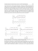
An example of the variations of the force outputs generated by both controllers is shown in
Fig. 16, for the first leg of the manipulator. Fig. 16a and Fig. 16b show the force output of the
PID controller and parallely-implemented Elman ANN controller, respectively. In these
simulations, it has been observed that, the error between the two controller outputs is a little
more at the starting phase of the simulations then the remaining times.
However, it can be said that, ANN controller emulates the PID controller successfully as a
whole for the given trajectory.

(a)

(b)
Fig.16. Force outputs of the controllers applied to the first leg of the Stewart manipulator
(a)-PID controller output, (b)-ANN controller output
Similar adaptations are obtained for the control system output. For the given trajectory,
position errors obtained by averaging the sum of the square errors relative to the desired
position of the center point of moving platform both for the PID controller and ANN
controller is given in Table 1. As seen in this table obtained position error values due to the
x
B
, y

B
and z
B
variations have too small changes.


Table 1. The sum of the squares of the position errors obtained by PID and ANN
Parallel Manipulators New Developments

38
During simulations, variations of the x
B
, y
B
and z
B
positions of the center point of moving
platform are given in Fig. 17, so that, Fig. 17a and Fig. 17b show the variation of actual x
B
, y
B

and z
B
positions obtained simulations using PID controller and parallely-implemented
Elman ANN controller, respectively. As seen, the tracing error between the two control
modes is a little more at the starting phase only. This is due to instantaneous big difference
between the desired y
B
position and its starting value. However, tracing the desired

positions by PID controller is well emulated by parallely-implemented Elman ANN
controller, as a whole.



(a)
Application of Neural Networks to Modeling and Control of Parallel Manipulators

39



(b)
Fig.16. Variation of actual position of the center point of moving platform, in simulations
(a)-Obtained by the PID controller, (b)- Obtained by the ANN controller
5. Conclusion
This chapter is mainly concerned with the application of ANNs to modeling and control of
parallel manipulators. A practical implementation is completed to emulate the operation of
Parallel Manipulators New Developments

40
an existing PID controller in a Stewart manipulator control system. It can be said that,
excepted results has been achieved for this case study.
Since the parallel manipulators have more complex dynamic structures, depending on the
chosen type of applications training process it may be required much more data then in this
case. So, designing an ANN for applications including the whole area of working space is
more difficult task. It is also difficult to imagine a useful non-repetitive task that involves
making random motions spanning the entire control space of the manipulator system.
However, for a succesfull study, it may have an important role selecting the type and
structure of ANN by experience, depending on the requirements of the chosen application.

6. References
Akbas, A. (2005). Intelligent predictive control of a 6-dof robotic manipulator with reliability
based performance improvement, Proceedings of the 6th International Conference on
Intelligent Data Engineering and Automated Learning, LNCS Vol. 3578, pp. 272-279,
ISBN: 3-540-26972-X, Brisbane, Australia, July 2005, Springer
Angeles, J. (2007). Fundamentals of Robotic Mechanical Systems, Theory, Methods, and
Algorithms, Springer Science+Business Media, LLC, ISBN: 0 387 29412 0, NY, USA
Burns, R.S. (2001). Advanced Control Engineering, Butterworth-Heinemann, ISBN: 0 7506 5100
8, Oxford
Fang, H.; Zhou, B.; Xu, H. & Feng, Z. (2000). Stability analysis of trajectory tracing contro1 of
6-dof parallel manipulator, Proceedings of the 3d World Congress on Intelligent Control
and Automation, IEEE, Vol. 2, pp. 1235-1239, ISBN: 0-7803-5995-X, Hefei, China, June
28-July 2, 2000
Hagan, M.T.; Demuth, H.B. & Beale, M. (1996). Neural Network Design, PWS Publishing
Company- Thompson Learning, ISBN: 7 111 10841 8, USA
Honegger, M.; Brega, R. & Schweitzer, G. (2000). Application of a nonlinear adaptive
controller to a 6 dof parallel manipulator, Proceedings of the 2000 IEEE International
Conference on Robotics and Automation, ICRA 2000, pp. 1930-1935, ISBN: 0-7803-5889-
9, San Francisco, CA, USA, April 24-28, 2000
Khan, W.A.; Krovi, V.N.; Saha, S.K. & Angeles, J. (2005). Modular and recursive kinematics
and dynamics for parallel manipulators. Multibody System Dynamics, Vol. 14, No.3-
4, Nov. 2005, pp. 419-455, ISSN: 1384-5640, Springer
Spong, M.W. & Vidyasagar, M. (1989). Robot Dynamics and Control. pp. 39-50, John Wiley
& Sons
Zanganeh, K.E.; Sinatra, R. & Angeles, J. (1997). Kinematics and dynamics of a six-degree-of-
freedom parallel manipulator with revolute legs. Robotica, Vol. 15, No.04, Jule 1997,
pp. 385-394, ISSN: 0263-5747, Cambridge University Press
3
Asymptotic Motions of Three-Parametric Robot
Manipulators with Parallel Rotational Axes

Ján Bakša
Technical University in Zvolen
Slovak Republic
1. Introduction
In this paper we deal with the properties of 3-parametric robot manipulators (in short
robots) with parallel rotational axes. We describe motions of the robot effector by using the
theory of Lie groups and Lie algebras which is applied to the Lie group
(3)E
of all
orientation preserving congruences of the Euclidean space
3
E . By the concept of an n -
parametric robot we will understand the map (3): ER
n
n
A
→ϒ , see (Karger, 1988), where the
robot
n
A
ϒ is viewed as an immersed submanifold
n
A
ϒ
of the Lie group (3)E . We classify 3-
parametric robots into four classes. The classification criterion is the spherical rank of the
robot, which is the number of independent directions of revolute joints axes. Robots of the
spherical rank 1 are robots whose axes of revolute joints are mutually parallel and different.
The main aim of the paper is to introduce asymptotic robot motions. The notion of asymptotic
motions is connected with the theory of connections. On a pseudo-Riemannian manifold

(
(3)E has pseudo-Riemannian structure), there is a canonical connection called the Levi-
Civita connection. As a connection on the tangent bundle, it provides a well defined method
for differentiating all kinds of tensors. The Levi-Civita connection is a torsion-free
connection on the tangent bundle and it can be used to describe many intrinsic geometric
objects. For instance, a geodesic path, a parallel transport for vector fields, a curvature and
so on.
On the Lie group
(3)E there is the Levi-Civita connection
∇
induced by the Klein form KL .
If the restriction
n
A
KL
ϒ
| is regular then there is the Levi-Civita connection ∇
~
on
n
A
ϒ
such
that
V+∇∇
γγ
γγ


~

=
, where V lies in KL-orthogonal complement to the tangent bundle
n
A
Tϒ . If
0=V
then motions on
n
A
ϒ
is asymptotic, see (Karger 1993). We will introduce
asymptotic robot motions without explicit use of the Levi-Civita connection. A robot motion
is asymptotic, if the Coriolis acceleration is tangential to
n
Ae
T
ϒ
. Obviously, robot motions
with zero Coriolis accelerations are asymptotic. The simple examples of the asymptotic
motions are motions when only one joint work. The properties of the acceleration operator
are important for the dynamic of the robot especially in singular positions where they can
affect the behaviour of the robot expressively. We will introduce the notion of the Coriolis
Parallel Manipulators, New Developments

42
and Klein subspaces and show that they are closely associated with asymptotic motions. In
this paper we describe all asymptotic motions by systems of differential equations for all 3-
parametric robot manipulators with parallel rotational axes. Future research: to describe all
asymptotic motions for all 3- ,4- ,5-parametric robot manipulators with revolute and
prismatic joints only, practical purposes of the asymptotic motions.

2. Basic notions of robot manipulators
Common commercial industrial robots are serial robot-manipulators consisting of a
sequence of links connected by joints, see Fig. 1. Each joint has one degree of freedom, either
prismatic or revolute. For a robot with n joints, numbered from 1 to n , there are 1+n
links, numbered from 0 to
n . The link 0 or n will be called respectively the base or the
effector of the robot. The base will be fixed (non movable). Joint i connects links i and
1
+i . We view a link as a rigid body defining the relationship between two neighbouring
joints. In the concept of the Denavit-Hartenberg conventions (Denavit & Hartenberg, 1955)
the base coordinate system
0
S is firmly connected with the base. The base axis
0
z is the axis
1
o
of 1st joint. The effector begins in n th joint and is firmly connected to the coordinate
system
n
S .


Figure 1. n -parametric robot, 4
=
n
A congruence in the Euclidean space
3
E
is determined by the base coordinate system

0
S

and by the effector coordinate system
n
S in each position of the robot (i.e., at time t ).
Therefore a motion of the effector determines a curve on the Lie group
(3)E
. We assume a
fixed choice of the base orthonormal coordinate system
},,;{=
0000
kjiOS with respect to
which we will relate all elements.
Let us recall basic facts about the Lie group
(3)E
and its Lie algebra
(3)e
. Elements of the
Lie group
(3)E will be considered in the matrix form 44
×
, which will be written in the
form
⎟
⎟
⎠
⎞
⎜
⎜

⎝
⎛
10
PA
, where
A
is an orthogonal matrix of the form 33
×
, 1=det A and
P
is a
column matrix of the form 13
×
(a translation vector).
Let
3
V be the vector space associated with the Euclidean space
3
E and let )(=)( tHt
γ
be a
curve on
(3)E which is going through the unit element I of the group (3)E ; i.e., ItH =)(
0
,
Asymptotic Motions of Three-Parametric Robot Manipulators with Parallel Rotational Axes

43
where I is the unit matrix. Then the motion of the effector point L determined by the curve
)(t

γ
can be expressed by
,
1
10
)()(
=
1
)(
)(
)(
⎟
⎟
⎟
⎟
⎟
⎠
⎞
⎜
⎜
⎜
⎜
⎜
⎝
⎛
⎟
⎟
⎠
⎞
⎜

⎜
⎝
⎛
⎟
⎟
⎟
⎟
⎟
⎠
⎞
⎜
⎜
⎜
⎜
⎜
⎝
⎛
z
y
x
tPtA
tz
ty
tx

where
T
zyx ,1),,( are the homogeneous coordinates of the point L at
0
t and

T
tztytx ),1)(),(),(( are the homogeneous coordinates of the point L at any
t
. The coordinates
of the point
L are related to the base coordinate system
0
S . )(tA is an orthogonal matrix;
i.e.,
ItAtA
T
=)()( , where )(tA
T
is the transposed matrix to the matrix )(tA . The inverse
matrix to the matrix
)(tH
is
⎟
⎟
⎠
⎞
⎜
⎜
⎝
⎛
−
−
10
)()()(
=)(

1
tPtAtA
tH
TT
. We suppose
ItA =)(
0
. The
derivative of the equation ItAtA
T
=)()( at
0
= tt is )(=)(
00
tAtA
T

− ; i.e., )(
0
tA

is a skew-
symmetric matrix. All skew-symmetric matrices have the form
⎟
⎟
⎟
⎠
⎞
⎜
⎜

⎜
⎝
⎛
−
−
−
0
0
0
=)(
12
13
23
0
ωω
ωω
ωω
tA


and we can associate them with vectors
3321
),,(:= V
∈
ω
ω
ω
ω
. If we denote
),,(=:=)(

3210
βββ
btP
T

, then the tangent vector

⎟
⎟
⎟
⎟
⎟
⎠
⎞
⎜
⎜
⎜
⎜
⎜
⎝
⎛
−
−
−
⎟
⎟
⎠
⎞
⎜
⎜

⎝
⎛
0000
0
0
0
=
00
)()(
=)(=)(
312
213
123
00
00
βωω
βωω
βωω
γ
tPtA
tHt




(1)
of the curve
)(t
γ
at

0
= tt can be associated with the element
33
),( VVXb ×∈≡
ω
and we call
it the twist. Hence the Lie algebra
(3)e can be represented in the matrix form (1) or by twists
in
33
VV × , where addition and the Lie bracket are defined as follows:
),(=),(),(
22112211222111
bkbkkkbkbk +++
ωωωω
,
),,(=)],(),,[(
1221212211
bbbb ×−××
ωωωωωω

where
33
),( VVb
ii
×∈
ω
, Rk
i
∈ , 1,2=i and

×
denotes the vector product in
3
V . The line
p

determined by the point C ,
bOC ×
ωω
)(1/=
2
and by the direction
ω
will be called the
axis of the twist
),(= bX
ω
, 0≠
ω
. If 0=
ω
, then the axis of the element
),0(= bX
is the line
at infinity of the plane in the projective space
3
P (
3
P is
3

E together with the points at
infinity) which is perpendicular to the vector
b .
Parallel Manipulators, New Developments

44
In the algebra
33
VV
×
we have the Klein form given by
()
1221
def
21
:, bbXXKL ⋅+⋅=
ωω

where
),(=),,(=
222111
bXbX
ωω
are twists from
33
VV ×
and the dot
⋅
denotes the scalar
product in

3
V . If 0=),(
21
XXKL , then the twists
1
X ,
2
X will be called KL -orthogonal. The
Klein form is a symmetric regular bilinear form.
A subspace
33
VVA
×
⊂ is called KL -orthogonal to a subspace
33
VVB
×
⊂ , if 0=),( YXKL
for every
A
X
∈ and every B
Y
∈
. There is a unique subspace
33
VVA
K
×⊂ which is KL -
orthogonal to the subspace

33
VVA ×⊂
; i.e., if any arbitrary vector subspace
B
is
KL
-
orthogonal to
A
, then
K
AB ⊂ .
Definition 1. Let
33
VVA ×⊂ . The subspace
K
AAK ∩=
def
: will be called the Klein subspace of
the space
A . If A
K
= , then A is isotropic.
Let us recall that the matrix form of the exponential map from the Lie algebra
(3)e to the Lie
group
(3)E
,
(3)(3):exp Ee →
, is given by

n
n
S
n
S
!
1
=)(exp
=0
∑
∞
, where
(3)eS∈
is the matrix of
the form (1) and
n
S is n th power of the matrix S . The matrix )(exp S is a regular matrix,
)(exp=))(exp(
1
SS −
−
, for further properties see (Helgason, 1962). For the motion determined
by the curve
)),((exp=)( btt
ωγ
, where
(3)),( eb ∈
ω
and ex
p

is exponential map, we have:
(1) If
0=
ω
then the curve )),0((exp=)( btt
γ
determines a translation with velocity b .
(2) If
0≠
ω
then the curve )),((exp=)( btt
ωγ
determines a uniform screw motion in
3
E
with the axis
p
of the twist
),( b
ω
, the angular velocity
ω
and with the translation
ω
h ,
where
2
)/(=
ωω
bh ⋅ , see Fig. 2.

Figure 2. Screw motion determined by
)),((exp bt
ω

If 0=h (i.e.,
0=b⋅
ω
) then it is a rotational motion.
From the mathematical point of view, we can define a robot by the exponential map which
is applied to the elements of the Lie algebra
(3)e , see (Karger, 1988), as follows:
Definition 2. Let
nieX
i
,1,2,=(3), …∈
. Then a robot with n degrees of freedom is a map
(3):
1
ER
,,
n
n
XX
→ϒ
…
given by
Asymptotic Motions of Three-Parametric Robot Manipulators with Parallel Rotational Axes

45
.expexpexp=),,,(
,,
221121
1
nnn
n
XX
XuXuXuuuu ……
…
ϒ

Let us deal with the velocity and the acceleration of an effector point
L . Let
n
XX
,,
1
…
ϒ
be any
n -parametric robot given by twists
n
XXX ,,,
21
…
, respectively. Let the motion of the
effector be given by a curve
)()(exp)(exp)(exp=)(
2211

tHXtuXtuXtut
nn
≡
…
γ
and let )(
0
tL
be the homogeneous coordinates of the effector point
L at
0
t . Then the homogeneous
coordinates
)(tL of the point L at any
t
are given by )()(=)(
0
tLtHtL . So its velocity is
given by )()()(=)(
1
tLtHtHtL
−

. The element )(tH

determines the tangent vector at )(tH and
)()(
1
tHtH
−


is a right translation by )(
1
tH
−
. Then )()(:)(
1
def
tHtHtY
−
=

belongs to the Lie
algebra
(3)e
. The velocity of the motion
)()(=)(
0
tLtHtL
determined by
)(tH
at
0
t
and the
velocity of the motion
)())((exp=)(
00
tLtsYsL determined by ))((exp
0

tsY at 0=s are the
same. The twist
)(tY is called the velocity operator or shortly the velocity twist.
Remark 1. For simplicity we will use
u
instead )(tu .
As
nn
XuXuH expexp=
11
… we get

nn
YuYuYuHHY




+++
−
2211
1
==
(2)
see (Karger, 1989), where
11
= XY ,
1
11
=

−
−−
iiii
gXgY ,
11111
expexp=
−−− iii
XuXug … and
1
1
−
−
i
g is the
inverse element of
1−i
g , ni ,2,= … . Elements
i
Y belong to the Lie algebra (3)e . The space
),,,(:)(
21
def
nn
YYYspanuA …= will be called the space of velocity twists, where ),,,(=)(
21 n
uuuu … .
If
nuA
n
=)(dim

then we call the point
)(u
regular or we say that the robot is in a regular
position. If
nuA
n
<)(dim then we call the point )(u singular or we say that the robot is in a
singular position. If every point of the curve
n
XX
tHt
,,
)(=)(
1
…
ϒ
⊂
γ
is singular then this
motion of the robot determined by the curve
)(=)( tHt
γ
will by called singular. A robot
n
XX
,,
1
…
ϒ is of rank m if m is the maximal dimension of the velocity twists spaces; i.e.,
()

)}(dim{max= uAm
n
u
.
Remark 2. In what follows we confine ourselves to mn
= . Without loss of generality we will
assume that
),,,(:=
21 nn
XXXspanA …
and
mnA
n
==dim
is the rank of the robot. Then
there is a neighborhood
n
R⊂Ω
0
of the point
n
RO ∈,0)(0,0,= … that
n
A
n
XX
ϒϒ
Ω
=:
,,

0
1
…
is an
immersed submanifold of the Lie group
(3)E
and
),,,(
21 n
uuu …
is a local coordinate system
of
n
A
ϒ
.
Let us consider the acceleration of any effector point
L . The velocity of the point L at a time
t
is determined by )()(=)()()(=)(
1
tLtYtLtHtHtL
−

. Let us differentiate the last equation. We
get the relation for the acceleration of the effector point
L at the time
t
:
=)()()()(=)(

tLtYtLtYtL



+

).())()()((
tLtYtYtY +

The derivative of the equation (2) is
ii
n
i
ii
n
i
YuYutY




∑∑
+
=1=1
=)( , where
k
k
i
i
k

i
u
u
Y
Y


∂
∂
∑
−1
=1
= . All elements
i
Y
are in the matrix form,