Parallel Manipulators Towards New Applications Part 7 pdf

Kinematic Modeling, Linearization and First-Order Error Analysis

173
Kecskeméthy, A.; Hiller, M. (1994). An Object-Oriented Approach For An Effective
Formulation of Multibody Dynamics. Computer Methods in Applied Mechanics and
Engineering, Vol. 115, 287-314
Kim, H. S. & Choi Y. J. (2000). The Kinematic Error Bound Analysis of the Stewart Platform.
Journal of Robotic Systems, Vol. 17, No. 1, 63-73
Lenord, O.; Fang, S.; Franitza, D.; Hiller, M. (2003). Numerical Linearisation Method to
Efficiently Optimize the Oscillation Damping of an Interdisciplinary System Model.
Multibody System Dynamics, Vol. 10, 201-217
Parenti-Castelli, V.; Venanzi, S. (2002). A New Deterministic Method for Clearance Influence
Analysis in Spatial Mechanisms, In: Proceedings of ASME International Mechanical
Engineering Congress, New Orleans, Louisiana
Parenti-Castelli, V.; Venanzi, S. (2005). Clearance Influence Analysis on Mechanisms.
Mechanism and Machine Theory, Vol. 40, No. 12, 1316-1329
Pott, A.; Hiller, M. (2004). A Force Based Approach to Error Analysis of Parallel Kinematic
Mechanisms, In: Advances in Robot Kinematics, 293-302, Kluwer Academic
Publishers, Dordrecht
Pott, A. (2007). Analyse und Synthese von Werkzeugmaschinen mit paralleler Kinematik,
Fortschritt-Berichte VDI, Reihe 20, Nr. 409, VDI Verlag, Düsseldorf
Pott, A.; Kecskeméthy, A.; Hiller, M. (2007). A Simplified Force-Based Method for the
Linearization and Sensitivity Analysis of Complex Manipulation Systems.
Mechanism and Machine Theory, Vol. 42, No. 11, 1445-1461
Pritschow, G.; Boye, T.; Franitza, T. (2004). Potentials and Limitations of the Linapod's Basic
Kinematic Model, Proceedings of the 4th Chemnitz Parallel Kinematics Seminar, 331-
345, Verlag Wissenschaftliche Scripten, Chemnitz
Rebeck, E. & Zhang, G. (1999). A method for evaluating the stiffness of a hexapod machine
tool support structure. International Journal of Flexible Automation and Integrated
Manufacturing, Vol. 7, 149-165
Song, J.; Mou, J I.; King, C. (1999). Error Modeling and Compensation for Parallel

Kinematic Machines, In: Parallel Kinematic Maschines, 172-187, Springer-Verlag,
London
Wittwer, J. W.; Chase, K. W.; Howell, L. L. (2004). The Direct Linearization Method Applied
to Position Error in Kinematic Linkages. Mechanism and Machine Theory, Vol. 39,
No. 7, 681-693
Woernle, C. (1988). Ein systematisches Verfahren zur Aufstellung der geometrischen
Schließbedingungen in kinematischen Schleifen mit Anwendung bei der
Rückwärtstransformation für Industrieroboter, Fortschritt-Berichte VDI, Reihe 18,
Nr. 18, VDI Verlag, Düsseldorf
Wurst, K H. (1998). Linapod – Machine Tools as Parallel Link System in a Modular Design,
Proceedings of the 1st European-American Forum on Parallel Kinematic Machines, Milan,
Italy
Parallel Manipulators, Towards New Applications

174
Zhao, J W.; Fan, K C.; Chang, T H.; Li, Z. (2002). Error Analysis of a Serial-Parallel Type
Machine Tool. International Journal of Advanced Manufacturing Technology, Vol. 19,
174-179
9
Certified Solving and Synthesis on Modeling of
the Kinematics. Problems of Gough-Type
Parallel Manipulators with an
Exact Algebraic Method
Luc Rolland
University of Central Lancashire
United Kingdom*
1. Introduction
The significant advantages of parallel robots over serial manipulators are now well known.
However, they still pose a serious challenge when considering their kinematics. This paper
covers the state-of-the-art on modeling issues and certified solving of kinematics problems.

Parallel manipulator architectures can be divided into two categories: planar and spatial.
Firstly, the typical planar parallel manipulator contains three kinematics chains lying on one
plane where the resulting end-effector displacements are restricted. The majority of these
mechanisms fall into the category of the 3-RPR generic planar manipulator, [Gosselin 1994,
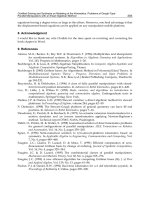
Rolland 2006]. Secondly, the typical spatial parallel manipulator is an hexapod constituted
by six kinematics chains and a sensor number corresponding to the actuator number,
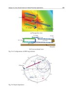
namely the 6-6 general manipulator, fig. 1.



Fig. 1. The general 6-6 hexapod manipulators
Solving the FKP of general parallel manipulators was identified as finding the real roots of a
system of non-linear equations with a finite number of complex roots. For the 3-RPR, 8
assembly modes were first counted, [Primerose and Freudenstein 1969]. Hunt geometrically
demonstrated that the 3-RPR could yield 6 assembly modes, [Hunt 1983]. The numeric
Parallel Manipulators, Towards New Applications

176
iteration methods such as the very popular Newton one were first implemented,
[Dieudonne 1972, Merlet 1987, Sugimoto 1987]. They only converge on one real root and the
method can even fail to compute it. To compute all the solutions, polynomial equations
were justified, [Gosselin and Angeles 1988]. Ronga, Lazard and Mourrain have established
that the general 6-6 hexapod FKP has 40 complex solutions using respectively Gröbner
bases, Chern classes of vector bundles and explicit elimination techniques, [Ronga and Vust
1992, Lazard 1993, Mourrain 1993a]. The continuation method was then applied to find the
solutions, [Raghavan 1993], however, it will be explained why they are prone to miss some
solutions, [Rolland 2003]. Computer algebra was then selected in order to manipulate exact
intermediate results and solve the issue of numeric instabilities related to round-off errors so
common with purely numerical methods. Using variable elimination, for the 3-RPR, 6
complex solutions were calculated [Gosselin 1994] and, for the 6-6, Husty and Wampler

applied resultants to solve the FKP with success, [Husty 1996, Wampler 96]. However,
resultant or dialytic elimination can add spurious solutions, [Rolland 2003] and it will be
demonstrated how these can be hidden in the polynomial leading coefficients. Inasmuch, a
sole univariate polynomial cannot be proven equivalent to a complete system of several
polynomials. Intervals analyses were also implemented with the Newton method to certify
results, [Didrit et al. 1998, Merlet 2004]. However, these methods are often plagued by the
usual Jacobian inversion problems and thus cannot guarantee to find solutions in all non-
singular instances. The geometric iterative method has shown promises, [Petuya et al. 2005],
but, as for any other iterative methods, it needs a proper initial guess.
Hence, this justified the implementation of an exact method based on proven variable
elimination leading to an equivalent system preserving original system properties. The
proposed method uses Gröbner bases and the rational univariate representation, [Faugère
1999, Rouillier 1999, Rouillier and Zimmermann 2001], implementing specific techniques in
the specific context of the FKP, [Rolland 2005]. Three journal articles have been covering this
question for the general planar and spatial manipulators [Rolland 2005, Rolland 2006,
Rolland 2007]. This algebraic method will be fully detailed in this chapter.
This document is divided into 3 main topics distributed into five sections. The first part
describes the kinematics fundamentals and definitions upon which the exact models are
built. The second section details the two models for the inverse kinematics problem,
addresses the issue of the kinematics modeling aimed at its adequate algebraic resolution.
The third section describes the ten formulations for the forward kinematics problem. They
are classified into two families: the displacement based models and position based ones. The
fourth section gives a brief description of the theoretical information about the selected exact
algebraic method. The method implements proven variable elimination and the algorithms
compute two important mathematical objects which shall be described: a Gröbner Basis and
the Rational Univariate Representation including a univariate equation. In the fifth section,
one FKP typical example shall be solved implementing the ten identified kinematics models.
Comparing the results, three kinematics models shall be retained. The selected manipulator
is a generic 6-6 in a realistic configuration, measured on a real parallel robot prototype
constructed from a theoretically singularity-free design. Further computation trials shall be

performed on the effective 6-6 and theoretical one to improve response times and result files
sizes. Consequently, the effective configuration does not feature the geometric properties
specified on the theoretical design. Hence, the FKP of theoretical designs shall be studied
and their kinematics results compared and analyzed. Moreover, the posture analysis or
assembly mode issue shall be covered.
Certified Solving and Synthesis on Modeling of the Kinematics. Problems of Gough-Type
Parallel Manipulators with an Exact Algebraic Method

177
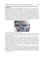
2. Kinematics of parallel manipulator
2.1 Kinematics notations and hypotheses



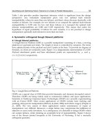
Fig. 2. Typical kinematics chains
The parallel Gough platform, namely 6-6, is constituted by six kinematics chains, fig. 2. It is
characterized by its mechanical configuration parameters and the joint variables. The
configuration parameters are thus OA
Rf
as the base geometry and CB
Rm
as the mobile
platform geometry. The joint variables are described as ρ the joint actuator positions
(angular or linear). Lets assume rigid kinematics chains, a rigid mobile platform, a rigid base
and frictionless ball joints between platforms and kinematics chains.
2.2 Hexapod exact modeling
Stringent applications such as milling or surgery require kinematics models as close as
possible to exactness. Realistically, any effective configuration always comprises small but
significant manufacturing errors, [Vischer 1996, Patel & Ehmann 1997]. Hence, any
constructed parallel manipulator never corresponds to the theoretical one where specific

geometric properties may have been chosen, for example, to alleviate singularities or to
simplify kinematics solving. Two prismatic actuator axes may be neither collinear nor
parallel and may not even intersect. Whilst knowing joints prone to many imperfections,
then rotation axes are not intersecting and the angles between them are never
perpendicular. Moreover, real ball joints differ from a perfectly circular shape and friction
induces unforeseeable joint shape modification, which results into unknown axis changes.
However, the joint axis angles stay almost perpendicular and any rotation combination shall
be feasible. In a similar fashion, the Cardan joint axes are not perpendicular and may be
separated by a small offset. Finally, the articulation center is not crossed by any axis.
Identified the hexapode 138, the exact geometric model is then characterized by 138
configuration parameters. Each kinematics chain is described by 23 parameters, as shown on
fig. 2 and defined hereafter:
• the 3 parameters of each base joint A
i
with their error vector δA
i
,
• the 3 joint Ai inter-axis distances є
1
a
,

є
2
a
and є
3
a

• each prismatic joint measured position l

i
with its error coordinate δL
i
,
• the 3 parameters of the minimum distance between the two prismatic actuator axes:
r
d

,
• the angular deviation between the two prismatic actuator axes: φ,
• the 3 parameters of the platform joint B
i
with their error vector δB
i
,
• the 3 joint B
i
inter-axis distances and є
1
b
, є
2
b
and є
3
b

Parallel Manipulators, Towards New Applications

178

To solve this model includes the determination of parameters which cannot be measured
neither determined. Moreover, the model includes more variables than equations and
therefore, its resolution would then only be possible through optimization methods. Relying
on a calibration procedure would only determine configuration parameters by specifying an
error margin consisting of a radius around joint positions and would not indicate the
direction of the error vector. Hence, only an error ball becomes applicable to the model. In
practice, the δA
i
and δB
i
joint error vectors shall reposition the respective kinematics chains
by adding an offset to the joint centers. Thus, a random function shall compute the δA
i
and
δB
i
vectors with the maximum being the error ball radius. Finally, the selected model,
namely the hexapod 84, is effectively based on the hexapod 42 model with errors added to the
configuration data and joint variables.
2.3 Kinematics problems
Definition 2.1 The kinematics model is an implicit relation between the configuration parameters
and the posture variables, F( X

, Γ, OA
|Rf
,CB
|Rm
)=0 where
Γ
= {

ρ
1
,
ρ
2
,…,
ρ
6
}.



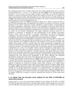
Fig. 3. Kinematics model
Three problems can be derived from the above relation: the forward kinematics problem
(FKP), the inverse kinematics problem (IKP) and the kinematics calibration problem, fig. 3.
The two first problems shall be covered in this article. The inverse kinematics problem (IKP)
is defined as:
Definition 2.2 Given the generalized coordinates of the manipulator end-effector, find the joint
positions.
The 6-6 IKP yields explicit solutions from vector
Γ
= G(
X

, OA
|R f
, CB
|Rm
) and is used to
prepare the FKP which is defined as:

Definition 2.3 Given the joint positions
Γ
, find the generalized coordinates X

of the manipulator
end-effector.
The 6-6 FKP is a difficult problem, [Merlet 1994, Raghavan and Roth 1995] and explicit
solutions
X

= G(
Γ
, OA
|R f
, CB
|Rm
) have not yet been established. The difficulties in solving
the FKP have hampered the application of parallel robot in the milling industry.
Certified Solving and Synthesis on Modeling of the Kinematics. Problems of Gough-Type
Parallel Manipulators with an Exact Algebraic Method

179
2.4 Vectorial formulation of the basic kinematics model


Fig 4. The vectorial formulation
The vectorial formulation produces an equation system which contains the same number of
equations as the number of variables, fig. (4), [Dieudonne et al. 1972]. A closed vector cycle
is constituted between the manipulator characteristic points: A
i

and B
i
, kinematics chain
attachment points, O the fixed base reference frame and C the mobile platform reference
frame. For each kinematics chain, a function between points A
i
and B
i
expresses the
generalized coordinates X, such as
ii
A
B


= U
1
(X). Inasmuch, vector
ii
A
B


is determined with
the joint coordinates
Γ
and X giving a function U
2
(X,
Γ

). Finally, the following equality has
to be solved: U
1
(X) = U
2
(X,
Γ
).
3. The inverse kinematics problem
For each kinematics chain, i = 1, , 6, each platform point
|iRf
OB


can be expressed in terms of
the distance constraint, [Merlet 1997]:

6 1,
2
2
== i
BA
l
ii
i
(1)
Using the vectorial formulation, two equation families can be derived: displacement-based
and position-based equations.
3.1 Displacement based equations
Any mobile platform position

|
OB
R
f


which meets constraints 1 has a rotation matrix ℜ such
that:
|| |
,16
ff m
iR iR iR
OB OC CB i=+ℜ⋅ =

 
…
(2)
Parallel Manipulators, Towards New Applications

180
Substituting 2 in 1, we obtain:

2
2
|||
,16
fmf
RiRiR
i
lOC CB OA i=+ℜ⋅− =


  
…
(3)
This last equation system can be developed and simplified, leading to the IKP :

(
)
(
)
2
2
2
|| || |
ff ff m
R iR R iR iR i
i
lOCOA OCOA CB CB=− +−ℜ⋅+

    
(4)
3.2 Position based equations
In 3D space, any rigid body can be positioned by 3 of its distinct non-colinear points,
[Fischer and Daniel 1992, Lazard 1992b]. The 3 mobile platform distinct points are usually
selected as the 3 joint centers B
1
, B
2
, B
3

, fig. 5. The 6 variables are set as:
|iRf
OB


= [x
i
, y
i
, z
i
] for i
= 1 . . . 3. The
|iRf
OB


parameters define the reference frame R
b1
relative to the mobile
platform and B
1
is chosen as its center. The frame axes u
1
, u
2
and u
3
are determined by the 3
platform points:

1
13
2
12312
12 13
,,
BB
BB
uuuuu
BB BB
=
==∧





(5)
Any platform point M can be expressed by
1
BM


= a
M
u
1
+ b
M

u
2
+ c
M
u
3
where a
M
, b
M
, c
M
are
constants in terms of these three points. Hence, in the case of the IKP, the constants are
noted a
Bi
, b
Bi
, c
Bi
, i = i . . . 6 and can explicitly be deduced from CB
|Rm
by solving the
following linear system of equations:

1
1123
|
,16
iii

b
BBB
iR
BB a u b u c u i=++ =


…
(6)



Fig. 5. The platform three point coordinate system
Certified Solving and Synthesis on Modeling of the Kinematics. Problems of Gough-Type
Parallel Manipulators with an Exact Algebraic Method

181
Substituting relations 6 in the distance equations l
i
2
= ║
ii
A
B


|Rf
║, i = 1 . . . 6, the system can
be expressed with respect to the variables x
i
, y

i
, z
i
, i = 1, 2, 3. Thus, for i = 1 . . . 6, the IKP is
obtained by isolating the ρ
i
or l
i
linear actuator variables in the six following equations:

()
(
)
2
2
2
, 1 3
ii
ix iy
i
i
y
lx
OA OA
=− +− =

 
(7)

1

2
2
|
|
,46
b
f
kR
kR
i
lB OA i=− =


…
(8)
4. The forward kinematics problem
4.1 Displacement based equations
There exist various formulations of the displacement based equation models.
4.1.1 AFD1 - formulation with the position and the trigonometry identity
The AFD1 formulation is obtained by replacing each trigonometric function of the IKP
rotation matrix, 2, by one distinct variable, [Merlet 1987], for j = 1, 2, 3, then c
j
= cos(Θj), s
j
=
sin(Θ
j
). The end-effector position variables are retained. The 9 unknowns are then: {x
c
, y

c
, z
c
,
c
1
, c
2
, c
3
, s
1
, s
2
, s
3
}. The orientation variables can either be any Euler angles or the navigation
ones (pitch, yaw and roll). The orientation variables are linked by the 3 trigonometric
identities, for j = 1 . . . 3, then c
2
j
+ s
2
j
= 1 which complete the equation system:

(
)
(
)

2
2
|| || |
,1,,6
ff ff m
RiR RiR iR
i i
FOCOA OCOA CB Li=− +−ℜ⋅−=

    
…
(9)

22
1, 1,2,3
jjj
Fcs j=+− = (10)
The system is constituted of 9 equations with 6 polynomials of degree 6 and 3 quadratics.
The model is simply build by variable substitution without any computation. Thus, the
coefficients remain unchanged. The number of variables is not minimal.
4.1.2 AFD2 - formulation with the position and the trigonometric function change
The end-effector position variables are retained. Rotation variable changes can apply the
following trigonometric relations, [Griffis & Duffy 1989, Parenti-Castelli & C. Innocenti 1990,
Lazard 1993]. For i = 1, 2, 3:

()
()
()
(
)

()
2
2
2
1
1
cos,
1
2
sin,
2
tan
i
i
i
i
i
i
i
i
t
t
t
t
t
+
−
=
+
=

⎟
⎠
⎞
⎜
⎝
⎛
=
θθ
θ
(11)
The 6 variables become {x
c
, y
c
, z
c
, t
1
, t
2
, t
3
}. The IKP equations (2) are rewritten to obtain the 6
following equations:

(
)
(
)
2

2
|| || |
,1,,6
ff ff m
RiR RiR iR
i i
FOCOA OCOA CB Li=− +−ℜ⋅−=

    
…
(12)
The final equation system comprises 6 equations of order 8 with the high degree monomial
being x
i
2
x
j
2
x
k
2
x
n
2
. This model has a minimal variable number. The polynomials coefficients
Parallel Manipulators, Towards New Applications

182
are expanding due to variable change computation. Moreover, this representation is not
intuitive.

4.1.3 AFD3 - formulation with the translation and rotation matrix
The intuitive way to set an algebraic equation system from the IKP equations 2 is to
straightforwardly use all the rotation matrix parameters and the vector
OC


|Rf
coordinates
as unknowns, [Lazard 1993, Sreenivasan et al. 1994, Bruyninckx and DeSchutter 1996]. The
variables are then {X
c
, Y
c
, Z
c
, r
ij
, j=1 3, i=1 3}. Since
ℜ
is a rotation matrix, the following
relations hold:
ℜ
t
ℜ
= Id or det(
ℜ
) = 1. These relations are redundant since
ℜ
t
ℜ

is
symmetrical and they generate the 7 following equations:

⎪
⎩
⎪
⎨
⎧
−++−−=
++=++=++=
++=++=++=
221331231231321321331221322311332211
332332223121331332123111231322122111
2
33
2
32
2
31
2
23
2
22
2
21
2
13
2
12
2

11
1
0,0,0
1,1,1
rrrrrrrrrrrrrrrrrr
rrrrrrrrrrrrrrrrrr
rrrrrrrrr
(13)
Six rotation matrix constraints are then selected and preferably with the lowest degree
polynomials. This leads to an algebraic system with 12 polynomial equations (13 and 1) in 12
unknowns.

(
)
(
)
2
2
|| || |
,1,,6
ff ff m
RiR RiR iR
i i
FOCOA OCOA CB Li=− +−ℜ⋅−=

    
…
(14)

1

2
13
2
12
2
117
−++= rrrF
(15)

1
2
23
2
22
2
218
−++= rrrF
(16)

1
2
33
2
32
2
319
−++= rrrF
(17)

23132212211110

rrrrrrF
+
+
=
(18)

33133212311111
rrrrrrF
+
+
=
(19)

33233222312112
rrrrrrF
+
+
=
(20)
Finally, the model polynomials are quadratic and minimal. They are obtained by
substitution and no computations are required. The coefficients are then unchanged. There
is a very large number of variables.
4.1.4 AFD4 - formulation with the translation and Gröbner Basis on the rotation matrix
The rotation matrix constraints are not depending on the end-effector position variables.
Hence, if one Gröbner Basis is computed from the rotation constraints, the Gröbner Basis is
also independent of the position variables and thus constant for any FKP pose. Therefore,
one preliminary Gröbner Basis can be calculated and saved into a file for later reuse.
Hence, the rotation matrix constraints in the system 20 can be replaced by their Gröbner Basis
comprising 24 equations where the coefficients are only unity. Thus, the algebraic system
involves 30 equations and 12 variables.

Certified Solving and Synthesis on Modeling of the Kinematics. Problems of Gough-Type
Parallel Manipulators with an Exact Algebraic Method

183
4.1.5 AFD5 - translation and quaternion algebraic model
Based on equation (2), quaternions can express mobile platform rotation, [Lazard 1993,
Mourrain 1993b, Egner 1996, Murray et al. 1997]. The quaternion representation includes 4
variables {q
0
; q
1
; q
2
; q
3
} where the vector q = q
1
i +q
2
j +q
3
k defines the platform specific
rotation axis and q
0
= cos(α/2) determines the coordinate expressing the rotation
α
along
that axis. Thus, the rotation matrix
ℜ
used in equations 4 may then be expressed in terms of

the quaternion coordinates and with Δ
2
= q
0
2
+ q
1
2
+ q
2
2
+ q
3
2
, we can write:

(
)
(
)
() ()
()()
2222
0123 1203 1302
2
2222
1203 0123 2301
2222
13 02 23 01 0 1 2 3
22

22
22
qqqq qqqq qqqq
qq qq q q q q qq qq
qq qq qq qq q q q q
−
⎛⎞
+−− − +
⎜⎟
ℜ= + − + − −
⎜⎟
⎜⎟
−+−−+
⎝⎠
Δ
(21)
The end-effector position variables are retained. Moreover, one may implement a unitary
quaternion: Δ
2
= 1. Rewriting the IKP equations 4, we obtain 7 polynomial equations in the 7
unknowns {X
c
; Y
c
; Z
c
; q
0
; q
1

; q
2
; q
3
}:

(
)
(
)
2
2
|| || |
,1,,6
ff ff m
RiR RiR iR
i i
FOCOA OCOA CB Li=− +−ℜ⋅−=

    
…
(22)

2222
70123
1Fqqqq
=
+++−
(23)
The system contains 6 polynomials of degree 6 and 1 quadratic. The highest degree

monomial is x
i
2
x
j
2
. The quaternion has intrinsic coordinate redundancy which allows
avoiding typical mathematical singularities seen in other representations. The number of
variable is almost minimal. The rotation matrix system must be recomputed leading to
larger resulting polynomial coefficients.
4.1.6 AFD6 - translation and dual quaternion algebraic model
Not only orientations can be formulated using quaternions, but also positions, [Husty 1996,
Wampler 96]. The
ℜ
rotation matrix is then expressed in terms of the first quaternion
Φ
=
{
c
0
;
c
1
; c
2
; c
3
}
. In a sense, the second
Ψ

=
{
g
1
, g
2
, g
3
, g
4
}
represents the end-effector position.
Moreover, one relation can be written between the two quaternions:
Φ
= OC
Ψ
. This relation
unfolds in the following equations from which two constraint equations, noted FC
1
= 0 and
FC
2
= 0, are selected. Lets s
i
= OA
|Rf
and t
i
= CB
|Rm

, then:

1
1
0
0
20
t
t
tt
tt
ii
cc
gc
gg lcc
csc gtc
=
=
−=
+
=
For i = 2,…,6 (24)
The dual quaternion system is thus constituted by the 8 following equations, for i = 1 … 6 :

(
)
(
)
2
2

|| || |
ff ff m
R iR R iR iR
i i
FOCOA OCOA CB L
=
−+−ℜ⋅−

    
(25)

17
FCF
=
(26)
Parallel Manipulators, Towards New Applications

184

28
FCF
=
(27)
The system comprises 6 polynomials of degree 4 and 2 quadratics. The highest degree
monomials are either x
i
4
; x
i
3

x
j
or x
i
2
x
j
2
. One more variable is added over the former
quaternion model. The variable choice is not intuitive.
4.2 Position based equations
We shall examine four formulations derived from the position based equations. Every
variable has the same units and their range is equivalent.
4.2.1 AFP1 - three point model with platform dimensional constraints
The 3 platform distinct points are usually selected as the three joint centers B
1
, B
2
and B
3
, fig.
5. The 6 variables are set as: OB


i|Rf
= [x
i
, y
i
, z

i
] for i = 1 …3.
Using the relations 6, the constraint equations L
i
2
= ║
ii
A
B


|Rf
║
2
, i = 1, …, 6 can be expressed
with respect to the variables x
i
, y
i
, z
i
, i = 1, 2, 3. Together with equations 30, they define an
algebraic system with 9 equations in 9 unknowns {x
1
, y
1,
z
1
, x
2

, y
2
, z
2
, x
3
, y
3
, z
3
}. The resulting
kinematics chain system becomes:

(
)
(
)
(
)
3 1,
2
222
=−−+−+−= iLOAxOAyOAxF
iixiiyiixii
(28)

1
2
2
|

|
,46
b
f
jR
jR
jj
FB OA Lj=− −=


…
(29)
The mobile platform geometry yields the following three distance equations:

()()()
()()()
()()()
2
|2
3
2
23
2
23
2
23
2
|2
39
2

|1
3
2
13
2
13
2
13
2
|1
38
2
|1
2
2
12
2
12
2
12
2
|1
27
mf
mf
mf
RR
RR
RR
BBzzyyxxBBF

BBzzyyxxBBF
BBzzyyxxBBF
=−+−+−−=
=−+−+−−=
=−+−+−−=
(30)
Together with equations 30, they produce an algebraic system with 9 equations with 9
unknowns {x
1
, y
1
, z
1
, x
2
, y
2
, z
2
, x
3
, y
3
, z
3
}. In all instances, it can be easily proven that this 6-6
FKP formulation yields 9 quadratic polynomials.
The system variable choice is relatively intuitive. Each equation polynomial is always
quadratic. However, the b
1

reference frame and the platform points B
i
in the b
1
frame require
computations, which usually result into coefficient size explosion. The variable number is
not minimal.
4.2.2 AFP2 - the three point model with platform constraints
The former system can be slightly modified by replacing the last mobile platform constraint
with a platform normal vector one. Hence, lets take the two mobile platform vectors
12
BB

and
13
BB

, then the last constraint is calculated from these two vector multiplication:
Certified Solving and Synthesis on Modeling of the Kinematics. Problems of Gough-Type
Parallel Manipulators with an Exact Algebraic Method

185

()()()
()()()
()()()( )()()
mm
mf
mf
RR

RR
RR
BBBBzzzzyyyyxxxxF
BBzzyyxxBBF
BBzzyyxxBBF
|1
3
|2
31213121312139
2
|1
3
2
13
2
13
2
13
2
|1
38
2
|1
2
2
12
2
12
2
12

2
|1
27
∧−−∗−+−∗−+−∗−=
=−+−+−−=
=−+−+−−=
(31)
The result is still an algebraic system with nine equations in the former nine unknowns
{x
1
, y
1
, z
1
, x
2
, y
2
, z
2
, x
3
, y
3
, z
3
}. The 6-6 FKP formulation using this three point model is
constituted by nine quadratic polynomials.
4.2.3 AFP3 - the three point model with constraints and function recombination
By rewriting the IKP as functions, the algebraic system comprises three equations and three

functions in terms of the nine variables: x
1
, y
1
, z
1
, x
2
, y
2
, z
2
, x
3
, y
3
, z
3
, equation (29).

(
)
(
)
3 1,
2
22
=−−+−= ilOAyOAxF
iiyiixii
(32)

1
2
2
|
|
,46
b
f
kR
kR
ii
CB OA li=− −=

 
…
(33)
Hence, three constraints are derived from the following three functions, [Faugère and
Lazard 1995]. Two functions can be written using two characteristic platform vector norms
between the B
1
,B
2
distinct points and the B
1
,B
3
ones. The last function comes from these
vector multiplication.

()()()
()()()
()()()( )()()
mm
mf
mf
RR
RR
RR
BBBBzzzzyyyyxxxxF
BBzzyyxxBBF
BBzzyyxxBBF
|1
3
|2
31213121312139
2
|1
3
2
13
2
13
2
13
2
|1
38
2
|1

2
2
12
2
12
2
12
2
|1
27
∧−−∗−+−∗−+−∗−=
=−+−+−−=
=−+−+−−=
(34)
Furthermore, the three last equations (F
7
, F
8
, F
9
) are computed by the following function
sequential combinations:
F
7
= −C
7
+ F
1
+ F
2

F
8
= −C
8
+ F
1
+ F
3
(35)
F
9
= 2∗C
9
+ F
7
+ F
8
− 2∗ F
1

The formulation is completed with other function combinations obtained by the following
algorithm leading to three middle equations (F
4,
F
5
, F
6
). Let d
7
= ║

21
BB


|Rmj
║, d
8
=
║
31
BB

|Rm
║
2
and d
9
= ║
32
BB


|Rm║ ^ ║
31
BB


|Rm
║, then for i = 4, 5, 6, we compute:

(
)
(
)
()( )
() ()
()
()
iiii
ii
ii
iiiii
BB
i
BBB
BBii
BBii
BBBBBii
bFaFFbaFFFFdc
FFFdcFFFdcCF
FFFbFFaCC
CbaCCCcCbCaCC
∗−∗−∗−+∗+∗−+−∗∗∗−
−+∗∗∗−−+∗∗∗−=
−+∗−∗−∗−∗=
∗∗∗−−∗∗−∗−∗−=
87118979
2
7218

2
8217
2
72117
9
2
987
2
8
2
7
2
1222
22
22
2
(36)
Parallel Manipulators, Towards New Applications

186
The result is an algebraic system with nine equations with the nine unknowns. The 6-6 FKP
formulation using this modified three point model includes six quadratic and three quartic
polynomials. The system includes polynomials of higher degree than for the former two
position based models. Computations cause to coefficient expansion.
4.2.4 AFP4 - the six point model
The six mobile platform B
i
joints can be used in defining 18 variables, [Rolland 2003]. Taking
the IKP equations (8), a position based variation is obtained:

(
)
(
)
(
)
6 1,
222
2
=−+−+−= iOAxOAyOAxl
ixiiyiixii
(37)
The system is completed with 12 distance constraint equations selected among the distinct B
i

passive platform joints. Here are some examples:

()()()
()()()
()()()
64,
63,
61,
2
|3
2
3
2
3
2

3
2
|3
2
|2
2
2
2
2
2
2
2
|2
2
|1
2
1
2
1
2
1
2
|1
…
…
…
==−+−+−=
==−+−+−=
==−+−+−=
kBBzzyyxxBB

jBBzzyyxxBB
iBBzzyyxxBB
mf
mf
mf
R
kkkk
R
k
R
jjjj
R
j
R
iiii
R
i
(38)
The formulation results in 18 polynomials in the 18 unknowns:
{x
1
, y
1
, z
1
, x
2
, y
2
, z

2
, x
3
, y
3
, z
3
, x
4
, y
4
, z
4
, x
5
, y
5
, z
5
, x
6
, y
6
, z
6
}. The system is then constituted of
quadratic polynomials. This variable choice is intuitive and the system yields minimal
degree. Finally, the number of variables is maximal.
5. Solving polynomial systems using exact computation
5.1 Mathematical system solving

Kinematics problems contain systems of several equations containing non-linear functions
with various variable numbers. These systems can be difficult to solve, especially in the
general 6-6 cases and response times actually makes them inappropriate for
implementations in design, simulation or control. In some instances, the results may appear
to be faulty bringing doubts to the reliability of the methods.
If left without any reliable and performing methods, the tendency, in engineering practice,
would be to convert the difficult models into simpler linearized ones. In material handling,
this proposal might suffice, however, in high speed milling where the accuracy
requirements are more severe, any simplification can have a dramatic impact, whereby
result certification becomes an important issue.
However, with proper polynomial formulation, algebraic methods can lead to at least
certified and even exact results, whereas numeric methods, unless they implement proper
interval analysis, cannot actually obtain certified results since they are prone to numeric
instabilities or matrix inversion problems. Therefore, although time consuming, algebraic
methods are preferred since they handle integer, rational and symbolic values as such
without any truncation or approximation, even when manipulating intermediate results.
Hence, there will be no loss of information.
Certified Solving and Synthesis on Modeling of the Kinematics. Problems of Gough-Type
Parallel Manipulators with an Exact Algebraic Method

187
Solving non-linear equation systems will usually result in several complex solutions, out of
which a certain subset are real solutions. However, only the real solutions bear practical
significance, since they correspond to effective manipulator poses.
5.2 Calculation accuracies
The calculation accuracies are depending upon the type of arithmetic, the behavior of the
calculation methods and the quality of the implemented algorithms.
Definition 5.1 An exact calculation is defined as a calculation which always produces the same exact
result to the same specific mathematical problem.
The result does not contain any error. Its representation is also exact.

Definition 5.2 A reliable computation is defined as one which will always give the same result from
the same initial input data presented in the same format.
Definition 5.3 A certified calculation is defined as a reliable computation giving a result distant
from the true solution by a certain maximum known accuracy.
Hence, such a calculation may not be exact. However, the result contains some exact digits.
Hence, we shall try to apply a method that computes certified results and if possible exact
ones.
For example, lets take the univariate function f
1
(x) = x
2
− 4/25. Computing f
1
= 0, we obtain
the exact response: {−2/5, 2/5}. The closed-form resolution calculates exact results with
rational numbers. Therefore, the result is certified without any error.
Lets consider f
2
(x) = x
2
− 5. Solving f
2
= 0, the result will be two irrational numbers which can
only be represented by truncation. However an interval can be certified to contain the exact
result: {[2, 5/2], [−5/2, 2]}. Wherefore, exact computations keep intermediate results in
symbolic format whenever possible and only revert to rational or floating boundary
numbers for display purposes.
Therefore, any real number can be coded by an interval which width corresponds to the
required accuracy. However, the difficulty lies in insuring that the interval contains the
exact result which is not known a priori.

Fig. 6. Bloc Diagram of the Continuation Method
5.3 Solving a non-linear system
Two method groups have been advocated to find all solutions of the FKP, namely:
continuation methods and variable elimination ones, [Raghavan and Roth 1995]. The first
approach is usually realized in a numeric environment and the later algebraic.
Parallel Manipulators, Towards New Applications

188
5.4 Continuation method with homothopy
In order to compute several solutions, the continuation method can be implemented with a
homothopy process. The Continuation approach implements a numerical iterative method
which is successively repeated in order to progressively transfer from an original equation
system which solutions are predetermined to another system relatively close to the former,
Fig. 6.
Let a system of equation be F(X) = 0 with variables X = {x
1
,…,x
n
}; we wish to find the
solution to this equation system. Let G(X) = 0 be a similar equation system which roots are
already known, namely the variety Vr (I)
G
; then, we set the continuation process as H(X, λ) =
G(X)+ λ (F(X)−G(X)) and commence with λ = 0. It provides for a mechanism to convert an
original equation system into a final one through several steps. At each step, H(X, λ) is
successively computed with a new value of λ which is increased by a small arbitrary
increment δλ such that λ ∈ {0,…, 1}. The homothopy principle assumes connectivity between
solutions of each system computed with the various λ. More generally, if the system H(X, λ)

with λ as a variable would be solved, it would result in paths as solutions.




Fig. 7. Examples of path following with the Continuation Method
The continuation method cannot solve any equation system as such and, at each step, when
λ is instanciated, the H(X, λ) system roots are computed by a typical iterative method, either
the Newton one or the new Geometric Iterative Method which is a potentially good alternative,
[Petuya et al. 2005].
This method was first applied to classical robotics kinematics, [Tsai & Morgan 1984] and
then applied to solve the parallel manipulator FKP, [Kholi et al. 1992, Sreenivasan and P.
Nanua 1992].
Advocating that a little change on parameters of one system shall cause only a small change
on solutions, the continuation method could be used to find the 40 solutions on some 6-6
FKP cases, [Raghavan 1993].
It is feasible to construct an efficient and reliable method; however, the method is still
unproven. Moreover, continuation does not alleviate the problems related to the application
of a numeric iterative method.
Certified Solving and Synthesis on Modeling of the Kinematics. Problems of Gough-Type
Parallel Manipulators with an Exact Algebraic Method

189
This method can be somewhat delicate to implement. There exist several scenarios which
might pose significant problems depending on how the solution paths evolve from λ = 0 to λ
= 1, see fig. 7, where solutions:
- go to or come from infinity,
- merge or split,
- start complex and become real,
- start real and become complex.

Therefore, proper implementation would require a priori continuation process verification
which is still an open question, since this would require solving a one-dimensional system
H(X,λ) where λ is left as a variable and this is an even more difficult problem. Inasmuch, in
many instances, finding a nearby equation system with known roots may not be always be
feasible. Then, there is also an issue on what constitutes a sufficiently similar system.
However, it is very difficult to determine precisely what the meaning of sufficiently similar
is.
5.5 Variable elimination
5.5.1 Introduction
Most algebraic methods which were implemented to solve the parallel manipulator FKP
apply one form of variable elimination. Let an algebraic system F(X) = 0 be a system of
polynomial functions f
i
(X), i = 1,…,m with variables X = {x
1
,…,x
n
}, the variable elimination
approach consists in the transformation of the original system F(X) = 0 into another system
H(Y) = 0 with functions g
j
(X), j = 1,…,p with variables Y = {y
1
,…,y
r
} where r < n. Ultimately,
the goal is to find a method which allows to compute an equation system H(Y) in either
triangular format or preferably in univariate form which would be the easiest to solve.
Most variable elimination methods are usually divided into four steps:
- Step 1: Variable elimination.

- Step 2: Solving the univariate equation.
- Step 3: Return or extension to original system variables.
We will examine the variable elimination methods which were successfully applied to solve
the FKP from which two can be identified:
- method based on resultant calculation including the so-called dialytic elimination,
- method based on Gröbner basis calculation.
5.5.2 Resultant method
Variable elimination can be implemented through a recursive method based on resultants.
As input, we give a system of equations with rational coefficients. The output will be one
univariate polynomial equation in terms of one of the original variables. Each elimination
step involves two polynomial equations which results in one equation with the number of
variable reduced by one.
Definition 5.4 [Cox et al. 1992] Let a system be F(X) = {f1,…,fn}
∈
Q[x1, … , xn]; let P = fi and
R = fj where fi = apx1p +…+a0 and fj = bqx1q +…+bq with i, j
∈
{1, 2,…,n} and ai, bi
∈

Q[x2,…,xn], let p = deg(P) et r = deg(R) knowing that p, r
∈
N* ; suppose that a0
≠
0 and b0
≠
0 ;
then Res(f, g, x1) = det(M) which is the resultant of P and R in terms of x1 where M is the identified
as the Sylvester matrix.
Then, the Sylvester matrix can be expressed in terms of the polynomial coefficients:

Parallel Manipulators, Towards New Applications

190

⎟
⎟
⎟
⎟
⎟
⎟
⎟
⎟
⎟
⎠
⎞
⎜
⎜
⎜
⎜
⎜
⎜
⎜
⎜
⎜
⎝
⎛
=
1
22
11

0101
00
00
00
00
0000
ba
bbaa
bbaa
bbaa
ba
M
l
ml
ml







(39)
Inasmuch, we can write: Res(P, R, x
1
) = det(Sylv(P, R, x
1
). If we examine the Sylvester matrix,
we can observe that part with the a
i

parameters contains m columns and the one with b
i
n
columns.The following proposition holds and its proof is described in [Cox et al. 1992]: The
resultant Res(f, g, x) is the first ideal of elimination < f, g > ∩ k[x
2
,…,x
n
]; moreover, Res(f, g, x) = 0
iff f, g have a common factor in k[x
1
,…,x
n
] which has a positive degree in x. The nature of this
factor has to be determined and we wish to establish if it is only one root of functions f and
g. To answer that question, the following corollary will be employed: If f, g ∈ C[X] then Res(f,
g, x) = 0 iff f and g contain a common root in C. This common root is determined by computing
det(Sylv(P, R, x
1
) = 0. The nature of this root has to be determined, notably if it is a partial
one and the answer will come from the following proposition, [Cox et al. 1992] : Knowing
that f, g ∈ C[X], let a
0
, b
0

≠
0 and a
0
, b

0
∈ C[x
2
,…, x
n
], if Res(f, g, x) ∈ C[x
2
,…,x
n
] cancels at
(c
2
,…,c
n
), then we obtain that either a
0
b
0
= 0 at (c
2
,…,c
n
) or either ∃ c
1
∈ C such as f and g cancel.
In certain instances, the head terms of the polynomials can cancel which will result in the
cancellation of the determinant and the process consequently adds one extraneous root.
In order to obtain the univariate equation, a recursive algorithm will be applied. Firstly, we
calculate n − 1 resultants h
k

= Res(f
k+1
, f
1
, x
1
) on variable x
1
for k = 1,…,n − 1. Secondly, we
compute n − 2 resultants h
(
2)
j
= Res(h
j+1
, h
1
, x
2
) on variable x
2
for j = 1,…,n − 2 and we
continue in the same fashion until the univariate equation is determined. An almost
triangular equation system is constructed.

(
)
(
)
(

)
(
)
()()()
()
()
()
()
()
()
()
()
⎢
⎢
⎢
⎢
⎢
⎢
⎢
⎢
⎣
⎡
====
−
−
−
−
−
−−
−−

n
nn
n
nn
n
nnn
nnnnn
nnn
xH
xxhxxh
xxhxxh
xxhxxhxxh
XfXfXfXf
,,,
,,,,,,
,,,,,,,,,
0,0,0,,0
1
2
21
2
1
3
2
23
2
1
212221
121


………
…………
…
(40)
The last H(x
n
) is the targeted univariate equation. However, this equation cannot be
considered equivalent to the initial algebraic system because the head terms can cancel.
The return step to original variables is performed by substituting back through the
triangular system. The equation is solved H(x
n
) = 0 and we obtain a series of w roots {x
n
}. We
take the w roots, one by one, which is introduced in one of the equations h
1
(n
−
2)
(x
n
−1) = 0 or
h
2
(n
−
2)
(x
n
−1) = 0 and obtain the w roots {x

n
−1}. We continue until x
1
is isolated.
The 6-6 FKP has been solved applying resultants, [Husty 1996], in a computer algebra
environment to avoid intermediate result truncation, since, in a sense, parameter truncation
can be envisioned as changing the manipulator configuration.
Certified Solving and Synthesis on Modeling of the Kinematics. Problems of Gough-Type
Parallel Manipulators with an Exact Algebraic Method

191
A variation to the resultant method is called the dialytic elimination. Let the variable set be
X = {x
1
,…,x
n
} of the algebraic system F(X) = 0; then select any variable x
i
and set it as the
hidden variable, then a monomial vector is constructed around x
i
for the system F(X) which
is expressed as W = (1, x
i
, x
i
2
,…). The FKP is rewritten as a linear system in terms of W :

0=WA (41)

where :
W ≠ 0
Being a generalization of Res(P, Q, x
1
) = det(Sylv(P, Q, x
1
), it is subjected to the same risks of
root addition through the head term cancellation. Dialytic elimination has been
implemented to solve the FKP of the 3-RS or MSSM parallel manipulators, [Griffis and
Duffy 1989, Dedieu and Norton 1990, Innocenti and Parenti-Castelli 1990]. Satisfactory
results were produced on simple parallel manipulators, [Raghavan and Roth 1995].
5.6 Gröbner Bases
Lets denote by Q[x
1
,…,x
n
] the ring of polynomials with rational coefficients. For any n-uple
μ = (μ
1
,…, μ
n
) ∈ N
n
, lets denote by X
μ
the monomial X
1
μ
1
· · X

n
μ
n
. If < is an admissible
monomial ordering and
(
)
∑
=
=
r
i
i
i
XaP
0
μ
any polynomial in Q[X
1
, ,X
n
], the following
polynomial notations are necessary :
- LM(P,<) = max
i=0…r
, <X
μ
(i)
is the leading monomial of P for the order <,
- LC(P,<) = a

i
with i such that LT(P) = X
μ
(i)
is the leading coefficient of P for <,
- LT(P,<) = LC(P,<)· LM(P,<) is the leading term of P for <.
Lets denote by x
1
,…,x
n
the unknowns and S = {P
1
=,…,P
s
} any polynomial system as a subset
of Q[x
1
,…,x
n
]. A point α ∈ C
n
is a zero of S if P
i
(α) = 0 ∀i = 1…s. Actually, any large
polynomial equation system cannot be directly or explicitly solved. Thus, it is necessary to
revert to mathematical objects containing sufficient information for resolution. Any
polynomial system is then described by an ideal:
Definition 5.5 [Cox et al. 1992] An ideal I is defined as the set of all polynomial P(X) that can be
constructed by multiplying and adding all polynomials in the ring of polynomials with the original
polynomials in the set S.

A Gröbner Basis G is then as a computable polynomial generator set of a selected polynomial
set S = {P
1
,…,P
s
} with good algorithmic properties and defined with respect to a monomial
ordering. This basis is a mathematical object including the ideal I information. The
lexicographic and degree reverse lexicographic (DRL) orders are usually implemented, [Cox et
al. 1992, Geddes et al. 1994]. Given any admissible monomial ordering, the classical
Euclidean division can be extended to reduce a polynomial by another one in Q[X
1
,…,X
n
].
This polynomial reduction can be generalized to the reduction by a polynomial list. The
reduction output depends on the monomial ordering < and the polynomial order.
Definition 5.6 Given any admissible monomial ordering, <, a Gröbner Basis G with respect to < of
an ideal I
⊂
Q[X
1
,…,X
n
] is a finite subset of I such that:
∀
f
∈
I ,
∃
g

∈
G such that LM(g,<) divides
LM(f,<).
Some useful Gröbner Basis properties are described in the following theorem:
Theorem 5.1 Let G be a Gröbner Basis G of an ideal I
⊂
Q[X
1
,…,X
n
] for any < monomial ordering,
then a polynomial p
∈
Q[X
1
,…,X
n
] belongs to I if and only if the reduction algorithm Reduce (p, G,<
) = 0; the reduction does not depend on the order of the polynomials in the list of G; it can be used as a
simplification function.
Parallel Manipulators, Towards New Applications

192
The classical method for computing a Gröbner Basis is based on Buchberger's algorithm
[Buchberger et al. 1982, Buchberger 1985]. Recently, Faugère proposed more powerful
algorithms, namely accel and F4 implemented in the FGb software, [Faugère 1999].
5.7 Gröbner Bases and zero dimensional systems
Definition 5.7 [Lazard 1992a] A zero-dimensional system is defined as a mathematical equation
system with a variety (solution set) constituted by a finite number of complex points.
From a mathematical point of view, any variety is a valid result. From an engineering one,

we seek a variety which represents an exploitable result. For any parallel manipulator FKP,
the zero-dimensional systems allow pose analysis, since each real solution corresponds to each
manipulator pose. Otherwise the problems fall in the category of rarely usable singular
configurations. Detection of zero-dimensional systems is performed by implementing the
following theorem:
Theorem 5.2 Let G = {g
1
,…,g
l
} be a Gröbner Basis for any ordering < of any system S = {P
1
,…, P
s
}
∈
Q[X
1
,…,X
n
]
s
. The two following properties are equivalent:
- For all index i, i = 1…n, there exists a polynomial g
j

∈
G and a positive integer n
j
such that
X

i
nj
= LM(g
j
,<);
- The system {P
1
= 0,…,P
s
= 0} has a finite number of solutions in C
n
.
Hence, one can determine if the FKP resolution yields a finite or infinite number of
solutions. This is obviously an important issue, since an algebraic system with an infinite
number of solutions (variety of degree one or higher) cannot be directly exploited by a
control system and failure is usually the outcome.
5.8 The lexicographic Gröbner Basis
The choice of the monomial ordering is critical for the Gröbner Basis computation efficiency,
which is evaluated by the computation times, the size and the shape of the result. A
lexicographic Gröbner Basis with X
1
< X
2
< … < X
n
as variable order has always the following
general shape:

(
)

(
)
() ( )
()
()
⎪
⎪
⎩
⎪
⎪
⎨
⎧
=
=
==
==
+
+
−
0,,
,0,,
,0,,,0,
,0,,0
1
11
321121
21211
1
2
2

nk
nk
k
k
XXf
XXf
XXXfXXf
XXfXf
n
n
…
……
…
…
(42)
Whilst computing a lexicographic Gröbner Basis using Buchberger's algorithm yields doubly
exponential complexity in the worst case, an order change will save computation time.
Therefore, one DRL Gröbner Basis may first be computed in d
n
polynomial time where d is
the maximum total degree of the equations. Then, the DRL Gröbner Basis can be converted
into a lexicographic one in O(nD
3
) arithmetic operations, [Faugère et al. 1991]. In the case of
any zero-dimensional system, this can be done using exclusively linear algebra techniques,
[Faugère et al. 1991].
Definition 5.8 Let S be a system constituted by the polynomials p1,…,p
s

∈

Q[x
1
,…,x
n
], without
square factors. Let G = {g
1
,…,g
l
} be a Gröbner Basis computed for any ordering < on the system S. If
the univariate polynomial f(x
1
) is without any multiple factors, then the equation is square-free, the
first coordinates of all solutions are distinct and the solutions yield no multiple root. Then, the system
is considered in Shape Position .
Certified Solving and Synthesis on Modeling of the Kinematics. Problems of Gough-Type
Parallel Manipulators with an Exact Algebraic Method

193
If the polynomial system is in Shape Position, the Gröbner Basis has the following
simplified univariate format:
f
1
(X
1
) = 0, X
2
= f
2
(X

1
) = 0,…, X
n
= f
n
(X
1
) (43)
In this format, the lexicographic Gröbner Basis can be computed directly using the F4
algorithm, [Faugère 1999].
5.9 The rational univariate representation
Another root representation is given by the Rational Univariate Representation, hereafter
identified Rational Univariate Representation, [Rouillier 1999]. In the particular case of systems
in Shape Position, the univariate variable is the first one in the original system ones, so that
the Rational Univariate Representation can be written in the following format:

(
)
(
)
(
)
(
)
{
(
)
22 0 0
0, / , , /
kkknnkk

hX X h X h X X h X h X== =…
(44)


Fig. 8. The correspondence between the Rational Univariate Representation and original
system varieties.
h(X
k
) where 1 ≤ k ≤ n denotes the univariate equation, h
i
i = 0 … n the univariate return
functions. These polynomials are elements of Q[X
k
]. Inasmuch, h and h
0
are coprime.
Moreover, if the Rational Univariate Representation system is in Shape Position and if h(X
k
) is
square-free, the Rational Univariate Representation can be converted into a lexicographic
Gröbner Basis and the Rational Univariate Representation expression can be simply computed
from this basis. This situation is generally the case in most FKP instantiations:
h(X
k
) = f(X
k
), g(X
k
) = f
′

(X
k
) (45)
Moreover, since f and f
0
are coprimes, f
0
is invertible modulo f; this leads to: h
i
= f
i
⋅ (f
′
)
−
1

modulo f , i = 2 … n.
Definition 5.9 Let S be a system constituted by the polynomials p1,…, p
s

∈
Q[x
1
,…,x
n
] and let
G = {g
1
,…,g

l
} be a Gröbner Basis for any ordering < of the system S. Then, the RR form is defined as
the system R = {p
1
, p
1
−
1
p
2
mod G, p
1
−
1
p
3
mod G,…, p
1
−
1
pk mod G}
∈
Q[x
1
,…,x
n
] where p
1
−
1

is
calculated such that (p1 p
1
−
1
modulo G) = 1.
Parallel Manipulators, Towards New Applications

194
The rationale behind the RR form computation is to reduce the polynomial system S. The
computed Gröbner Basis G on any ordering < of the system S is used for the system
reduction. Then, the reduced system R resolution shall be less difficult.
Definition 5.10 Let S be a system constituted by the polynomials p
1
,…,p
s

∈
Q[x
1
,…, x
n
], if the
system S is without square factors and in Shape Position and if a lexicographic Gröbner Basis is
computable, then the system RR form R
′
can be deduced.
Since the S system reduction by a lexicographic Gröbner Basis leads to a further reduced
system R, one can conjecture faster FKP resolution. However, in some instances, p
1

−
1
can
hardly be computed and the RR form cannot be deduced. Hence, the FKP is solved by first
computing a Gröbner Basis on a DRL order and then we rely on the aforementioned order
change to obtain a lexicographic Gröbner Basis. In the rare instances where the FKP system is
not in Shape Position and a lexicographic Gröbner Basis is not computable either by the RR
form or by order change, the Rational Univariate Representation can be always be computed
by reverting to the more robust and lengthy algorithm taking as input any monomial
ordering Gröbner Basis and calculating the multiplication tables and matrices, [Rouillier
1999].
In practice, the Rational Univariate Representation coefficients are smaller than the
lexicographic Gröbner Basis ones, [Alonso et al. 1996]. This is the rationale behind the
preference of the Rational Univariate Representation expression which can be computed using
the algorithm described in [Rouillier 1999]. Anyhow, it should be deduced from a
lexicographic Gröbner Basis if the system is in Shape Position. Hence, in any case, the
determination of a lexicographic Gröbner Basis is first tried and then, a Rational Univariate
Representation is computed. In fact, for any parallel manipulator FKP, the computation of the
RR form is preferred. Finally, the method insures that the Rational Univariate Representation
system is equivalent to the former polynomial system. Each Rational Univariate
Representation system solution corresponds to one and only one original system solution and
the properties are preserved, fig. 8.
5.10 Real roots isolation
Once the Rational Univariate Representation is computed, then the real roots of the univariate
equation h(X
k
) roots can be isolated either using rapid numeric methods or exact algebraic
methods. As far as algebra is concerned, such computations can be performed by a method
such as the Uspensky one based on Descartes' sign rule and Sturm's theorem. An improved
algorithm is introduced in [Rouillier and Zimmermann 2001] applying one Vincent theorem.

In computer algebra and in particular in the proposed method, a natural way for coding a
real algebraic number
α
is given by either a square-free polynomial f with rational
coefficients such that f(
α
) = 0 or an interval [l,r] with rational bounds containing
α
.
Inasmuch, if
β
≠
α
and f(
β
) = 0 then
β
∉ [l, r].
Let
α
be a root of h(T) represented by ( h , [l, r]), then the resolution of h(T) = 0 produces a
solution list {
α
1,…,
α
r
} = [( h , [l
i
, r
i

]), i = 1 … r] where h is the square-free part of h.
Moreover, it is very easy to refine the intervals [l
i
, r
i
] by dichotomy since h is square-free
which induce that sign(
h (l
i
)) ≠ sign( h (r
i
)) if l
i
≠ r
i
.
Since h and h
0
are coprime by definition of the Rational Univariate Representation, one can
refine [l, r] so that it doesn't contain any real root of G. One can then simply use interval
arithmetic to compute [l
(i)
, r
(i)
] = h
i/
h
0
([l, r]); i = 1 … n. The complete method allows one
solution of the equation h(T) = 0 to correspond to each solution of the system F(X) = 0 since

the bijection is guaranteed and the properties are preserved, fig. 8.
Certified Solving and Synthesis on Modeling of the Kinematics. Problems of Gough-Type
Parallel Manipulators with an Exact Algebraic Method

195
Then, using the return functions h
i
/h
0
, for each
α
, we compute an interval product
() ()
[
]
iin
i
rl ,
0=
Π
containing [ h
1
/h
0
(
α
),…, h
n/
h
0

(
α
)]. For refining
(
)
(
)
[
]
iin
i
rl ,
0=
Π
, it is sufficient to
refine and introduce again [l, r] in the coordinate functions hi/h0; i = 1 … n.
The Rational Univariate Representation system real root isolation requires a second step where
the original system roots are determinated in terms of the original variables using the return
functions provided by the Rational Univariate Representation .
By computing a Rational Univariate Representation and then isolating the real roots as
described above, we obtain an exact method for isolating all the real roots of any polynomial
system with a finite number of complex roots verified during the computations using
theorem 5.2. The Rational Univariate Representation has rational coefficients and the isolating
intervals have rational bounds. For each solution
α
= (
α
1,…,
α
n

), the method produces :
- a box B
α
(
)
(
)
[
]
iin
i
rl ,
0=
Π
∈ R
n
such that
α
∈ B
α
, (l
i
, r
i
) ∈ Q
2
with exact (rational) values
and if
β
≠

α
is a root of the system, then
β
∉ B
α
;
- a function for refining B
α
up to any precision є > 0 (|r
i
− l
i
| < є , ∀i = 1 … n).
5.11 The certified method description
Assembling the aforementioned algorithms, we obtain a complete certified method since it
handles the intermediate results with exact representations. Taking into account the fact that
most parallel manipulator FKP are in Shape Position, the method has been simplified, fig. 9.


Fig. 9. Bloc diagram of the exact method
Parallel Manipulators, Towards New Applications

196
6. Solving the forward kinematics problem
6.1 Solving the general 6-6
The selected manipulator is a generic 6-6 in a realistic configuration, measured on a real
parallel robot prototype, trying to reproduce a singularity-free theoretical SSM design. This
example is a typical one among several successful trials which were performed to test the
method without any failures. Even when the 6-6 FKP was in a singular pose, the method
returned that the solution is a variety of degree one (infinite number of solutions), thus in

singularity.
Computations were done on a personal computer equipped with a 400 MHz Pentium II
microprocessor including 128 bytes of random access memory. The operating system was
Red Hat LINUX. Thus, this conservative approach allows the user to expect better
performance.


Fig. 10. The selected 6-6 hexapod manipulator
6.1.1 Modeling the 6-6 using the three point model
The parallel manipulator corresponding to the configuration data is shown in fig. 10. Lets
take a typical 6-6 configuration example where construction realism introduce manipulator
configuration deformations. It is then written in a configuration text file which includes the
manipulator essential parameters: the coordinates of the joint center positions OA
|Rf
in the
fixed base reference frame R
f
and the coordinates of the joint center positions CB
|Rm
in the
mobile platform reference frame R
m
. In the computations, we use their simplified format,
respectively identified as A and B. The unit is the millimeter:
B := [ [ 68410/1000, 393588/1000, 236459/1000 ],
[ 375094/1000, -137623/1000, 236456/1000 ],
[ 306664/1000, -256012/1000, 236461/1000 ],
[ -306664/1000, -255912/1000, 236342/1000 ],
[ -375057/1000, -137509/1000, 236464/1000 ],
[ -68228/1000, 393620/1000, 236400/1000 ]]:

A := [ [ 464141/1000, 389512/1000, -178804/1000 ],
[ 569471/1000, 207131/1000 ,-178791/1000 ],
[ 1052905/10000,-597151/1000, -178741/1000 ],
[-1052905/10000,-597200/1000, -178601/1000 ],
[-569744/1000, 206972/1000, -178460/1000 ],
[-464454/1000, 389384/1000, -178441/1000 ]]:
Li := [(1250^2)\$i=1 6]:
Certified Solving and Synthesis on Modeling of the Kinematics. Problems of Gough-Type
Parallel Manipulators with an Exact Algebraic Method

197
6.2 The ten formulation comparison
Solving the ten FKP proposed formulations has been tried on the aforementioned example.
Performance results are displayed on table 1 where the total real root computation times
along with model code and name are given. This table specifies if the method terminated or
was interrupted by the user if computations lasted more than one hour.
Five FKP formulations led to computation termination. However, only the AFD4, AFD5,
AFP2 and AFP3 models brought response times within an hour. For the AFD1 formulation,
only the DRL Gröbner Basis was successfully computed. Therefore, only the three following
models were retained:
- AFD4 - Formulation with the translation and Gröbner Basis of the rotation matrix,
- AFD5 - Formulation with Translation and Quaternion variables,
- AFP3 - The three point model with constraints and function recombination.

Code Method
Resp. time
seconds
Ending
Comment

AFD1
AFD2
AFD3
AFD4
AFD5
AFD6
AFP1
AFP2
AFP3
AFP4
trigo. ident.
trigo relations
ℜ

GB(
ℜ
)
quaternion
somas
3-points+dist
3pts+dist+normal
3pts+modified
6-points
148
3600+
3600
4,8
59,6
3600
3600+

125,0
10,9
3600+
FGb yes
no
yes
yes
yes
no
no
yes
yes
no
stopped
stopped



stopped
stopped


stopped
Table 1. Response times for each formulations
Table 2 shows information which can be deduced from system observation. It gives the
variable number, equation number and the maximum degree with respect to one variable,
file size (ASCII size in bytes) and the maximum number of digits in one coefficient.

Code Method Variable number Equations number Size bytes
AFD4

AFD5
AFP3
GB on
ℜ

Quaternion
3 pts & recomb
12
7
9
30
7
9
7100
6100
4500
Table 2. The selected formulation characteristics
6.3 System model analysis and selection
Solving more examples was carried using the three selected formulations in order to
evaluate computations. Performance is studied on the Gröbner Basis being the largest
computed mathematical object. We compare the resulting file sizes and the computation
response times. The computations are performed on the preceding theoretical SSM,
identified theo, and on the corresponding real general 6-6, identified eff.