Electrical Engineering Mechanical Systems Design Handbook Dorf CRC Press 2002819s_9 docx

Bạn đang xem bản rút gọn của tài liệu. Xem và tải ngay bản đầy đủ của tài liệu tại đây (2.33 MB, 41 trang )

However, laying out the principles here is an essential ﬁrst step to discovering those universal
properties that do exist.
The following example with masses and springs prepares us for two basic principles which we
have observed in the tensegrity paradigm.

17.1.4.1 Basic Principle 1: Robustness from Pretension

As a parable to illustrate this phenomenon, we resort to the simple example of a mass attached to
two bungy cords. (See Figure 17.5.)
Here

K

L

,

K

R

are the spring constants,

F

is an external force pushing right on the mass, and

t

L

,

t

R

are tensions in the bungy cords when

F

= 0. The bungy cords have the property that when they
are shorter than their rest length they become inactive. If we set any positive pretensions

t

L

,

t

R

,
there is a corresponding equilibrium conﬁguration, and we shall be concerned with how the shape
of this conﬁguration changes as force

F

is applied. Shape is a peculiar word to use here when we
mean position of the mass, but it forshadows discussions about very general tensegrity structures.
The effect of the stiffness of the structure is seen in Figure 17.6.

FIGURE 17.4

Tensegrities studied in this chapter (not to scale), (a)

C

2

T

4 bending loads (left) and compressive
loads (right), (b)

C

4

T

2, and (c) 3-bar SVD axial loads (left) and lateral loads (right).

FIGURE 17.5

Mass–spring system.
(a)
(b)

(c)
8596Ch17Frame Page 321 Friday, November 9, 2001 6:33 PM
© 2002 by CRC Press LLC
There are two key quantities in this graph which we see repeatedly in tensegrity structures. The
ﬁrst is the critical value F
1
where the stiffness drops. It is easy to see that F
1
equals the value of
F at which the right cord goes slack. Thus, F
1
increases with the pretension in the right cord. The
second key parameter in this ﬁgure is the size of the jump as measured by the ratio
When r = 1, the stiffness plot is a straight horizontal line with no discontinuity. Therefore, the
amount of pretension affects the value of F
1
, but has no inﬂuence on the stiffness. One can also
notice that increasing the value of r increases the size of the jump. What determines the size of r
is just the ratio κ of the spring constants , since r = 1 + κ, indeed r is an increasing
function of κ
r ≅ ∞ if κ ≅ ∞.
Of course, pretension is impossible if K
R
= 0. Pretension increases F
1
and, hence, allows us to stay
in the high stiffness regime given by S
tens
, over a larger range of applied external force F.
17.1.4.2 Robustness from Pretension Principle for Tensegrity Structures

Pretension is known in the structures community as a method of increasing the load-bearing capacity
of a structure through the use of strings that are stretched to a desired tension. This allows the structure
to support greater loads without as much deﬂection as compared to a structure without any pretension.
For a tensegrity structure, the role of pretension is monumental. For example, in the analysis of
the planar tensegrity structure, the slackening of a string results in dramatic nonlinear changes in
the bending rigidity. Increasing the pretension allows for greater bending loads to be carried by
the structure while still exhibiting near constant bending rigidity. In other words, the slackening of
a string occurs for a larger external load. We can loosely describe this as a robustness property, in
that the structure can be designed with a certain pretension to accomodate uncertainties in the
loading (bending) environment. Not only does pretension have a consequence for these mechanical
properties, but also for the so-called prestressable problem, which is left for the statics problem.
The prestressable problem involves ﬁnding a geometry which can sustain its shape without external
forces being applied and with all strings in tension.
12,20
17.1.4.2.1 Tensegrity Structures in Bending
What we ﬁnd is that bending stiffness proﬁles for all examples we study have levels S
tens
when all
strings are in tension, S
slack1
when one string is slack, and then other levels as other strings go slack
or as strong forces push the structure into radically different shapes (see Figure 17.7). These very
high force regimes can be very complicated and so we do not analyze them. Loose motivation for
FIGURE 17.6 Mass–spring system stiffness proﬁle.
r
S
S
tens
slack
:=

κ:= KK
RL
8596Ch17Frame Page 322 Friday, November 9, 2001 6:33 PM
© 2002 by CRC Press LLC
the form of a bending stiffness proﬁle curve was given in the mass and two bungy cord example,
in which case we had two stiffness levels.
One can imagine a more complicated tensegrity geometry that will possibly yield many stiffness
levels. This intuition arises from the possibility that multiple strings can become slack depending
on the directions and magnitudes of the loading environment. One hypothetical situation is shown
in Figure 17.7 where three levels are obtained. All tensegrity examples in the chapter have bending
stiffness proﬁles of this form, at least until the force F radically distorts the ﬁgure. The speciﬁc
proﬁle is heavily inﬂuenced by the geometry of the tensegrity structure as well as of the stiffness
of the strings, K
string
, and bars, K
bar
. In particular, the ratio
is an informative parameter.
General properties common to our bending examples are
1. When no string is slack, the geometry of a tensegrity and the materials used have much more
effect on its stiffness than the amount of pretension in its strings.
2. As long as all strings are in tension (that is, F < F
1
), stiffness has little dependence on F or
on the amount of pretension in the strings.
3. A larger pretension in the strings produces a larger F
1
.
4. As F exceeds F
1

the stiffness quickly drops.
5. The ratio
is an increasing function of K. Moreover, r
1
→ ∞ as K → ∞ (if the bars are ﬂabby, the
structure is ﬂabby once a string goes slack). Similar parameters, r
2
, can be deﬁned for each
change of stiffness.
Examples in this chapter that substantiate these principles are the stiffness proﬁle of C2T4 under
bending loads as shown in Figure 17.12. Also, the laterally loaded 3-bar SVD tensegrity shows the
same behavior with respect to the above principles, Figure 17.54 and Figure 17.55.
17.1.4.2.2 Tensegrity Structures in Compression
For compressive loads, the relationships between stiffness, pretension, and force do not always
obey the simple principles listed above. In fact, we see three qualitatively different stiffness proﬁles
in our compression loading studies. We now summarize these three behavior patterns.
FIGURE 17.7 Gedanken stiffness proﬁle.
K
K
K
:=
string
bar
r
S
S
1
:=
tens
slack

8596Ch17Frame Page 323 Friday, November 9, 2001 6:33 PM
© 2002 by CRC Press LLC
The C2T4 planar tensegrity exhibits the pretension robustness properties of Principles I, II, III,
as shown in Figure 17.6. The pretension tends to prevent slack strings.
The C4T2 structure has a stiffness proﬁle of the form in Figure 17.8. Only in the C4T1 and C4T2
examples does stiffness immediately start to fall as we begin to apply a load.
The axially loaded 3-bar-SVD, the stiffness proﬁle even for small forces, is seriously affected
by the amount of pretension in the structure. Rather than stiffness being constant for F < F
1
as is
the case with bending, we see in Figure 17.9 that stiffness increases with F for small and moderate
forces. The qualitative form of the stiffness proﬁle is shown in Figure 17.9. We have not system-
atically analyzed the role of the stiffness ratio K in compression situations.
17.1.4.2.3 Summary
Except for the C4T2 compression situation, when a load is applied to a tensegrity structure the
stiffness is essentially constant as the loading force increases unless a string goes slack.
17.1.4.3 Basic Principle 2: Changing Shape with Small Control Energy
We begin our discussion not with a tensegrity structure, but with an analogy. Imagine, as in
Figure 17.10, that the rigid boundary conditions of Figure 17.5 become frictionless pulleys. Suppose
we are able to actuate the pulleys and we wish to move the mass to the right, we can turn each
pulley clockwise. The pretension can be large and yet very small control torques are needed to
change the position of the nodal mass.
FIGURE 17.8 Stiffness proﬁle for C4T2 in compression.
FIGURE 17.9 Stiffness proﬁle of 3-bar SVD in compression.
FIGURE 17.10 Mass–spring control system.
8596Ch17Frame Page 324 Friday, November 9, 2001 6:33 PM
© 2002 by CRC Press LLC
Tensegrity structures, even very complicated ones, can be actuated by placing pulleys at the
nodes (ends of bars) and running the end of each string through a pulley. Thus, we think of two
pulleys being associated with each string and the rotation of the pulleys can be used to shorten or

loosen the string. The mass–spring example foreshadows the fact that even in tensegrity structures,
shape changes (moving nodes changes the shape) can be achieved with little change in the potential
energy of the system.
17.1.5 Mass vs. Strength
The chapter also considers the issue of the strength vs. mass of tensegrity structures. We ﬁnd our
planar examples to be very informative. We shall consider two types of strength. They are the size
of the bending forces and the size of compressive forces required to break the object.
First, in 17.2 we study the ratio of bending strength to mass. We compare this for our C2T4 unit
to a solid rectangular beam of the same mass. As expected, reasonably constructed C2T4 units will
be stronger. We do this comparison to a rectangular beam by way of illustrating the mass vs.
strength question, because a thorough study would compare tensegrity structures to various kinds
of trusses and would require a very long chapter.
We analyze compression stiffness of the C2T4 tensegrity. The C2T4 has worse strength under
compression than a solid rectangular bar. We analyze the compression stiffness of C4T2 and
C4T1 structures and use self-similar concepts to reduce mass, while constraining stiffness to a
desired value. The C4T1 structure has a better compression strength-to-mass ratio than a solid
bar when δ < 29°. The C4T1, while strong (not easily broken), may not have an extremely high
stiffness.
17.1.5.1 A 2D Beam Composed of Tensegrity Units
After analyzing one C2T4 tensegrity unit, we lay n of them side by side to form a beam. We derive
in 17.2.3 that the Euler buckling formula for a beam adapts directly to this case. From this we
conclude that the strength of the beam under compression is determined primarily by the bending
rigidity (EI)
n
of each of its units. In principle, one can build beams with arbitrarily great bending
strength. In practice this requires more study. Thus, the favorable bending properties found for
C2T4 bode well for beams made with tensegrity units.
17.1.5.2 A 2D Tensegrity Column
In 17.3 we take the C4T2 structure in Figure 17.4(b) and replace each bar with a smaller C4T2
structure, then we replace each bar of this new structure with a yet smaller C4T2 structure. In

principle, such a self-similar construction can be repeated to any level. Assuming that the strings
do not fail and have signiﬁcantly less mass than the bars, we ﬁnd that the compression strength
increases without bound if we keep the mass of the total bars constant. This completely ignores
the geometrical fact that as we go to ﬁner and ﬁner levels in the fractal construction, the bars
increasingly overlap. Thus, at least in theory, we have a class of tensegrity structures with
unlimited compression strength to mass ratio. Further issues of robustness to lateral and bending
forces would have to be investigated to insure practicality of such structures. However, our
dramatic ﬁndings based on a pure compression analysis are intriguing. The self-similar concept
can be extended to the third dimension in order to design a realistic structure that could be
implemented in a column.
The chapter is arranged as follows: Section 17.2 analyzes a very simple planar tensegrity structure
to show an efﬁcient structure in bending; Section 17.3 analyzes a planar tensegrity structure efﬁcient
in compression; Section 17.4 deﬁnes a shell class of tensegrity structures and examines several
members of this class; Section 17.5 offers conclusions and future work. The appendices explain
nonlinear and linear analysis of planar tensegrity.
8596Ch17Frame Page 325 Friday, November 9, 2001 6:33 PM
© 2002 by CRC Press LLC
17.2 Planar Tensegrity Structures Efﬁcient in Bending
In this section, we examine the bending rigidity of a single tensegrity unit, a planar tensegrity
model under pure bending as shown in Figure 17.11, where thin lines are the four strings and the
two thick lines are bars. Because the structure in Figure 17.11 has two compressive and four tensile
members, we refer to it as a C2T4 structure.
17.2.1 Bending Rigidity of a Single Tensegrity Unit
To arrive at a deﬁnition of bending stiffness suitable to C2T4, note that the moment M acting on
the section is given by
M = FL
bar
sin δ, (17.1)
where F is the magnitude of the external force, L
bar

is the length of the bar, and δ is the angle that
the bars make with strings in the deformed state, as shown in Figure 17.11.
In Figure 17.11, ρ is the radius of curvature of the tensegrity unit under bending deformation.
It can be shown from Figure 17.11 that
(17.2)
The bending rigidity is deﬁned by EI = Mρ. Hence,
(17.3)
where EI is the equivalent bending rigidity of the planar one-stage tensegrity unit and u is the nodal
displacement. The evaluation of the bending rigidity of the planar unit requires the evaluation of
u, which will follow under various hypotheses. The bending rigidity will later be obtained by
substituting u in (17.3).
FIGURE 17.11 Planar one-stage tensegrity unit under pure bending.
ρδδ δθ=






=
L
u
uL
bar
bar
2
1
2
2
cos sin

1
sin tan .,
EI FL FL
L
u
bar bar
bar
==






sin sin cos
1
2
δρ δ δ
2
2
.
8596Ch17Frame Page 326 Friday, November 9, 2001 6:33 PM
© 2002 by CRC Press LLC
17.2.1.1 Effective Bending Rigidity with Pretension
In the absence of external forces f, let A
0
be the matrix deﬁned in Appendix 17.A in terms of the
initial prestressed geometry, and let t
0
be the initial pretension applied on the members of the

tensegrity. Then,
(17.4)
For a nontrivial solution of Equation (17.4), A
0
must have a right null space. Furthermore, the
elements of t
0
obtained by solving Equation (17.4) must be such that the strings are always in
tension, where t
0-strings
≥ 0 will be used to denote that each element of the vector is nonnegative.
For this particular example of planar tensegrity, the null space of A
0
is only one dimensional. t
0
always exists, satisfying (17.4), and t
0
can be scaled by any arbitrary positive scalar multiplier.
However, the requirement of a stable equilibrium in the tensegrity deﬁnition places one additional
constraint to the conditions (17.4); the geometry from which A
0
is constructed must be a stable
equilibrium.
In the following discussions, E
s
, (EA)
s
, and A
s
denote the Young’s modulus of elasticity, the axial

rigidity and the cross-sectional area of the strings, respectively, whereas E
b
, (EA)
b
, and A
b
, denote
those of the bars, respectively. (EI)
b
denotes the bending rigidity of the bars.
The equations of the static equilibrium and the bending rigidity of the tensegrity unit are nonlinear
functions of the geometry δ, the pretension t
0
, the external force F, and the stiffnesses of the strings
and bars. In this case, the nodal displacement u is obtained by solving nonlinear equations of the static
equilibrium (see Appendix 17.A for the underlying assumptions and for a detailed derivation)
A (u) KA (u)
T
u = F – A (u)t
0
(17.5)
Also, t
0
is the pretension applied in the strings, K is a diagonal matrix containing axial stiffness of
each member, i.e., K
ii
= (EA)
i
/L
i

, where L
i
is the length of the i-th member; u represents small nodal
displacements in the neighborhood of equilibrium caused by small increments in the external forces.
The standard Newton–Raphson method is applied to solve (17.5) at each incremental load step F
k
=
F
k-1
+ ∆F. Matrix A(u
k
) is updated at each iteration until a convergent solution for u
k
is found.
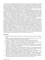
Figure 17.12 depicts EI as a function of the angle δ, pretension of the top string, and the rigidity
ratio K which is deﬁned as the ratio of the axial rigidity of the strings to the axial rigidity of the
bars, i.e., K = (EA)
s
/(EA)
b
. The pretension is measured as a function of the prestrain in the top
string Σ
0
. In obtaining Figure 17.12, the bars were assumed to be equal in diameter and the strings
were also assumed to be of equal diameter. Both the bars as well as the strings were assumed to
be made of steel for which Young’s modulus of elasticity E was taken to be 2.06 × 10
11
N/m
2
, and

the yield strength of the steel σ
y
was taken to be 6.90 × 10
8
N/m
2
. In Figure 17.12, EI is plotted
against the ratio of the external load F to the yield force of the string. The yield force of the string
is deﬁned as the force that causes the strings to reach the elastic limit. The yield force for the
strings is computed as
Yield force of string = σ
y
A
s
,
where σ
y
is the yield strength and A
s
is the cross-sectional area of the string. The external force F
was gradually increased until at least one of the strings yielded.
The following conclusions can be drawn from Figure 17.12:
1. Figure 17.12(a) suggests that the bending rigidity EI of a tensegrity unit with all taut strings
increases with an increase in the angle δ, up to a maximum at δ = 90°.
2. Maximum bending rigidity EI is obtained when none of the strings is slack, and the EI is
approximately constant for any external force until one of the strings go slack.

At 0 t t t t
00
== ≥, [ ], .

0
00
-

0
0
T
bars
strings strings
8596Ch17Frame Page 327 Friday, November 9, 2001 6:33 PM
© 2002 by CRC Press LLC
3. Figure 17.12(b) shows that the pretension does not have much effect on the magnitude of
EI of a planar tensegrity unit. However, pretension does play a remarkable role in preventing
the string from going slack which, in turn, increases the range of the constant EI against
external loading. This provides robustness of EI predictions against uncertain external forces.
This feature provides robustness against uncertainties in external forces.
4. In Figure 17.12(c) we chose structures having the same geometry and the same total stiffness,
but different K, where K is the ratio of the axial rigidity of the bars to the axial rigidity of
the strings. We then see that K has little inﬂuence on EI as long as none of the strings are
slack. However, the bending rigidity of the tensegrity unit with slack string inﬂuenced K,
with maximum EI occurring at K = 0 (rigid bars).
It was also observed that as the angle δ is increased or as the stiffness of the bar is decreased,
the force-sharing mechanism of the members of the tensegrity unit changes quite noticeably. This
phenomena is seen only in the case when the top string is slack. For example, for K = 1/9 and ε
0
=
0.05%, for small values of δ, the major portion of the external force is carried by the bottom string,
whereas after some value of δ (greater than 45°), the major portion of the external force is carried
by the vertical side strings rather than the bottom string. In such cases, the vertical side strings
FIGURE 17.12 Bending rigidity EI of the planar tensegrity unit for (a) different initial angle δ with rigidity ratio

K = 1/9 and prestrain in the top string ε
0
= 0.05%, (b) different ε
0
with K = 1/9, (c) different K with δ = 60° and ε
0
=
0.05%. L
bar
for all cases is 0.25 m.
(a) (b) (c)
8596Ch17Frame Page 328 Friday, November 9, 2001 6:33 PM
© 2002 by CRC Press LLC
could reach their elastic limit prior to the bottom string. Similar phenomena were also observed
for a case of K = 100, δ = 60°, and ε
0
= 0.05%. In such cases, as shown in Figure 17.12(a) for δ =
70° and δ = 75°, the EI drops drastically once the top string goes slack. Figure 17.13 summarizes
the conclusions on bending rigidity, where the arrows indicate increasing directions of δ, t
0
, or K.
Note that when t
0
is the pretension applied to the top string, the pretension in the vertical side
strings is equal to t
0
/tan δ. The cases of δ > 80° were not computed, but it is clear that the bending
rigidity is a step function as δ approaches 90°, with EI constant until the top string becomes slack,
then the EI goes to zero as the external load increases further.
17.2.1.2 Bending Rigidity of the Planar Tensegrity for the Rigid Bar Case (K = 0)

The previous section brieﬂy described the basis of the calculations for Figure 17.11. The following
sections consider the special case K = 0 to show more analytical insight. The nonslack case describes
the structure when all strings exert force. The slack case describes the structure when string 3 exerts
zero force, due to the deformation of the structure. Therefore, the force in string 3 must be computed
to determine when to switch between the slack and nonslack equations.
17.2.1.2.1 Some Relations from Geometry and Statics
Nonslack Case: Summing forces at each node we obtain the equilibrium conditions
ƒ
c
cos δ = F + t
3
– t
2
sin θ (17.6)
ƒ
c
cos δ = t
1
+ t
2
sin θ – F (17.7)
ƒ
c
sin δ = t
2
cos θ, (17.8)
where ƒ
c
is the compressive load in a bar, F is the external load applied to the structure, and t
i

is
the force exerted by string i deﬁned as
t
i
= k
i
(l
i
– l
i0
). (17.9)
The following relations are deﬁned from the geometry of Figure 17.11:
l
1
= L
bar
cos δ + L
bar
tan θ sin δ
l
2
= L
bar
sin δ sec θ
l
3
= L
bar
cos δ – L
bar

sin δ tan θ
h = L
bar
sin δ, (17.10)
FIGURE 17.13 Trends relating geometry δ, prestress t
0
, and material K.
8596Ch17Frame Page 329 Friday, November 9, 2001 6:33 PM
© 2002 by CRC Press LLC
where l
i
denote the geometric length of the strings. We will ﬁnd the relation between δ and θ by
eliminating f
c
and F from (17.6)–(17.8)
(17.11)
Substitution of relations (17.10) and (17.9) into (17.11) yields
(17.12)
If k
i
= k, then (17.12) simpliﬁes to
(17.13)
Slack Case: In order to ﬁnd a relation between δ and θ for the slack case when t
3
has zero
tension, we use (17.12) and set k
3
to zero. With the simpliﬁcation that we use the same material
properties, we obtain
0 = L

bar
tan θ sin δ tan δ + 2l
20
cos θ – l
10
tan δ – L
bar
sin δ. (17.14)
This relationship between δ and θ will be used in (17.22) to describe bending rigidity.
17.2.1.2.2 Bending Rigidity Equations
The bending rigidity is deﬁned in (17.3) in terms of ρ and F. Now we will solve the geometric and
static equations for ρ and F in terms of the parameters θ, δ of the structure. For the nonslack case,
we will use (17.13) to get an analytical formula for the EI. For the slack case, we do not have an
analytical formula. Hence, this must be done numerically.
From geometry, we can obtain ρ,
Solving for ρ we obtain
(17.15)
Nonslack Case: In the nonslack case, we now apply the relation in (17.13) to simplify (17.15)
(17.16)
cos tan .θδ=
+tt
t
13
2
2
cos
( cos tan sin ) ( cos tan sin )
( sin sec )
tan
+

.θ
δθδ δθδ
δθ
δ=
−+ − −
−
kL L l kL L l
kL l
bar bar bar bar
bar
110330
220
2
tan δθβθ=
+
2
20
10 30
l
ll
cos = cos .
tan
()
θ
ρ
=
+
l
h
1

2
2
.
ρ
θ
δθδ
θ
δ
δ
θ
=−
+
−
=
l
h
LL L
L
bar bar bar
bar
1
22
22
2
tan
cos tan sin
tan
sin
cos
tan

.

=

ρ
θβ θ
=
+
L
bar
2
1
1
22
tan cos
.
8596Ch17Frame Page 330 Friday, November 9, 2001 6:33 PM
© 2002 by CRC Press LLC
From (17.6)–(17.8) we can solve for the equilibrium external F
– k
3
L
bar
cos δ + k
3
L
bar
sin δ tan θ + k
3
l

30
). (17.17)
Again, using (17.13) and k
i
= k, Equation (17.17) simpliﬁes to
(17.18)
We can substitute (17.18) and (17.16) into (17.3)
(17.19)
and we obtain the bending rigidity of the planar structure with no slack strings present. The
expression for string length l
3
in the nonslack case reduces to
(17.20)
This expression can be used to determine the angle which causes l
3
to become slack.
Slack Case: Similarly, for the case when string 3 goes slack, we set k
3
= 0 and k
i
= k in (17.17),
which yield simply
(17.21)
and
(17.22)
See Figure 17.12(c) for a plot of EI for the K = 0 (rigid bar) case.
17.2.1.2.3 Constants and Conversions
All plots shown are generated with the following data which can then be converted as follows if
necessary.
Ftt t

kL kL kl
kL kl
bar bar
bar
=+ −
=+ −
+−
1
2
2
1
2
22
12 3
11 110
2220
( sin )
( cos tan sin
sin tan sin
θ
δθδ
δθ θ
F
kL
k
ll l
bar
=
+
−−

2
1
2
2
22
10 30 20
βθ
βθ
θ
sin
cos
sin ( + ).

El
LkL
k
ll l
bar bar
=
+
+
−−






22
22

22
10 30 20
21
2
1
2
2
βθ
βθθ
βθ
βθ
θ
cos
( cos ) (sin )
sin
cos
sin , ( + )

lL
bar
3
22
=
1 + cos
1−β θ
βθ

sin
.

Ftt
kL kL kl kl
slack
bar bar
= ( + )
= (
1
2
2
1
2
32
12
10 20
sin
cos tan sin sin )
θ
δθδ θ+−−
EI
L
kL kL kl kl
slack
bar
bar bar
=

(
2
10 20
4

32
sin cos
tan
cos tan sin sin ).
δδ
θ
δθδ θ+−−
8596Ch17Frame Page 331 Friday, November 9, 2001 6:33 PM
© 2002 by CRC Press LLC
Young’s Modulus, E = 2.06 × 10
11
N/m
2
Yield Stress, σ = 6.9 × 10
8
N/m
2
Diameter of Tendons = 1 mm
Cross-Sectional Area of Tendon = 7.8540 × 10
–7
m
2
Length of Bar, L
bar
= .25 m
Prestress = e
0
Initial Angle = δ
0
The spring constant of a string is

(17.23)
The following equation can be used to compute the equivalent rest length given some measure
of prestress t
0
t
0
= (EA)
s
e
0
= k(l – l
0
)
. (17.24)
17.2.1.3 Effective Bending Rigidity with Slack String (K > 0)
As noted earlier, the tensegrity unit is a statically indeterminate structure (meaning that matrix A
is not full column rank) as long as the strings remain taut during the application of the external
load. However, as soon as one of the strings goes slack, the tensegrity unit becomes statically
determinate. In the following, an expression for bending rigidity of the tensegrity unit with an
initially slack top string is derived. Even in the case of a statically determinate tensegrity unit with
slack string, the problem is still a large displacement and nonlinear problem. However, a linear
solution, valid for small displacements only, resulting in a quite simple and analytical form can be
found. Based on the assumptions of small displacements, an analytical expression for EI of the
tensegrity unit with slack top string has been derived in Appendix 17.B and is given below.
(17.25)
The EI obtained from nonlinear analysis, i.e., from (17.3) together with (17.5), is compared with
the EI obtained from linear analysis, i.e., from (17.25), and is shown in Figure 17.14. Figure 17.14
shows that the linear analysis provides a lower bound to the actual bending rigidity. The linear
estimation of EI, i.e., (17.25), is plotted in Figure 17.15 as a function of the initial angle δ for
different values of the stiffness ratio K. Both bars and the strings are assumed to be made of steel,

as before. It is seen in Figure 17.15 that the EI of the tensegrity unit with slack top string attains
a maximum value for some value of δ. The decrease of EI (after the maximum) is due to the change
in the force sharing mechanism of the members of the tensegrity unit, as discussed earlier. For
small values of δ, the major portion of the external force is carried by the bottom string, whereas
for larger values of δ, the vertical side strings start to share the external force. As δ is further

k
EA
L
bar
=
cos( )
.
δ
0
lL
EAe
k
bar
00
0
=
cos( )δ−
EI
LEA
K
bar
s
≈
++

1
22
2
23
33
( ) sin cos
(sin cos )
.
δδ
δδ
8596Ch17Frame Page 332 Friday, November 9, 2001 6:33 PM
© 2002 by CRC Press LLC
increased, the major portion of the external force is carried by the vertical side strings rather than
the bottom string. This explains the decrease in EI with the increase in δ after some values of δ
for which EI is maximum.
The locus of the maximum EI is also shown in Figure 17.15. The maximum value of EI and the
δ for which EI is maximum depend on the relative stiffness of the string and the bars, i.e., they
depend on K. From Figure 17.15 note that the maximum EI is obtained when the bars are much
FIGURE 17.14 Comparison of EI from nonlinear analysis with the EI from linear analysis with slack top string
(L
bar
= 0.25 m, δ = 60° and K = 1/9).
FIGURE 17.15 EI with slack top string with respect to the angle δ for L
bar
= 0.25m.
8596Ch17Frame Page 333 Friday, November 9, 2001 6:33 PM
© 2002 by CRC Press LLC
stiffer than the strings. EI is maximum when the bars are perfectly rigid, i.e., K → 0. It is seen in
Figure 17.15 and can also be shown analytically from (17.25) that for the case of bars much stiffer
than the strings, K → 0, the maximum EI of the tensegrity unit with slack top string is obtained

when δ = 45°. In constrast, note from Figure 17.12(a) that when no strings are slack, the maximum
bending rigidity occurs with δ = 90°.
17.2.2 Mass Efﬁciency of the C2T4 Class 1 Tensegrity in Bending
This section demonstrates that beams composed of tensegrity units can be more efﬁcient than
continua beams. We make this point with a very speciﬁc example of a single-unit C2T4 structure.
In a later section we allow the number of unit cells to approach inﬁnity to describe a long beam.
Let Figure 17.16 describe the conﬁguration of interest. Note that the top string is slack (because
the analysis is easier), even though the stiffness will be greater before the string is slack. The
compressive load in the bar, F
c
.
F
c
= F/cos δ
Designing the bar to buckle at this force yields
where the mass of the two bars is (ρ
1
= bar mass density)
Hence, eliminating r
bar
gives for the force
The moment applied to the unit is
(17.30)
To compare this structure with a simple classical structure, suppose the same moment is applied
to a single bar of a rectangular cross section with b units high and a units wide and yield strength
σ
y
such that
(17.31)
FIGURE 17.16 C2T4 tensegrity with slack top string.

F
Er
L
Lr
c
bar
bar
bar bar
=
π
3
1
4
2
4

( = length, radius of bar,,) .
mm Lrr
m
L
b bar bar bar
b
bar
== ⇒= 22
2
11
22
1
πρ
πρ

.

F
E
L
m
L
E
L
m
c
bar
b
bar bar
b
=






=






π

πρ
π
ρ
3
1
2
2
2
1
22
1
1
24
2
44 16

MFL
E
L
m
bar
bar
b
==sin cos sin .δ
π
ρ
δδ
1
1
23

2
16

M
I
IabC
b
mLab
y
== ==
σ
ρ
C
,,, ,
1
12 2
3
0
00

8596Ch17Frame Page 334 Friday, November 9, 2001 6:33 PM
© 2002 by CRC Press LLC
then, for the rectangular bar
(17.32)
Equating (17.30) and (17.32), using L
0
= L
bar
cos δ, yields the material/geometry conservation
law ( is a material property and g is a property of the geometry)

(17.33)
The mass ratio µ is inﬁnity if δ = 0°, 90°, and the lower bound on the mass ratio is achieved
when = 26.565°.
Lemma 17.1 Let σ
y
denote the yield stress of a bar with modulus of elasticity E
1
and dimension
a × b × L
0
. Let M denote the bending moment about an axis perpendicular to the b dimension. M
is the moment at which the bar fails in bending. Then, the C2T4 tensegrity fails at the same M but
has less mass if and minimal mass is achieved at .
Proof: From (17.33),
(17.34)
where the lower bound is achieved at by setting ∂g/∂δ = 0 and solving
cos
2
δ = 4sin
2
δ, or tan δ = 1/2. ❏
For steel with (σ
y
, E
1
) = (6.9 × 10
8
, 2 × 10
11
)

(17.35)
where the lower bound is achieved for = 26.565°. Hence, for geometry of the steel
comparison bar given by then m
b
= 0.51 m
0
, showing
49% improvement in mass for a given yield moment. For the geometry
, m
b
= 0.2m
0
, showing 80% improvement in mass for a given yield
moment, M. The main point here is that strength and mass efﬁciency are achieved by geometry
(δ = 26.565°), not materials.
It can be shown that the compressive force in a bar when the system C2T4 is under a pure
bending load exhibits a similar robustness property that was shown with the bending rigidity. The
force in a bar is constant until a string becomes slack, which is shown in Figure 17.17.
17.2.3 Global Bending of a Beam Made from C2T4 Units
The question naturally arises “what is the bending rigidity of a beam made from many tensegrity
cells?” 17.2.3.2 answers that question. First, in Section 17.2.3.1 we review the standard beam theory.
17.2.3.1 Bucklings Load
For a beam loaded as shown in Figure 17.18, we have
(17.36)

M
m
aL
y
=

σ
ρ
0
2
0
2
0
2
6
.
σ

µ
δ
π
σσ
σ
δδ
2

0
=






===
∆∆∆

m
m
g
E
g
L
a
b
y
2
1
0
4
3
,,
cos sin
δ=
−
tan ( )
1
12
σ
g < (),3πδ
δ=
−
tan ( )
1
12
µ
δ

π
σ
δ
π
σ
2
0
33
3 493856=≥ =ggg
L
a
,,.
()δπσ3 g δ=
−
tan ( )
1
12
(),Nm
2

µ
δ
π
σ
2

=≥
3
0 008035869
0

g
L
a
.
tan ( )
−1
12
La
o
0
1
50 1 2 26 565== =
{}
−
, tan ( ) . ,and δ

La
0
o
==
{}
20 26 565and δ .

EI
dv
dz
Fv Fe
2
2

=− −
8596Ch17Frame Page 335 Friday, November 9, 2001 6:33 PM
© 2002 by CRC Press LLC
equivalently,
(17.37)
where
p
2
= F/EI, (17.38)
where EI is the bending rigidity of the beam, v is the transverse displacement measured from the
neutral axis (denoted by the dotted line in Figure 17.18), z represents the longitudinal axis, L is
FIGURE 17.17 Comparison of force in the bar obtained from linear and nonlinear analysis for pure bending
loading. (Strings and bars are made of steel, Young’s modulus E = 2.06 × 10
11
N/m
2
, yield stress σ
y
= 6.90 × 10
8
N/m
2
, diameter of string = 1 mm, diameter of bar = 3 mm, K = 1/9, δ = 30°, ε
0
= 0.05% and L
0
= 1.0 m.)
FIGURE 17.18 Bending of a beam with eccentric load at the ends.

dv

dz
pv pe
2
2
22

+=−
8596Ch17Frame Page 336 Friday, November 9, 2001 6:33 PM
© 2002 by CRC Press LLC
the length of the beam, e is the eccentricity of the external load F. The eccentricity of the external
load is deﬁned as the distance between the point of action of the force and the neutral axis of the
beam.
The solution of the above equation is
v = A sin pz + B cos pz – e (17.39)
where constants A and B depend on the boundary conditions. For a pin–pin boundary condition,
A and B are evaluated to be
, and B = e (17.40)
Therefore, the deﬂection is given by
(17.41)
17.2.3.2 Buckling of Beam with Many C2T4 Tensegrity Cells
Assume that the beam as shown in Figure 17.18 is made of n small tensegrity units similar to the
one shown in Figure 17.11, such that L = nL
0
, and the bending rigidity EI appearing in (17.36) and
(17.38) is replaced by EI given by (17.25). Also, since we are analyzing a case when the beam
breaks, we shall assume that the applied force is large compared to the pretension. The beam
buckles at the unit receiving the greatest moment. Because the moment varies linearly with the
bending and the bending is greatest at the center of the beam, the tensegrity unit at the center
buckles. The maximum moment M
max

leading to the worst case scenario is related to the maximum
deﬂection at the center v
max
. From (17.41),
. (17.42)
Simple algebra converts this to
(17.43)
The worst case M
max
is equal to Fv
max
+ Fe and is given by
(17.44)
Now we combine this with the buckling formula for one tensegrity unit to get its breaking moment
(17.45)
Ae
pL
= tan
2
ve
pL
pz pz=+−






tan sin cos
2

1
ve
pL pL pL
max
tan sin cos=+−






22 2
1
ve
pL
max
cos
=
−










1

2
1
M
F
nL
F
EI
e
max
cos
=






0
2
MeFe
EI
L
break
B
b
==
()
π
δ
2

0
2
3
cos
8596Ch17Frame Page 337 Friday, November 9, 2001 6:33 PM
© 2002 by CRC Press LLC
Thus, from Equations (17.44) and (17.45), if F exceeds F
gB
given by
(17.46)
the central unit buckles, and F
gB
is called the global buckling load.
Multiplying both sides of (17.46) by (nL
0
)
2
and introducing three new variables,
F = F
gB
(nL
0
)
2
, (17.47)
we rewrite (17.46) as
(17.48)
Equivalently,
, (17.49)
where η is a function deﬁned as

. (17.50)
η is a monotonically increasing function in
, (17.51)
satisfying
η ≥ F (17.52)
It is interesting to know the buckling properties of the beam as the number of the tensegrity
elements become large. As n → ∞, (nL
0
)
2
→ ∞, and from (17.49) and (17.51)
(17.53)
and Ᏺ approaches the limit from below. From Equations (17.47) and (17.49),
(17.54)
Thus, for large n, using (17.53), we get
F
EI
L
gB
nL
F
EI
b
gB
cos
()
cos

0
2

2
0
2
3




=
π
δ

P =
()
π
δ
2
0
2
3
EI
L
b
cos ,

K =
1
2
1
EI

,
F
KF
P
cos
()
= nL
2
0
2
η()FP= nL
2
0
2

η()
cos ( )
F
F
KF
=

0
2
1
2
2
≤≤





F
K
π

FP
K
=
[]
→




−
η
π
12
0
2
2
2
2
2
nL
F
nL
nL

gB
=
()
[]
−
11
2
0
2
12
0
2
η P
8596Ch17Frame Page 338 Friday, November 9, 2001 6:33 PM
© 2002 by CRC Press LLC
(17.55)
The global buckling load as given by (17.55) is exactly the same as the classical Euler’s buckling
equation evaluated for the bending rigidity EI of the tensegrity unit. Therefore, asymptotically the
buckling performance of the beam depends only on the characteristics of EI and just as a classical
beam.
Note, for each n
The implication here is that the standard Euler buckling formula applies where EI is a function
of the geometrical properties of the tensegrity unit. Figure 17.12(a) shows that EI can be assigned
any ﬁnite value. Hence, the beam can be arbitrarily stiff if the tensegrity unit has horizontal length
arbitrarily small. This is achieved by using an arbitrarily large number of tensegrity units with large
δ (arbitrarily close to 90°). More work is needed to deﬁne practical limits on stiffness.
17.2.4 A Class 1 C2T4 Planar Tensegrity in Compression
In this section we derive equations that describe the stiffness of the Class 1 C2T4 planar tensegrity
under compressive loads. The nonslack case describes the structure when all strings exert force.
The slack case describes the structure when string 3 and string 1 exert zero force, due to the

deformation of the structure. Therefore, the force in string 3 and string 1 must be computed in
order to determine when to switch between the slack and nonslack equations. We make the
assumption that bars are rigid, that is, K = 0.
17.2.4.1 Compressive Stiffness Derivation
Nonslack Case: Summing forces at each node we obtain the equilibrium conditions
(17.56)
(17.57)
, (17.58)
where f
c
is the compressive load in a bar, F is the external load applied to the structure, and t
i
is
the force exerted by string i deﬁned as
.
The following relations are deﬁned from the geometry of Figure 17.19:

F
nL
nL
n
EI
L
gB
EI
≈





≈




≈
11
2
1
11
2
1
1
2
0
2
2
2
2
0
2
2
1
4
1
2
2
0
2
π

π
π
K

L
0
2
F
n
EI
L
gB
≤
1
2
2
0
2
π
.
fFt
c
cos δ= +
3
fFt
c
cos δ= +
1
ft

c
sin δ=
2
tkll
iiii
=−
()
0
8596Ch17Frame Page 339 Friday, November 9, 2001 6:33 PM
© 2002 by CRC Press LLC
(17.59)
Solving for F we obtain
(17.60)
Using the relation L
0
= L
bar
cos δ and tan results in
(17.61)
We will also make the assumption now that all strings have the same material properties,
speciﬁcally, l
i0
= l
0
. Now, the stiffness can be computed as
(17.62)
Similarly, for the slack case, when t
1
and t
3

are slack, we follow the same derivation setting t
1
=
t
3
= 0 in (17.56)–(17.58)
. (17.63)
Substitution of L
0
= L
bar
cos δ yields
. (17.64)
Taking the derivative with respect to L
0
gives
FIGURE 17.19 C2T4 in compression.
lL
bar
1
= cosδ
lL
bar
2
= sin δ
lL
bar
3
= cosδ
Fkl

l
=−(
tan
).
10
20
δ
δ=
−LL
L
bar
2
0
2
0
Fkl
kl L
LL
bar
=−
−
10
20 0
2
0
2
K
dF
dL
kl

LL
kl L
LL
kl L
LL
bar
bar
bar
bar
=− =
−
+
−
()
=
−
()
∆
0
0
2
0
2
00
2
2
0
2
0
2

2
0
2
3
2
3
2
.
FkL
kl
slack bar
=−cos
tan
δ
δ
0
FkL
kl L
LL
slack
bar
=−
−
0
00
2
0
2
8596Ch17Frame Page 340 Friday, November 9, 2001 6:33 PM
© 2002 by CRC Press LLC

. (17.65)
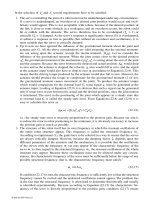
A plot of stiffness for the nonslack and slack case vs. applied force is given in Figure 17.20,
where k = 9.1523 × 10
5
N/m, δ = 45º, L
bar
= 0.25 m, and the force, F, ranges between 0 and 600 N.
17.2.5 Summary
Tensegrity structures have geometric structure that can be designed to achieve desirable mechanical
properties. First, this chapter demonstrates how bending rigidity varies with the geometrical param-
eters. The bending rigidity is reduced when a string goes slack, and pretension delays the onset of
slack strings. The important conclusions made in this section are
• Beams made from tensegrity units can be stiffer than their continuous beam counterparts.
• Pretension can be used to maintain a constant bending rigidity over a wider range of external
loads. This can be important to robustness, when the range of external loads can be uncertain.
• For larger loads the bending stiffness is dominated by geometry, not pretension. This explains
the mass efﬁciency of tensegrity structures since one can achieve high stiffness by choosing
the right geometry.
• The ratio of mass to bending rigidity of the C2T4 tensegrity is shown to be smaller than for
a rectangular cross-section bar, provided the geometry is chosen properly (angle between
bars must be less than 53°). Comparisons to a conventional truss would be instructive. There
are many possibilities.
17.3 Planar Class K Tensegrity Structures Efﬁcient
in Compression
It is not hard to show that the Class 1 C2T4 tensegrity of Figure 17.19 is not as mass efﬁcient as
a single rigid bar. That is, the mass of the structure in Figure 17.19 is greater than the mass of a
FIGURE 17.20 Stiffness of C2T4 vs. applied load, plotted until strings yield.
0 100 200 300 400 500 600
0.8
1

1.2
1.4
1.6
1.8
2
x 10
6
Applied Force
Stiffness
Compression
K
dF
dL
k
kl
LL
kl L
LL
slack
slack
bar
bar
=− =− +
−
+
−
()
0
0
2

0
2
00
2
2
0
2
3
2
=
−
()
−








k
lL
LL
bar
bar
0
2
2
0

2
3
2
1
8596Ch17Frame Page 341 Friday, November 9, 2001 6:33 PM
© 2002 by CRC Press LLC
single bar which buckles at the same load 2F. This motivates the examination of Class 2 tensegrity
structures which have the potential of greater strength and stiffness due to ball joints that can
efﬁciently transfer loads from one bar to another. Compressive members are disconnected in the
traditional deﬁnition
2
of tensegrity structures, which we call Class 1 tensegrity. However, if stiff
tendons connecting two nodes are very short, then for all practical purposes, the nodes behave as
though they are connected. Hence, Class 1 tensegrity generates Class k tensegrity structures as
special cases when certain tendons become relatively short. Class k tensegrity describes a network
of axially loaded members in which the ends of not more than k compressive members are connected
(by ball joints, of course, because torques are not permitted) at nodes of the network.
In this section, we examine one basic structure that is efﬁcient under compressive loads. In order
to design a structure that can carry a compressive load with small mass we employ Class k tensegrity
together with the concept of self-similarity. Self-similar structures involve replacing a compressive
member with a more efﬁcient compressive system. This algorithm, or fractal, can be repeated for
each member in the structure. The basic principle responsible for the compression efﬁciency of
this structure is geometrical advantage, combined with the use of tensile members that have been
shown to exhibit large load to mass ratios. We begin the derivation by starting with a single bar
and its Euler buckling conditions. Then this bar is replaced by four smaller bars and one tensile
member. This process can be generalized and the formulae are given in the following sections. The
objective is to characterize the mass of the structure in terms of strength and stiffness. This allows
one to design for minimal mass while bounding stiffness. In designing this structure there are trade-
offs; for example, geometrical complexity poses manufacturing difﬁculties.
The materials of the bars and strings used for all calculations in this section are steel, which has

the mass density ρ = 7.862 , Young’s modulus E = 2.06
11
and yield strength σ = 6.9
8
. Except when speciﬁed, we will normalize the length of the structures L
0
= 1 in numerical
calculations.
17.3.1 Compressive Properties of the C4T2 Class 2 Tensegrity
Suppose a bar of radius r
0
and length L
0
, as shown in Figure 17.21 buckles at load F. Then,
, (17.66)
where E
0
is the Young’s modulus of the bar material.
The mass of the bar is
, (17.67)
where ρ
0
is the mass density of the bar.
Equations (17.66) and (17.67) yield the force–mass relationship
. (17.68)
FIGURE 17.21 A bar under compression.
gcm
3
Nm
2

Nm
2
F
Er
L
=
0
3
0
4
0
2
π
mrL
000
2
0
=ρ π
F
Em
L
=
00
2
0
2
0
4
4
π

ρ
8596Ch17Frame Page 342 Friday, November 9, 2001 6:33 PM
© 2002 by CRC Press LLC
Now consider the four-bar pinned conﬁguration in Figure 17.22, which is designed to buckle at
the same load F. Notice that the Class 2 tensegrity of Figure 17.22 is in the dual (where bars are
replaced by strings and vice versa) of the Class 1 tensegrity of Figure 17.3(b), and is of the same
type as the Class 2 tensegrity in Figure 17.3(c).
We ﬁrst examine the case when tendon t
h
is slack. The four identical bars buckle at the bar
compressive load F
1
and the mass of each of the four bars is Hence,
(17.69)
where (r
1
, L
1
, E
1
, ρ
1
) is respectively, the radius, length, Young’s modulus, and mass density of each
bar, and the mass of the system C4T1 in Figure 17.22 is
Since from the Figure 17.22, the length of each bar is L
1
and the compressive load in each bar is
F
1
given by,

, (17.70)
then, from (17.68)–(17.70)
. (17.71)
Note from (17.70) that the C4T2 structure with no external force F and tension t
h
= F
x
in the
horizontal string, places every member of the structure under the same load as a C4T1 structure
(which has no horizontal string) with an external load F = F
x
. In both cases, .
Solving for the mass ratio, from (17.71)
(17.72)
For slack tendon t
h
= 0, note that µ
1
< 1 if δ < cos
–1
= 29.477°. Of course, in the slack case
(when t
h
= 0), one might refer to Figure 17.22 as a C4T1 structure, and we will use this designation
to describe the system of Figure 17.22 when t
h
is slack. Increasing pretension in t
h
to generate the
nonslack case can be examined later. The results are summarized as follows:

FIGURE 17.22 A C4T2 planar Class 2 tensegrity structure.
14
1
m .
F
Er
L
mrLF
Em
L
1
1
2
1
4
1
2
111
2
11
11
2
1
2
1
4
4
4
64
== =

π
ρπ
π
ρ
,,,
mrL
111
2
1
4=ρπ .
L
L
F
Ft
h
1
0
1
22
==
+
cos
,
cosδδ

F
Em
L
Ft
h

1
11
2
1
2
1
4
64 2
==
+
π
ρδcos
FF
x1
2= cosδ
µ
ρ
ρδ
1
1
0
1
0
0
1
5
1
2
1
2

=






=
+










∆
m
m
E
E
t
F
h
cos
1
2

1
5
()
8596Ch17Frame Page 343 Friday, November 9, 2001 6:33 PM
© 2002 by CRC Press LLC
Proposition 17.1 With slack horizontal string t
h
= 0, assume that strings are massless, and that
the C4T1 system in Figure 17.22 is designed to buckle at the same load F as the original bar of
mass m
0
in Figure 17.21. Then, the total mass m
1
of the C4T1 system is , which
is less than m
0
whenever δ < 29.477 degrees.
Proof: This follows by setting µ
1
= 1 in (17.72).
Some illustrative data that reﬂect the geometrical properties of the C4T1 in comparison with a
bar which buckles with the same force F are shown in Table 17.1. For example, when δ = 10
°
, the
C4T1 requires only 73.5% of the mass of the bar to resist the same compressive force. The data
in Table 17.1 are computed from the following relationships for the C4T1 structure. The radius of
each bar in the C4T1 system is r
1
,
and

From this point forward we will assume the same material for all bars. Hence,
Likewise,
and
Also,
TABLE 17.1 Properties of the C4T1 Structure
a
δ = 10° δ = 20°
r
1
.602r
0
.623r
0
m
1
.735m
0
.826m
0
L
1
.508L
0
.532L
0
a
Strings are assumed massless.
mm
10
5

2
1
2
=
−
( cos )δ
L
r
1
1
.844
0
0
L
r
.854
0
0
L
r
r
m
L
1
2
1
11
4
=
ρπ

r
m
L
0
2
0
00
=
ρπ
.
r
r
1
0
4
3
1
8






=
cos
.
δ
L
L

1
0
1
2






=
cos
,
δ
r
r
L
L
1
0
4
1
0
3







=






.
L
r
L
r
L
r
1
1
0
3
0
0
0
8
2
1
2
1
4
1
4
=

()
=




cos
cos cos
.
δ
δδ
8596Ch17Frame Page 344 Friday, November 9, 2001 6:33 PM
© 2002 by CRC Press LLC
17.3.2 C4T2 Planar Tensegrity in Compression
In this section we derive equations that describe the stiffness of the C4T2 planar tensegrity under
compressive loads. Pretension would serve to increase the restoring force in the string, allowing
greater loads to be applied with smaller deformations. This is clearly shown in the force balance
Equation (17.70), where pretension can be applied through the use of the rest length L
h0
of the
string, and t
h
= k
h
(L
0
– L
h0
), where k
h

is the stiffness of the horizontal string.
17.3.2.1 Compressive Stiffness Derivation
From Figure 17.22, the equilibrium conﬁguration can be expressed as
, (17.73)
where t, L
0
, L
t
, and L
t0
are the tension, length of the structure, length of the string, and the rest
length of the vertical string, respectively. The length of the string can be written as
,
where L
1
denotes the length of one bar. This relation simpliﬁes the force balance equation to
. (17.74)
Figure 17.23 shows the plot of the load deﬂection curve of a C4T2 structure with different δ.
The compressive stiffness can be calculated by taking the derivative of (17.74) with respect to L
0
as follows,
(17.75)
FIGURE 17.23 Load-deﬂection curve of C4T2 structure with different δ (K
e
= 1, K
h
= 3K
t
= 3, L
l