Electrical Engineering Mechanical Systems Design Handbook Dorf CRC Press 2002819s_10 pdf

(17.123)
where r and L are the cross-section radius and length of bars or strings when the C4T1
i
structure
is under external load F.
17.3.5.1 C4T1
1
at δ = 0°
At δ = 0°, it is known from the previous section that the use of mass is minimum while the stiffness
is maximum. Therefore, a simple analysis of C4T1
1
at δ = 0 will give an idea of whether it is
possible to reduce the mass while preserving stiffness.
For the C4T1
0
structure, the stiffness is given by
(17.124)
For a C4T1
1
structure at δ = 0°, i.e., two pairs of parallel bars in series with each other, the length
of each bar is L
0
/2 and its stiffness is
(17.125)
For this four-bar arrangement, the equivalent stiffness is same as the stiffness of each bar, i.e.,
(17.126)
To preserve stiffness, it is required that
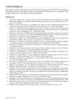
FIGURE 17.41 Stiffness-to-mass ratio vs. δ for l
0
= 30.
K

m
i
i
k
Er
L
=
π
2
,
K
Er
L
0
0
2
0
=
π
.
k
Er
L
Er
L
b
==
ππ
1
2

1
1
2
0
2
.
K
Er
L
1
1
2
0
2
=
π
.
KK
Er
L
Er
L
10
1
2
0
0
2
0
2

=
=
π
π
.
8596Ch17Frame Page 362 Friday, November 9, 2001 6:33 PM
© 2002 by CRC Press LLC
So,
(17.127)
Then, the mass of C4T1
1
at δ = 0° for stiffness preserving design is
(17.128)
which indicates, at δ = 0°, that the mass of C4T1
1
is equal to that of C4T1
0
in a stiffness-preserving
design. Therefore, the mass reduction of C4T1
i
structure in a stiffness-preserving design is unlikely
to happen. However, if the horizontal string t
h
is added in the C4T1
1
element to make it a C4T2
element, then stiffness can be improved, as shown in (17.76).
17.3.6 Summary
The concept of self-similar tensegrity structures of Class k has been illustrated. For the example of
massless strings and rigid bars replacing a bar with a Class 2 tensegrity structure C4T1 with specially

chosen geometry, δ < 29°, the mass of the new system is less than the mass of the bar, the strength of
the bar is matched, and a stiffness bound can be satisfied. Continuing this process for a finite member
of iterations yields a system mass that is minimal for these stated constraints. This optimization problem
is analytically solved and does not require complex numerical codes. For elastic bars, analytical
expressions are derived for the stiffness, and choosing the parameters to achieve a specified stiffness
is straightforward numerical work. The stiffness and stiffness-to-mass ratio always decrease with self-
similar iteration, and with increasing angle δ, improved with the number of self-similar iterations,
whereas the stiffness always decreases.
17.4 Statics of a 3-Bar Tensegrity
17.4.1 Classes of Tensegrity
The tensegrity unit studied here is the simplest three-dimensional tensegrity unit which is comprised
of three bars held together in space by strings to form a tensegrity unit. A tensegrity unit comprising
three bars will be called a 3-bar tensegrity. A 3-bar tensegrity is constructed by using three bars in
each stage which are twisted either in clockwise or in counter-clockwise direction. The top strings
connecting the top of each bar support the next stage in which the bars are twisted in a direction
opposite to the bars in the previous stage. In this way any number of stages can be constructed
which will have an alternating clockwise and counter-clockwise rotation of the bars in each
successive stage. This is the type of structure in Snelson’s Needle Tower, Figure 17.1. The strings
that support the next stage are known as the “saddle strings (S).” The strings that connect the top
of bars of one stage to the top of bars of the adjacent stages or the bottom of bars of one stage to
the bottom of bars of the adjacent stages are known as the “diagonal strings (D),” whereas the
strings that connect the top of the bars of one stage to the bottom of the bars of the same stage are
known as the “vertical strings (V).”
Figure 17.42 illustrates an unfolded tensegrity architecture where the dotted lines denote the
vertical strings in Figure 17.43 and thick lines denote bars. Closure of the structure by joining
points A, B, C, and D yields a tensegrity beam with four bars per stage as opposed to the example
in Figure 17.43 which employs only three bars per stage. Any number of bars per stage may be
employed by increasing the number of bars laid in the lateral direction and any number of stages
can be formed by increasing the rows in the vertical direction as in Figure 17.42.
rr

0
2
1
2
2= .
mrL
rL
Lm
1
1
2
1
0
2
0
0
2
00
44
22
== ==ρπ ρπ ρπ ,
8596Ch17Frame Page 363 Friday, November 9, 2001 6:33 PM
© 2002 by CRC Press LLC
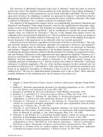
Even with only three bars in one stage, which represents the simplest form of a three-dimensional
tensegrity unit, various types of tensegrities can be constructed depending on how these bars have
been held in space to form a beam that satisfies the definition of tensegrity. Three variations of a
3-bar per stage structure are described below.
17.4.1.1 3-Bar SVD Class 1 Tensegrity
A typical two-stage 3-bar SVD tensegrity is shown in Figure 17.43(a) in which the bars of the
bottom stage are twisted in the counter-clockwise direction. As is seen in Figure 17.42 and

Figure 17.43(a), these tensegrities are constructed by using all three types of strings, saddle strings
(S), vertical strings (V), and the diagonal strings (D), hence the name SVD tensegrity.
17.4.1.2 3-Bar SD Class 1 Tensegrity
These types of tensegrities are constructed by eliminating the vertical strings to obtain a stable
equilibrium with the minimal number of strings. Thus, a SD-type tensegrity only has saddle (S)
and the diagonal strings (D), as shown in Figure 17.42 and Figure 17.43(b).
lllFIGURE 17.42 Unfolded tensegrity architecture.
FIGURE 17.43 Types of structures with three bars in one stage. (a) 3-Bar SVD tensegrity; (b) 3-bar SD tensegrity,
(c) 3-bar SS tensegrity.
(a) (b) (c)
8596Ch17Frame Page 364 Friday, November 9, 2001 6:33 PM
© 2002 by CRC Press LLC
17.4.1.3 3-Bar SS Class 2 Tensegrity
It is natural to examine the case when the bars are connected with a ball joint. If one connects
points P and P′ in Figure 17.42, the resulting structure is shown in Figure 17.43(c). The analysis
of this class of structures is postponed for a later publication.
The static properties of a 3-bar SVD-type tensegrity is studied in this chapter. A typical two-
stage 3-bar SVD-type tensegrity is shown in Figure 17.44 in which the bars of the bottom stage
are twisted in the counter-clockwise direction. The coordinate system used is also shown in the
same figure. The same configuration will be used for all subsequent studies on the statics of the
tensegrity. The notations and symbols, along with the definitions of angles α and δ, and overlap
between the stages, used in the following discussions are also shown in Figure 17.44.
The assumptions related to the geometrical configuration of the tensegrity structure are listed
below:
1. The projection of the top and the bottom triangles (vertices) on the horizontal plane makes
a regular hexagon.
2. The projection of bars on the horizontal plane makes an angle α with the sides of the base
triangle. The angle α is taken to be positive (+) if the projection of the bar lies inside the
base triangle, otherwise α is considered as negative (–).
3. All of the bars are assumed to have the same declination angle δ.

4. All bars are of equal length, L.
17.4.2 Existence Conditions for 3-Bar SVD Tensegrity
The existence of a tensegrity structure requires that all bars be in compression and all strings be
in tension in the absence of the external loads. Mathematically, the existence of a tensegrity system
must satisfy the following set of equations:
(17.129)
For our use, we shall define the conditions stated in (17.129) as the “tensegrity condition.”
Note that A of (17.129) is now a function of α, δ, and h, the generalized coordinates, labeled q
generically. For a given q, the null space of A is computed from the singular value decomposition
of A.
36,37
Any singular value of A smaller than 1.0 × 10
–10
was assumed to be zero and the null
vector t
0
belonging to the null space of A was then computed. The null vector was then checked
against the requirement of all strings in tension. The values of α, δ, and h that satisfy (17.129)
FIGURE 17.44 Top view and elevation of a two-stage 3-bar SVD tensegrity.
At() , , : .q q stable equilibrium
strings
t
00_
=>00
8596Ch17Frame Page 365 Friday, November 9, 2001 6:33 PM
© 2002 by CRC Press LLC
yield a tensegrity structure. In this section, the existence conditions are explored for a two-stage
3-bar SVD-type tensegrity, as shown in Figure 17.44, and are discussed below.
All of the possible configurations resulting in the self-stressed equilibrium conditions for a two-
stage 3-bar SVD-type tensegrity are shown in Figure 17.45. While obtaining Figure 17.45, the

length of the bars was assumed to be 0.40 m and L
t
, as shown in Figure 17.44, was taken to be 0.20 m.
Figure 17.45 shows that out of various possible combinations of α–δ–h, there exists only a small
domain of α–δ–h satisfying the existence condition for the two-stage 3-bar SVD-type tensegrity
studied here. It is interesting to explore the factors defining the boundaries of the domain of α–δ–h.
For this, the relation between α and h, δ and h, and also the range of α and δ satisfying the existence
condition for the two-stage 3-bar SVD-type tensegrity are shown in Figures 17.45(b), (c), and (d).
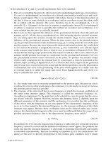
Figure 17.45(b) shows that when α = 30°, there exists a unique value of overlap equal to 50% of
the stage height. Note that α = 0° results in a perfect hexagonal cylinder. For any value of α other
than 0°, multiple values of overlap exist that satisfies the existence condition. These overlap values
for any given value of α depend on δ, as shown in Figure 17.45(c). It is also observed in
Figure 17.45(b) and (c) that a larger value of negative α results in a large value of overlap and a
FIGURE 17.45 Existence conditions for a two-stage tensegrity. Relations between (a) α, δ, and the overlap, (b)
α and overlap, (c) δ and overlap, and (d) δ and α giving static equilibria.
8596Ch17Frame Page 366 Friday, November 9, 2001 6:33 PM
© 2002 by CRC Press LLC
larger value of positive α results in a smaller value of overlap. Note that a large value of negative
α means a “fat” or “beer-barrel” type structure, whereas larger values of positive α give an
“hourglass” type of structure. It can be shown that a fat or beer-barrel type structure has greater
compressive stiffness than an hourglass type structure. Therefore, a tensegrity beam made of larger
values of negative α can be expected to have greater compressive strength.
Figure 17.45(d) shows that for any value of δ, the maximum values of positive or negative α are
governed by overlap. The maximum value of positive α is limited by the overlap becoming 0% of
the stage height, whereas the maximum value of negative α is limited by the overlap becoming
100% of the stage height. A larger value of negative α is expected to give greater vertical stiffness.
Figure 17.45(d) shows that large negative α is possible when δ is small. However, as seen in
Figure 17.45(d), there is a limit to the maximum value of negative α and to the minimum δ that
would satisfy the existence conditions of the two-stage 3-bar SVD-type tensegrity. To understand
this limit of the values of α and δ, the distribution of the internal pretensioning forces in each of

the members is plotted as a function of α and δ, and shown in Figures 17.46 and 17.47.
FIGURE 17.45 (Continued)
© 2002 by CRC Press LLC
Figure 17.46 shows the member forces as a function of α with δ = 35°, whereas Figure 17.47
shows the member forces as a function of δ with α = –5°. Both of the figures are obtained for K =
1/9, and the prestressing force in the strings is equal to the force due to a maximum prestrain in
the strings ε
0
= 0.05% applied to the string which experiences maximum prestressing force. It is
seen in both of the figures that for large negative α, the prestressing force in the saddle strings and
the diagonal strings decreases with an increase in the negative α. Finally, for α below certain values,
the prestressing forces in the saddle and diagonal strings become small enough to violate the
definition of existence of tensegrity (i.e., all strings in tension and all bars in compression).
A similar trend is noted in the case of the vertical strings also. As seen in Figure 17.47, the force in
the vertical strings decreases with a decrease in δ for small δ. Finally, for δ below certain values, the
prestressing forces in the vertical strings become small enough to violate the definition of the existence
of tensegrity. This explains the lower limits of the angles α and δ satisfying the tensegrity conditions.
Figures 17.46 and 17.47 show very remarkable changes in the load-sharing mechanism between
the members with an increase in positive α and with an increase in δ. It is seen in Figure 17.46
that as α is gradually changed from a negative value toward a positive one, the prestressing force
in the saddle strings increases, whereas the prestressing force in the vertical strings decreases. These
trends continue up to α = 0°, when the prestressing force in both the diagonal strings and the saddle
strings is equal and that in the vertical strings is small. For α < 0°, the force in the diagonal strings
is always greater than that in the saddle strings. However, for α > 0°, the force in the diagonal
strings decreases and is always less than the force in the saddle strings. The force in the vertical
strings is the greatest of all strings.
FIGURE 17.46 Prestressing force in the members as a function of α.
FIGURE 17.47 Prestressing force in the members as a function of δ.
8596Ch17Frame Page 368 Friday, November 9, 2001 6:33 PM
© 2002 by CRC Press LLC

Figure 17.45 showing all the possible configurations of a two-stage tensegrity can be quite useful
in designing a deployable tensegrity beam made of many stages. The deployment of a beam with
many stages can be achieved by deploying two stages at a time.
The existence conditions for a regular hexagonal cylinder (beam) made of two stages for which
one of the end triangles is assumed to be rotated by an angle β about its mean position, as shown
in Figure 17.48, is studied next. The mean position of the triangle is defined as the configuration
when β = 0 and all of the nodal points of the bars line up in a straight line to form a regular hexagon,
as shown in Figure 17.48. As is seen in Figure 17.49, it is possible to rotate the top triangle merely
by satisfying the equilibrium conditions for the two-stage tensegrity. It is also seen that the top
triangle can be rotated merely by changing the overlap between the two stages. This information
can be quite useful in designing a Stewart platform-type structure.
17.4.3 Load-Deflection Curves and Axial Stiffness as a Function of the
Geometrical Parameters
The load deflection characteristics of a two-stage 3-bar SVD-type tensegrity are studied next and
the corresponding stiffness properties are investigated.
FIGURE 17.48 Rotation of the top triangle with respect to the bottom triangle for a two-stage cylindrical hexagonal
3-bar SVD tensegrity. (a) Top view when β = 0, (b) top view with β, and (c) elevation.
FIGURE 17.49 Existence conditions for a cylindrical two-stage 3-bars SVD tensegrity with respect to the rotation
angle of the top triangle (anticlockwise β is positive).
8596Ch17Frame Page 369 Friday, November 9, 2001 6:33 PM
© 2002 by CRC Press LLC
Figure 17.50 depicts the load-deflection curves and the axial stiffness as functions of prestress,
drawn for the case of a two-stage 3-bar SVD-type tensegrity subjected to axial loading. The axial
stiffness is defined as the external force acting on the structure divided by the axial deformation
of the structure. In another words, the stiffness considered here is the “secant stiffness.”
Figure 17.50 shows that the tensegrity under axial loading behaves like a nonlinear spring and
the nonlinear properties depend much on the prestress. The nonlinearity is more prominent when
prestress is low and when the displacements are small. It is seen that the axial stiffnesses computed
for both compressive and tensile loadings almost equal to each other for this particular case of a
two-stage 3-bar SVD-type tensegrity. It is also seen that the axial stiffness is affected greatly by

the prestress when the external forces are small (i.e., when the displacements are small), and
prestress has an important role in increasing the stiffness of the tensegrity in the region of a small
external load. However, as the external forces increase, the effect of the prestress becomes negligible.
The characteristics of the axial stiffness of the tensegrity as a function of the geometrical parameters
(i.e., α, δ) are next plotted in Figure 17.51. The effect of the prestress on the axial stiffness is also
shown in Figure 17.51. In obtaining the Figure 17.51, vertical loads were applied at the top nodes of
the two-stage tensegrity. The load was gradually increased until at least one of the strings exceeded its
elastic limit. As the compressive stiffness and the tensile stiffness were observed to be nearly equal to
each other in the present example, only the compressive stiffness as a function of the geometrical
parameters is plotted in Figure 17.51. The change in the shape of the tensegrity structure from a fat
profile to an hourglass-like profile with the change in α is also shown in Figure 17.51(b).
The following conclusions can be drawn from Figure 17.51:
1. Figure 17.52(a) suggests that the axial stiffness increases with a decrease in the angle of
declination δ (measured from the vertical axis).
2. Figure 17.51(b) suggests that the axial stiffness increases with an increase in the negative
angle α. Negative α means a fat or beer-barrel-type structure whereas a positive α means
an hourglass-type structure, as shown in Figure 17.51(b). Thus, a fat tensegrity performs
better than an hourglass-type tensegrity subjected to compressive loading.
3. Figure 17.51(c) suggests that prestress has an important role in increasing the stiffness of
the tensegrity in the region of small external loading. However, as the external forces are
increased, the effect of the prestress becomes almost negligible.
FIGURE 17.50 Load deflection curve and axial stiffness of a two-stage 3-bar SVD tensegrity subjected to axial
loading.
(a) (b)
8596Ch17Frame Page 370 Friday, November 9, 2001 6:33 PM
© 2002 by CRC Press LLC
17.4.4 Load-Deflection Curves and Bending Stiffness as a Function of the
Geometrical Parameters
The bending characteristics of the two-stage 3-bar SVD tensegrity are presented in this section.
The force is applied along the x-direction and then along the y-direction, as shown in Figure 17.52.

The force is gradually applied until at least one of the strings exceeds its elastic limit.
The load deflection curves for the load applied in the lateral are plotted in Figure 17.52 as a
function of the prestress. It was observed that as the load is gradually increased, one of the vertical
strings goes slack and takes no load. Therefore, two distinct regions can be clearly identified in
Figure 17.52. The first region is the one where none of the strings is slack, whereas the second
region, marked by the sudden change in the slope of the load deflection curves, is the one in which
at least one string is slack. It is seen in Figure 17.52 that in contrast to the response of the tensegrity
subjected to the vertical axial loading, the bending response of the tensegrity is almost linear in
the region of tensegrity without slack strings, whereas it is slightly nonlinear in the region of
tensegrity with slack strings. The nonlinearity depends on the prestressing force. It is observed that
the prestress plays an important role in delaying the onset of the slack strings.
The characteristics of the bending stiffness of the tensegrity as a function of the geometrical
parameters (i.e., α, δ) are plotted next in Figures 17.53 and 17.54. Figure 17.53 is plotted for lateral
force applied in the x-direction, whereas Figure 17.54 is plotted for lateral force applied in the
y-direction. The effect of the prestress on the bending stiffness is also shown in Figures 17.53 and
17.54. The following conclusions about the bending characteristics of the two-stage 3-bar tensegrity
could be drawn from Figures 17.53 and 17.54:
1. It is seen that the bending stiffness of the tensegrity with no slack strings is almost equal in
both the x- and y-directions. However, the bending stiffness of the tensegrity with slack
string is greater along the y-direction than along the x-direction.
2. The bending stiffness of a tensegrity is constant and is maximum for any given values of α, δ,
and prestress when none of the strings are slack. However, as soon as at least one string goes
FIGURE 17.51 Axial stiffness of a two-stage 3-bar SVD tensegrity for different α, δ, and pretension.
(a) (b) (c)
8596Ch17Frame Page 371 Friday, November 9, 2001 6:33 PM
© 2002 by CRC Press LLC
slack (marked by sudden drop in the stiffness curves in Figures 17.53 and 17.54), the stiffness
becomes a nonlinear function of the external loading and decreases monotonically with the
increase in the external loading. As seen in Figures 17.53 and 17.54, the onset of strings becoming
slack, and hence the range of constant bending stiffness, is a function of α, δ, and prestress.

3. Figures 17.53(a) and 17.54(a) suggest that the bending stiffness of a tensegrity with no slack
strings increases with the increase in the angle of declination δ (measured from the vertical
axis). The bending stiffness of a tensegrity with a slack string, in general, increases with
increase in δ. However, as seen in Figure 17.53(a), a certain δ exists beyond which the
bending stiffness of a tensegrity with slack string decreases with an increase in δ. Hence,
tensegrity structures have an optimal internal geometry with respect to the bending stiffness
and other mechanical properties.
4. Figures 17.53(b) and 17.54(b) suggest that the bending stiffness increases with the increase
in the negative angle α. As negative α means a fat or beer-barrel-type structure whereas a
positive α means an hourglass-type structure, a fat tensegrity performs better than an hour-
glass-type tensegrity subjected to lateral loading.
5. Figures 17.53(a,b) and 17.54(a,b) indicate that both α and δ play a very interesting and
important role in not only affecting the magnitude of stiffness, but also the onset of slackening
of the strings (robustness to external disturbances). A large value of negative α and a large
value of δ (in general) delay the onset of slackening of the strings, thereby increasing the
range of constant bending stiffness. However, a certain δ exists for which the onset of the
slack strings is maximum.
FIGURE 17.52 Load deflection curve of a two-stage 3-bar SVD tensegrity subjected to lateral loading, (a) loading
along x-direction, and (b) loading along y-direction.
(a) (b)
8596Ch17Frame Page 372 Friday, November 9, 2001 6:33 PM
© 2002 by CRC Press LLC
6. Figures 17.53(c) and 17.54(c) suggest that prestress does not affect the bending stiffness of
a tensegrity with no slack strings. However, prestress has an important role in delaying the
onset of slack strings and thus increasing the range of constant bending stiffness.
17.4.5 Summary of 3-Bar SVD Tensegrity Properties
The following conclusions could be drawn from the present study on the statics of a two-stage
3-bar SVD-type tensegrities.
1. The tensegrity structure exhibits unique equilibrium characteristics. The self-stressed equi-
librium condition exists only on a small subset of geometrical parameter values. This con-

dition guarantees that the tensegrity is prestressable and that none of the strings is slack.
2. The stiffness (the axial and the bending) is a function of the geometrical parameters, the
prestress, and the externally applied load. However, the effect of the geometrical parameters
on the stiffness is greater than the effect of the prestress. The external force, on the other
hand, does not affect the bending stiffness of a tensegrity with no slack strings, whereas it
does affect the axial stiffness. The axial stiffness shows a greater nonlinear behavior even
FIGURE 17.53 Bending stiffness of a two-stage 3-bar SVD tensegrity for different α, δ, and pretension. L-bar
for all cases = 0.4 in.
(a) (b) (c)
8596Ch17Frame Page 373 Friday, November 9, 2001 6:33 PM
© 2002 by CRC Press LLC
up to the point when none of the strings are slack. The axial stiffness increases with an
increase in the external loading, whereas the bending stiffness remains constant until at least
one of the strings go slack, after which the bending stiffness decreases with an increase in
the external loading.
3. Both the axial and the bending stiffness increase by making α more negative. That is, both
the axial and the bending stiffness are higher for a beer-barrel-type tensegrity. The stiffness
is small for an hourglass-type tensegrity.
4. The axial stiffness increases with a decrease in the vertical angle, whereas the bending
stiffness increases with an increase in the vertical angle. This implies that the less the angle
that the bars make with the line of action of the external force, the stiffer is the tensegrity.
5. Both the geometrical parameters α and δ, and prestress play an important role in delaying
the onset of slack strings. A more negative α, a more positive δ, and prestress, all delay the
onset of slack strings, as more external forces are applied. Thus, both α and δ also work as
a hidden prestress. However, there lies a δ beyond which an increase in δ hastens the onset
of slack strings, as more external force is applied.
FIGURE 17.54 Bending stiffness of a two-stage 3-bar SVD tensegrity for different α, δ, and pretension.
(a) (b) (c)
8596Ch17Frame Page 374 Friday, November 9, 2001 6:33 PM
© 2002 by CRC Press LLC

17.5 Concluding Remarks
Tensegrity structures present a remarkable blend of geometry and mechanics. Out of various
available combinations of geometrical parameters, only a small subset exists that guarantees the
existence of the tensegrity. The choice of these parameters dictates the mechanical properties of
the structure. The choice of the geometrical parameters has a great influence on the stiffness.
Pretension serves the important role of maintaining stiffness until a string goes slack. The geomet-
rical parameters not only affect the magnitude of the stiffness either with or without slack strings,
but also affect the onset of slack strings. We now list the major findings of this chapter.
17.5.1 Pretension vs. Stiffness Principle
This principle states that increased pretension increases robustness to uncertain disturbances. More
precisely, for all situations we have seen (except for the C4T2):
When a load is applied to a tensegrity structure, the stiffness does not decrease as the loading
force increases unless a string goes slack.
The effect of the pretension on the stiffness of a tensegrity without slack strings is almost negligible.
The bending stiffness of a tensegrity without slack strings is not affected appreciably by prestress.
17.5.2 Small Control Energy Principle
The second principle is that the shape of the structure can be changed with very little control energy.
This is because shape changes are achieved by changing the equilibrium of the structure. In this
case, control energy is not required to hold the new shape. This is in contrast to the control of
classical structures, where shape changes required control energy to work against the old equilibrium.
17.5.3 Mass vs. Strength
This chapter also considered the issue of strength vs. mass of tensegrity structures. We found planar
examples to be very informative. We considered two types of strength: the size of bending forces
and the size of compressive forces required to break the object. We studied the ratio of bending
strength to mass and compression strength to mass. We compared this for two planar structures,
one the C2T4 unit and the other a C4T1 unit, to a solid rectangular bar of the same mass.
We find:
• Reasonably constructed C2T4 units are stronger in bending than a rectangular bar, but they
are weaker under compression.
• The C2T4 has worse strength under compression than a solid rectangular bar.

• The simple analysis we did indicates that C4T2 and C4T1 structures with reasonably chosen
proportions have larger compression strength-to-mass ratios than a solid bar.
• On the other hand, a C4T1, while strong (not easily broken), need not be an extremely stiff
structure.
• C4T2 and C4T1 structures can be designed for minimal mass subjected to a constraint on
both strength and stiffness.
It is possible to amplify the effects stated above by the use of self-similar constructions:
• A 2D Tensegrity Beam. After analyzing a C2T4 tensegrity unit, we lay n of them side by
side to form a beam. In principle, we find that one can build beams with arbitrarily great
bending strength. In practice, this requires more study. However, the favorable bending
properties found for C2T4 bode well for tensegrity beams.
8596Ch17Frame Page 375 Friday, November 9, 2001 6:33 PM
© 2002 by CRC Press LLC
• A 2D Tensegrity Column. We take the C4T2 structure and replace each bar with a smaller C4T1
structure, then we replace each bar of this new structure by a yet smaller C4T1 structure. In
principle, such a self-similar construction can be repeated to any level. Assuming that the strings
do not fail and have significantly less mass than the bars, we find that we have a class of tensegrity
structures with unlimited compression strength-to-mass ratio. Further issues of robustness to
lateral and bending forces have to be investigated to ensure practicality of such structures.
The total mass including string and bars (while preserving strength) can be minimized by a finite
numer of self-similar iterations, and the number of iterations to achieve minimal mass is usually
quite small (less that 10). This provides an optimization of tensegrity structures that is analytically
resolved and is much easier and less complex than optimization of classical structures. We empha-
size that the implications of overlapping of the bars were not seriously studied.
For a special range of geometry, the stiffness-to-mass ratio increases with self-similar iterations.
For the remaining range of geometry the stiffness-to-mass ratio decreases with self-similar itera-
tions. For a very specific choice of geometry, the stiffness-to-mass ratio remains constant with self-
similar iterations.
Self-similar steps can preserve strength while reducing mass, but cannot preserve stiffness while
reducing mass. Hence, a desired stiffness bound and reconciliation of overlapping bars will dictate

the optimal number of iterations.
17.5.4 A Challenge for the Future
In the future, the grand challenge with tensegrity structures is to find ways to choose material and
geometry so that the thermal, electrical, and mechanical properties are specified. The tensegrity
structure paradigm is very promising for the integration of these disciplines with control, where
either strings or bars can be controlled.
Acknowledgment
This work received major support from a DARPA grant monitored by Leo Christodoulou. We are
also grateful for support from DARPA, AFOSR, NSF, ONR, and the Ford Motor Company.
Appendix 17.A Nonlinear Analysis of Planar Tensegrity
17.A.1 Equations of Static Equilibrium
17.A.1.1 Static Equilibrium under External Forces
A planar tensegrity under external forces is shown in Figure 17.A.1, where F
i
are the external forces
and t
i
represent the internal forces in the members of the tensegrity units. Note that t represents
the net force in the members which includes the pretension and the force induced by the external
forces. The sign convention adopted herein is also shown in Figure 17.A.1, where t
ki
represents the
member force t acting at the i-th node of the member k. We assume that i < j and t
ki
= –t
kj
. With
this convention, we write the force equilibrium equations for the planar tensegrity.
The equilibrium of forces in the x-direction acting on the joints yields the following equations
(17.A.1)

tt t F
ttt F
ttt F
ttt F
ixix
ix
jxix
ix
ixix
jx
jxjx
jx
114 4
66
1
1122
55
2
2233
66
3
3344
55
4
cos cos cos
cos cos cos
cos cos cos
cos cos cos
δδδ
δδδ

δδδ
δδδ
++=
++=−
++ =−
++=
,
,
,

8596Ch17Frame Page 376 Friday, November 9, 2001 6:33 PM
© 2002 by CRC Press LLC
Similarly, the equilibrium of forces in the y-direction acting on the joints yields the following
equations
(17.A.2)
In the above equations, cos δ
xk
represents the direction cosine of member k taken from the x-axis,
whereas cos δ
yk
represents the direction cosine of member k taken from the y-axis.
The above equations can be rearranged in the following matrix form:
At = f, (17.A.3)
where t is a vector of forces in the members and is given by t
T
= [t
1
t
2
t

3
t
4
t
5
t
6
], matrix A (of size
8 × 6) is the equilibrium matrix, and f is a vector of nodal forces. For convenience, we arrange t
such that the forces in the bars appear at the top of the vector, i.e.,
t
T
= [t
bars
t
strings
] = [t
5
t
6
t
1
t
2
t
3
t
4
]. (17.A.4)
Matrix A and vector f are given by

(17.A.5)
In the above equation, matrices H
x
and H
y
are diagonal matrices containing the direction cosines
of each member taken from the x-axis or y-axis, respectively, i.e., H
xii
= cos δ
xi
and H
yii
= cos δ
yi
.
FIGURE 17.A.1 Forces acting on a planar tensegrity and the sign convention used.
tt t
ttt
ttt
ttt
iyiy
iy
jyiy
iy
iyiy
jy
jyjy
jy
114 4
66

1122
55
2233
66
3344
55
0
0
0
0
cos cos cos
cos cos cos
cos cos cos
cos cos cos
δδδ
δδδ
δδδ
δδδ
++=
++=
++ =
++=
,
,
,
.

A
C0
0C

H
H
f
f
f
=




















=











T
T
x
y
x
y
M
LLL
M
LL,.
8596Ch17Frame Page 377 Friday, November 9, 2001 6:33 PM
© 2002 by CRC Press LLC
Similar to the arrangement of t, H
x
and H
y
are also arranged such that the direction cosines of bars
appear at the top of H
x
and H
y
whereas the direction cosines of strings appear at the bottom of H
x

and H
y
. Vectors f
x
and f
y
are the nodal forces acting on the nodes along x- and y-axes, respectively.
Matrix C is a 6 × 4 (number of members × number of nodes) matrix. The k-th row of matrix C
contains –1 (for i-th node of the k-th member), +1 (for j-th node of the k-th member) and 0. Matrix
C for the present case is given as
(17.A.6)
It should be noted here that matrix A is a nonlinear function of the geometry of the tensegrity unit, the
nonlinearity being induced by the matrices H
x
and H
y
containing the direction cosines of the members.
17.A.2 Solution of the Nonlinear Equation of Static Equilibrium
Because the equilibrium equation given in (17.A.3) is nonlinear and also A (of size 8 × 6) is not
a square matrix, we solve the problem in the following way.
Let be the member forces induced by the external force f, then from (17.A.3)
(17.A.7)
where e is the deformation from the initial prestressed condition of each member, and from Hooke’s
law = Ke, where K is a diagonal matrix of size 6 × 6, with K
ii
= (EA)
i
/L
i
. (EA)

i
and L
i
are the
axial rigidity and the length of the i-th member. Note that A expressed above is composed of both
the original A
0
and the change in A
0
caused by the external forces f.
A = A
0
+ Ã (17.A.8)
where à is the change in A
0
caused by the external forces f.
The nonlinear equation given above can be linearized in the neighborhood of an equilibrium. In
the neighborhood of the equilibrium, we have the linearized relationship,
(17.A.9)
Let the external force f be gradually increased in small increments (f
k
= f
k-1
+ ∆f at the k-th step),
and the equilibrium of the planar tensegrity be satisfied for each incremental force, then (17.A.7)
can be written as
A(u
k
)KA (u
k

)
T
u
k
= f
k
– A(u
k
)t
0
(17.A.10)
The standard Newton–Raphson method can now be used to evaluate u
k
of (17.A.10) for each
incremental load step ∆∆
∆∆
f
k
. The external force is gradually applied until it reaches its specific value
C =
−
−
−
−
−
−































0101
10 10
1100
0110

0011
1001
Bars
Strings
˜
t
At f
At t f
At f At
AKe f At
=
⇒+=
⇒=−
⇒=−
()
0
0
0
˜
˜
˜
t
eAu
kk
T
k
=
8596Ch17Frame Page 378 Friday, November 9, 2001 6:33 PM
© 2002 by CRC Press LLC
and u

k
is evaluated at every load step. Matrix A, which is now a nonlinear function of u, is updated
during each load step.
To compute the external force that would be required to buckle the bars in the tensegrity unit,
we must estimate the force being transferred to the bars. The estimation of the compressive force
in the bars following full nonlinear analysis can be done numerically. However, in the following
we seek to find an analytical expression for the compressive force in the bars. For this we adopt a
linear and small displacement theory. Thus, the results that follow are valid only for small displace-
ment and small deformation.
8596Ch17Frame Page 379 Friday, November 9, 2001 6:33 PM
© 2002 by CRC Press LLC
Appendix 17.B Linear Analysis of Planar Tensegrity
17.B.1 EI of the Tensegrity Unit with Slack Top String
17.B.1.1 Forces in the Members
A tensegrity with a slack top string does not have prestress. As mentioned earlier, we adopt the
small displacement assumptions, which imply that the change in the angle δ due to the external
forces is negligible. Therefore, in the following, we assume that δ remains constant. The member
forces in this case are obtained as
(17.B.1)
The strain energy in each of the members is computed as
(17.B.2)
The total strain energy is then obtained as
(17.B.3)
where K is defined as
(17.B.4)
tF
tF
t
tF
t

F
t
F
1
2
3
4
5
6
2
0
=
=
=
=
=−
=−
,
,
,
,
.
tan ,
tan
cos
cos
δ
δ
δ
δ

U
LF
EA
U
LF
EA
U
U
LF
EA
U
LF
EA
U
LF
EA
s
s
s
b
b
1
0
2
2
0
2
3
4
0

2
5
0
2
6
0
2
1
2
4
1
2
0
1
2
1
2
1
2
=
=
=
=
=
=
()
,
()
,
,

()
,
()
,
()
.
tan
tan
cos
cos
3
3
3
3
δ
δ
δ
δ
UU
L
EA
F
K
i
s
i
== + +
∑
1
2

2
2
0
2
()
[],
cos
sin cos
3
33
δ
δδ
K
EA
EA
s
b
=
()
()
.
8596Ch17Frame Page 380 Friday, November 9, 2001 6:33 PM
© 2002 by CRC Press LLC
Thus, large values of K mean that the strings are stiffer than the bars, whereas small values of K
mean that the bars are stiffer than the strings. K → 0 means bars are rigid.
17.B.1.2 External Work and Displacement
External work W is given by
(17.B.5)
where u is the displacement as shown in Figure 17.11.
Equating the total strain energy given by (17.B.3) to the work done by the external forces given

by (17.B.5), and then solving for u yields
(17.B.6)
17.B.1.3 Effective EI
Because EI = Mρ, we have
(17.B.7)
Substitution of from (17.B.6) into (17.B.7) yields
(17.B.8)
Substituting L
0
= L
bar
cos δ in (17.B.7) and (17.B.8) yields the following expressions for the
equivalent bending rigidity of the planar section in terms of the length of the bars L
bar
,
(17.B.9)
or equivalently,
(17.B.10)
WFuFu==4
1
2
2,
u
FL
EA
K
s
=++
0
2

2
()
[].
cos
sin cos
3
33
δ
δδ
EI FL
L
u
=






0
0
2
2
tan tan
1
δδ.
˜
u
EI
LEA

K
s
=
++
1
22
0
2
3
( ) cos
( cos )
.
sin
sin
2
3
δδ
δδ
EI FL
L
u
bar
bar
=







sin cos sin
1
δδδ
2
2
.
EI
LEA
K
bar
s
=
++
1
22
2
3
()
(sin )
.
sin cos
cos
23
3
δδ
δδ
8596Ch17Frame Page 381 Friday, November 9, 2001 6:33 PM
© 2002 by CRC Press LLC
Appendix 17.C Derivation of Stiffness of the C4T1
i

Structure
17.C.1 Derivation of Stiffness Equation
For a C4T1
i
structure under the buckling load F, the compressive load of bar in the i-th iteration is
(17.C.1)
Similarly, the tension of strings in the i-th iteration is
(17.C.2)
So, the buckling load F can be written in terms of any one of the compressive bar loads or tension
of strings in i-th iteration
(17.C.3)
From the geometry of the structure,
(17.C.4)
Equation (17.C.3) can be simplified to
(17.C.5)
From this,
(17.C.6)
This means the force-to-length ratio of every compressive or tensile members is the same. It is
assumed that all the bars and strings have constant stiffness and, hence, are linear. With this
assumption,
(17.C.7)
So (17.C.6) becomes
(17.C.8)
F
F
i
j
i
j
=

=
∏

cos
1
2 δ
.
t
F
jii
j
j
s
j
s
==−
=
∏
2
2
123 1
1
sin
for

δ
δcos
, , , , , .
FF
t

jii
is
j
j
p
p
j
s
i
== =−
==
∏∏
2
2
21231
11
cos
sin
for δ
δ
δcos , , , , , .
sin δ
δ
j
tj
j
j
j
j
L

L
L
L
=
=
−
2
2
1
,
cos .
FF
L
L
t
L
L
i
i
j
tj
==
00
.
F
L
F
L
t
L

t
L
i
i
j
tj t0
1
1
== =.
FkL L
tkLL
i
bi
ii
jtjtjtj
=−
=−
(),
().
0
0
k
L
L
k
L
L
k
L
L

bi
i
i
tj
tj
tj
t
t
t
0
0
1
10
1
11 1−






=−






=−







.
8596Ch17Frame Page 382 Friday, November 9, 2001 6:33 PM
© 2002 by CRC Press LLC
Taking the infinitesimal of all the length quantities yields
and hence,
(17.C.9)
From the geometry of the structure,
(17.C.10)
Taking the infinitesimal of (17.C.10), noting that L
i
is length of bars, yields
(17.C.11)
Combining the (17.C.11) with (17.C.9) yields
(17.C.12)
From (17.C.5), it is natural to choose F in terms of the tension in the first iteration, i.e.,
The derivative of F w.r.t. L
0
yields
(17.C.13)
With (17.C.12), the stiffness of C4T1
i
will be
(17.C.14)
−= =k
L

L
dL k
L
L
dL k
L
L
dL
bi
i
i
itj
tj
tj
tj t
t
t
t
0
2
0
2
1
10
1
2
1
,
dL
kL

kL
L
L
dL
dL
kL
kL
L
L
dL
i
tt
bi
i
i
t
t
tj
tt
tj tj
tj
t
t
=−
=
110
0
2
1
2

1
110
0
2
1
2
1
,
.
LLL
LL L
LL
t
tt
i
i
j
tj
j
i
0
2
1
2
1
2
2
2
2
2

1
2
212
1
4
44
44
=−
=−−
=
=−
−
=
∑
()

.
dL
L
L
dL
L
LdL
i
i
i
j
tj tj
j
i

0
00
1
1
4
1
4=−
−
=
∑
.
dL
dL
kL
LL
L
kL
L
kL
t
tt
t
i
i
bi
i
j
tj
tj tj
j

i
0
1
110
01
2
3
0
1
3
0
1
44=+








−
=
∑
.
Ft
L
L
k
L

L
L
t
t
t
t
==−






1
0
1
1
10
1
0
1.
dF
dL
k
L
L
kL
L
L
dL

dL
t
t
t
t
t
t
t
0
1
10
1
10
10
1
2
1
0
1=−






+ .
K
dF
dL
k

L
L
L
L
kL
L
kL
k
L
L
k
k
L
L
L
L
k
it
t
t
i
i
bi
i
j
j
i
tj
tj tj
t

t
t
i
t
bi
i
i
i
j
t
=− = −






++








=−







+






+
−
=
−
−
∑
0
1
10
1
0
2
3
0
1
1
3
0
1
1

10
1
1
00
2
1
1
14 4
14 4
kk
L
L
L
L
tj
tj
tj
tj
j
i
00
2
1
1

























=
−
∑
.
8596Ch17Frame Page 383 Friday, November 9, 2001 6:33 PM
© 2002 by CRC Press LLC
17.C.2 Some Mathematical Relations in Buckling Design
In the strength-preserving design, the C4T1
i
system is designed to buckle at the same load as the
original bar C4T1
0

. The angles δ
j
, where j = 1, 2, …, i–1, i are free variables to be specified to fix
the geometry. Therefore, it is important to find out all the lengths and ratio quantities in terms of
these angles.
17.C.2.1 Length of Structure and Strings
From the geometry of the structure, it can be shown that
(17.C.15)
17.C.2.2 Computing the Stiffness Ratio of Strings,
Consider the ratio
From (17.109)
With (17.C.2) and (17.C.15), the ratio can be simplified to
From this,
(17.C.16)
In particular, if E
tj
= E
t
and σ
tj
= σ
t
, then
(17.C.17)
LL
LL
is
i
s
tj i j s j

i
s
01
1
2
22
=
=
=
=+
∏
∏
cos ,
sin cos .
δ
δδ
k
k
for s j i i
ts
tj
, , , , , ,=−123 1
k
k
EA
L
L
EA
E
E

r
r
L
L
tj
tj
tj tj
tj
tj
tj tj
tj
tj
tj
tj
tj
tj
() ()()
()
() ()
()
.
+++
+
++
+
=
=













111
1
11
2
2
1
π
π
k
k
E
E
t
t
L
L
t
j
tj
tj
tj

tj j
tj j
tj
tj
() ()
() ()
.
++ +
++
=












11 1
11
σ
σ
k
k
E
E

tj
tj
tj
tj
tj
tj
() ()
()
.
++
+
=






11
1
σ
σ
k
k
E
E
ts
tj
ts tj
tj ts

=
σ
σ
.
k
k
ts
tj
= 1.
8596Ch17Frame Page 384 Friday, November 9, 2001 6:33 PM
© 2002 by CRC Press LLC
So, in the strength-preserving design, if the same material is used, then all strings have the same
stiffness.
17.C.2.3 Computing the Stiffness Ratio of String to Bar
The stiffness of bar and strings are defined by
where E is the Young’s modulus, A is the cross-section area, and L is the length of bar or strings
at the buckling load. With this definition and (17.C.16),
From (17.106), (17.109), and (17.C.15),
Substitute F from (17.66) into the above equation to obtain
(17.C.18)
For some materials of bars and strings, (17.C.18) reduces to
(17.C.19)
17.C.2.4 Computing the Rest Length-to-Length Ratio of Strings, L
tj0
/L
tj
The tension in the strings is given by
k
k
jii

tj
bi
where =−123 1, , , , ,
k
EA
L
= ,
k
k
k
k
k
k
E
E
Er
L
L
Er
E
ELL
L
r
r
tj
bi
tj
ti
ti
bi

tj ti
ti tj
ti ti
ti
i
i
tj ti
itj tii
i
i
ti
i
==
=






σ
σ
π
π
σ
σ
2
2
2
2

2
1
.
k
k
E
E
tl
L
E
E
F
L
E
E
l
tj
bi
tj ti
itj
i
ti
i
ii
tj ti
itj
i
ti s
i
si i

i
p
i
p
=












=

























==
σ
σπσ δ
σ
σ
δ
πσ δ δ δ
4
2
2
2
21
2
2
2
1
2
0

1
2
1
1
2
0
sin
sin
cos sin cosΠΠ
22
.
k
k
E
l
E
E
tj
bi
tj
tj i
s
s
i
=







=
∏
π
σ
δ
2
0
2
0
1
1
2
16
2 cos .
k
k
E
l
tj
bi
tj
tj
s
s
i
=







=
∏
π
σ
δ
2
0
2
1
1
2
16
2 cos .
8596Ch17Frame Page 385 Friday, November 9, 2001 6:33 PM
© 2002 by CRC Press LLC
From (17.109),
So,
(17.C.20)
17.C.2.5 Computing the Rest Length to Length Ratio of Bars, L
i0
/L
i
From (17.C.6),
Hence,
leading to
(17.C.21)
Using (17.C.20) and (17.C.21) reduces to

(17.C.22)
17.C.2.6 Computing the String Stiffness, k
t1
Recall that the string stiffness is given by
Using (17.66), (17.108), and (17.109) yields
tkLL
t
Er
L
LL
jtjtjtj
j
tj tj
tj
tj tj
=−
=−
(),
().
0
2
0
π
t
Et
L
LL
j
tj j
tj tj

tj tj
=−
σ
().
0
L
LE
tj
tj
tj
tj
0
1=−
σ
.
F
L
t
L
i
it
=
1
1
k
L
L
k
L
L

bi
i
i
t
t
t
0
1
10
1
11−






=−






L
L
k
k
L
L

io
i
t
bi
t
t
=+ −






11
1
10
1
.
L
L
k
kE
i
i
t
bi
t
t
0
11

1
1=+
σ
.
k
Er
L
t
t
tt
t
1
11
2
1
2
0
2
1
1
161
=
=+
π
.
8596Ch17Frame Page 386 Friday, November 9, 2001 6:33 PM
© 2002 by CRC Press LLC