Electrical Engineering Mechanical Systems Design Handbook Dorf CRC Press 2002819s_14 pptx

pick-and-place industrial systems positioned by mechanical stops. For such devices pneumatic
actuation represents a fast, cheap, and reliable solution.
The hydraulic actuator is to some extent similar to the pneumatic one but avoids its main
drawbacks. The uncompressible hydraulic oil flows through a cylinder and applies pressure to the
piston. This pressure force causes motion of the robot joint. Control of motion is achieved by
regulating the oil flow. The device used to regulate the flow is called a servovalve. Hydraulic systems
can produce linear or rotary actuation. There are many advantages of the hydraulic drives. Its main
benefit is the possibility of producing a very large force (or torque) without using geartrains. At
the same time, the effector attached to the robot arm allows high concentration of power within
small dimensions and weight. This is due to the fact that some massive parts of the actuator, like
the pump and the oil reservoir, are placed beside the robot and do not load the arm. With hydraulic
drives it is possible to achieve continuous motion control. The drawbacks one should mention are:
Hydraulic power supply is inefficient in terms of energy consumption
Leakage problem is present.
A fast-response servovalve is expensive.
If the complete hydraulic system is considered (reservoir, pump, cylinder and valve), the power
supply becomes bulky.
Electric motors (electromagnetic actuators) are the most common type of actuators in robots
today. They are used even for heavy robots for which some years ago hydraulics was exclusive.
This can be justified by the general conclusion that electric drives are easy to control by means of
a computer. This is especially the case with DC motors. However, it is necessary to mention some
drawbacks of electromagnetic actuation. Today, motors still rotate at rather high speed. Rated speed
is typically 3000 to 5000 r.p.m. At the same time, the output motor torque is small compared with
the value needed to move a robot joint. For instance, rated torque for a 250W DC motor with rare-
earth magnets may be 0.9 Nm. Hence, electric motors are in most cases followed by a reducer
(gear-box), a transmission element that reduces speed and increases torque. It is not uncommon
for a large reduction ratio to be needed (up to 300). The always present friction in gear-boxes
produces loss of energy. The efficiency (output to input power ratio) of a typical reducer, the
Harmonic Drive, is about 0.75. The next problem is backlash that has a negative influence on robot
position accuracy. Similar problems may arise from the unsatisfactory stiffness of the transmission.

An important question concerns the allocation of the motor on the robot arm. To unload the arm
and achieve better static balance, motors are usually displaced from the joints they drive. Motors
are moved toward the robot base. In such cases, additional transmission is needed between the
motor and the corresponding joint. Different types of shafts, chains, belts, ball screws, and linkage
structures may be used. The questions of efficiency, backlash, and stiffness are posed again. Finally,
the presence of transmission elements makes the entire structure more complex and expensive.
This main disadvantage of electric motors can be eliminated if direct drive is applied. This under-
stands motors powerful enough to operate without gearboxes or other types of transmission. Such
motors are located directly in the robot joints. Direct drive motors are used in advanced robots,
but not very often. Problems arise if high torques are needed. However, direct drive is a relatively
new and very promising concept.

5

The most widely used electromagnetic drive is the permanent magnet DC motor. Classical motor
structure has a rotor with wire windings and a stator with permanent magnets and includes brush-
commutation. There are several forms of rotors. A cylindrical rotor with iron has high inertia and
slow dynamic response. An ironless rotor consists of a copper conductor enclosed in a epoxy glass
cup or disk. A cup-shaped rotor retains the cylindrical-shaped motor while the disc-shaped rotor
allows short overall motor length. This might be of importance when designing a robot arm. A
disadvantage of ironless armature motors is that rotors have low thermal capacity. As a result,
motors have rigid duty cycle limitations or require forced-air cooling when driven at high torque

8596Ch21Frame Page 525 Tuesday, November 6, 2001 9:51 PM
© 2002 by CRC Press LLC

levels. Permanent magnets strongly influence the overall efficiency of motors. Low-cost motors
use ceramic (ferrite) magnets. Advanced motors use rare-earth (samarium-cobalt and neodymium-
boron) magnets. They can produce higher peak torques because they can accept large currents
without demagnetization. Such motors are generally smaller in size (better power to weight ratio).

However, large currents cause increased brush wear and rapid motor heating.
The main drawback of the classical structure comes from commutation. Graphite brushes and a
copper bar commutator introduce friction, sparking, and the wear of commutating parts. Sparking
is one of the factors that limits motor driving capability. It limits the current at high rotation speed
and thus high torques are only possible at low speed. These disadvantages can be avoided if wire
windings are placed on the stator and permanent magnets on the rotor. Electronic commutation
replaces the brushes and copper bar commutator and supplies the commutated voltage (rectangular
or trapezoidal shape of signal). Such motors are called brushless DC motors. Sometimes, the term
synchronous AC motor is used although a difference exists (as will be explained later). In addition
to avoiding commutation problems, increased reliability and improved thermal capacity are
achieved. On the other hand, brushless motors require more complex and expensive control systems.
Sensors and switching circuitry are needed for electronic commutation.
The synchronous AC motor differs from the brushless DC motor only in the supply. While the
electronic commutator of a brushless DC motor supplies a trapezoidal AC signal, the control unit
of an AC synchronous motor supplies a sinusoidal signal. For this reason, many books and
catalogues do not differentiate between these two types of motors.
Inductive AC motors (cage motors) are not common in robots. They are cheap, robust, and
reliable, and at the same time offer good torque characteristics. However, control of such motors
is rather complicated. Advanced vector controllers are expensive and do not guarantee the same
quality of servo-operation as DC motors. Still, it should be pointed out that these motors should
be regarded as prospective driving systems. The price of controllers has a tendency to decrease and
control precision is being improved constantly. Presently, cage AC motors are used for automated
guided vehicles, and for different devices in manufacturing automation.
Stepper motors are often used in low-cost robots. Their main characteristic is discretized motion.
Each move consists of a number of elementary steps. The magnitude of the elementary step (the
smallest possible move) depends on the motor design solution. The hardware and software needed
to control the motor are relatively simple. This is because these motors are typically run in an open-
loop configuration. In this mode the position is not reliable if the motor works under high load —
the motor may loose steps. This can be avoided by applying a closed-loop control scheme, but at
a higher price.

Let us now discuss some ideas for robot drives that are still the topic of research. First, we notice
that all the discussed actuators can be described as kinematic pairs of the fifth class, i.e., pairs that
have one degree of freedom (DOF). Accordingly, such an actuator drives a robot joint that also has
one DOF. This means that multi-DOF joints must not appear in robots, or they have to be passive.
If a multi-DOF connection is needed, it is designed as a series of one-DOF joints. However, with
advanced robots it would be very convenient if true multi-DOF joints could be utilized. As an
example, one may consider humanoid robots that really need spherical joints (for shoulder and
hip). To achieve the possibility of driving a true spherical joint one needs an actuation element that
could be called an artificial muscle. It should be long, thin, and flexible. Its main feature would be
the ability to control contraction. Although there have been many varying approaches to this problem
(hydraulics, pneumatics, materials that change the length in a magnetic field or in contact with
acids, etc.), the applicable solution is still missing.

21.1.2 DC Motors: Principles and Mathematics

DC motors are based on the well-known physical phenomenon that a force acting upon a conductor
with the current flow appears if this conductor is placed in a magnetic field. Hence, a magnetic

8596Ch21Frame Page 526 Tuesday, November 6, 2001 9:51 PM
© 2002 by CRC Press LLC

field and electrical circuit are needed. Accordingly, a motor has two parts, one carrying the magnets
(we assume permanent magnets because they are most often used) and the other carrying the wire
windings. The classical design means that magnets are placed on the static part of the motor (stator)
while windings are on the rotary part (rotor). This concept understands brush-commutation. An
advanced idea places magnets on the rotor and windings on the stator, and needs electronic
commutation (brushless motors). The discussion starts with the classical design.
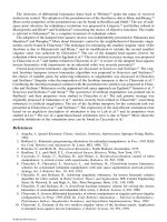
Permanent magnets create magnetic field inside the stator. If current flows through the windings
(on rotor), force will appear producing a torque about the motor shaft. Figure 21.1 shows two rotor
shapes, cylindrical and disc. Placement of magnets and finally the overall shape of the motor are

also shown.
Let the angle of rotation be

θ

. This coordinate, together with the angular velocity

,

defines the
rotor state. If rotor current is

i

, then the torque due to interaction with the magnetic field is

C

M

i

.
The constant

C

M

is known as the torque constant and can be found in catalogues. This torque has

to solve several counter-torques. Torque due to inertia is where

J

is the rotor’s moment of

FIGURE 21.1

Different rotor shapes enable different overall shape of motors.
˙
θ
J
˙˙
,θ

8596Ch21Frame Page 527 Tuesday, November 6, 2001 9:51 PM
© 2002 by CRC Press LLC

inertia and is angular acceleration. Torque that follows from viscous friction is where

B

is
the friction coefficient. Values for

J

and

B

can be found in catalogues. Finally, the torque produced
by the load has to be solved. Let the moment of external forces (load) be denoted by

M

. Very often
this moment is called the output torque. Now, equilibrium of torques gives
(21.1)
To solve the dynamics of the electrical circuit we apply the Ohm’s law. The voltage

u

supplied
by the electric source covers the voltage drop over the armature resistance and counter-electromotive
forces (e.m.f.):
(21.2)

Ri

is the voltage drop where

R

is the armature resistance.

C

E

is counter e.m.f. due to motion in
magnetic field and

C

E

is the constant. Finally,

Ldi

/

dt

is counter e.m.f. due to self-inductance, where

L

is inductivity of windings. Values

R

,

C

E

, and

L

can be found in catalogues. The dynamics of
electrical circuit introduces one new state variable, current

i

.
Equations (21.1) and (21.2) define the dynamics of the entire motor. If one wishes to write the
dynamic model in canonical form, the state vector x = [

θ

i

]

T

should be introduced. Equations
(21.1) and (21.2) can now be united into the form
(21.3)
The system matrices are
(21.4)
This is the third-order model of motor dynamics.
If inductivity

L

is small enough (it is a rather common case), the term

Ldi

/

dt

can be neglected.
Equation (21.2) now becomes
(21.5)
and the number of state variables reduces to two. The state vector and the system matrices in eq.
(21.3) are
(21.6)
The motor control variable is

u

. By changing the voltage, one may control rotor speed or position.
If the motor drives a robot joint, for instance, joint

j

, we relate the motor with the joint by using
index

j

with all variables and constants in the dynamic model (21.3). This was done in Section
20.3.1. when the motor model is integrated with the arm links model to obtain the dynamic model

of the entire robot. There the second-order model in the form of Equations (21.1) and (21.5) was
˙˙
θ
B
˙
,θ
Ci J B M
M
=++
˙˙ ˙
θθ
u Ri C Ldi dt
E
=+ +
˙
/θ
˙
θ
˙
θ
˙
xCxfMdu=+ +
CBJCJ
CL RL
fJd
L
M
E
=−
−−











=−










=











01 0
0
0
0
1
0
0
0
1
//
//
,/,
/
uRiC
E
=+
˙
θ
xC
CC RJ B J
f
J
d
CR
ME
MJ
=







=
−−






=
−






=






θ
θ

˙
,
//
,
/
,
/
00
0
0
1
0

8596Ch21Frame Page 528 Tuesday, November 6, 2001 9:51 PM
© 2002 by CRC Press LLC

applied. If the third-order model is to be used, then the canonic form of motor dynamics,
Equation (21.3), is combined with arm dynamics as explained in Section 20.3.2.
As already stated, the main disadvantage of the classical design of DC motors follows from
brush-commutation. To avoid it, brushless motors place permanent magnets on the rotor and wire
windings on the stator (Figure 21.2). The interaction between the magnetic field and the electrical
circuit, which forces the rotor to move, still exists. Brushes are not needed because there is no
current in the rotor. To synchronize switching in the electrical circuit and the angular velocity,
Hall’s sensors are used. They give the information for the device called an electronic commutator.
In this way the electronic commutator imitates the brush commutation. We are not going to discuss
the details of such a commutation system. Figure 21.2 shows the scheme of a brushless motor with
three pairs of magnetic poles and three windings.
Let us briefly discuss the voltage supplied to the windings. It is a rectangular or trapezoidal
signal switching between positive and negative values. Switching in a winding shifts with respect
to the preceding winding. Because periods of constant voltage exist, we still deal with a DC motor.

However, better performances can be achieved if a trapezoidal voltage profile is replaced with a
sinusoidal one. In this case we have a three-phase AC supply, producing a rotating magnetic field
of constant intensity. The magnetic force appears between the rotating field and the permanent
magnets placed on the rotor, causing rotor motion. The rotating field pulls the rotor and they both
rotate at the speed defined by the frequency of the AC signal. Changing the frequency, one may
control the motor speed. This concept is called the synchronous AC motor. It is clear that the
difference between a DC brushless motor and an AC synchronous motor is only in the supply.

21.1.3 How to Mount Motors to Robot Arms

When searching for the answer to the question posed in the heading, we face two criteria that
conflict with each other. First, we prefer to use direct drive motors. They eliminate transmission
and thus simplify arm construction and avoid backlash, friction, and deformation. Direct drive
motors are used in robots, but not very often. Particularly, they are not appropriate for joints that
are subject to a large gravitational load. The other criterion starts with the demand to unload the
arm. With this aim, motors are displaced from the joints they drive. Motors are moved toward the
robot base, creating better statics of the arm and reducing gravity in terms in joint torques. This
concept introduces the need for a transmission mechanism that would connect a motor with the

FIGURE 21.2

Scheme of brushless motor.

8596Ch21Frame Page 529 Tuesday, November 6, 2001 9:51 PM
© 2002 by CRC Press LLC

corresponding joint. The presence of a transmission complicates the arm design (thus increasing
the price) and introduces backlash (leading to lower accuracy when positioning some object),
friction (energy loss due to friction and problems in controlling the system with friction), and
elastic deformation (undesired oscillations). Despite all these drawbacks, some type of transmis-

sion is present in the majority of robots. It should be noted that the role of transmission is threefold.
First, power is transmitted at distance. Second, speed can be reduced and torque increased if
needed. Finally, it is possible to change the character of motion from the input to the output of
transmission system: rotation to translation (R/T) or translation to rotation (T/R). If such change
is not needed, the original character is kept: rotation (R/R) and translation (T/T). Here, we review
some typical transmission systems that appear in robots, paying attention to the three mentioned
roles of transmission.

3

Spur gearing

is an R/R transmission that has low backlash and high stiffness to stand large
moments. It is not used for transmitting at a distance, but for speed reduction. One pair of gears
has a limited reduction ratio (up to 10), and thus, several stages might be needed; however, the
system weight, friction, and backlash will increase. This transmission is often applied to the
first rotary arm axis.

Helical gears

have some advantages over spur gears. In robots, a large
reduction of speed is often required. The problem with spur gears may arise from lack of an
adequate gear tooth contact ratio. Helical gears have higher contact ratios and hence produce
smoother output. However, they produce undesired axial gear loads. The mentioned gearing
(spur and helical) is applied if the input and output rotation have parallel axes. If the axes are
not parallel, then

bevel gearing

may be applied. An example of bevel gearing in a robot wrist

is shown in Figure 21.7.

Worm gear

allows a high R/R reduction ratio using only one pair. The main drawbacks are
increased weight and friction losses that cause heat problems (e.g., efficiency less than 0.5).

Planetary gear

is an R/R transmission used for speed reduction. The reduction ratio may be
high but very often several stages are needed. Disadvantages of this system are that it is heavy
in weight and often introduces backlash. So-called zero-backlash models are rather expensive.
Note that buying a motor and a gearbox already attached to it and considering this assembly as
one unit are recommended.

Harmonic drive

is among the most common speed reduction systems in robots. This R/R
transmission allows a very high reduction ratio (up to 300 and even more) using only one pair. As
a consequence, compact size is achieved. Another advantage is small backlash, even near zero if
selective assembly is conducted in manufacturing the device. On the other hand, static friction in
these drives is high. The main problem, however, follows from the stiffness that allows considerable
elastic deformation. Such torsion in joints may sometimes compromise robot accuracy.

Cyclo reducer

is a R/R transmission that may increase the speed ratio up to 120 at one stage.
As advantages, we also mention high stiffness and efficiency (0.75 to 0.85). The main drawbacks
are heaviness and high price.

Toothed rack-and-pinion

transmission allows R/T and T/R transformation of motion. In robots,
R/T operation appears when long linear motion has to be actuated by an electric motor. The rack
is attached to the structure that should be moved and motor torque is applied to the pinion
(Figure 21.3a). The same principle may be found in robot grippers. T/R transmission can be applied
if the hydraulic cylinder has to move a revolute joint. One example, actuation of rotary robot base,
is shown in Figure 21.3b. Rack-and-pinion transmission is precise and inexpensive.

Recirculating ball nut and screw

represent a very efficient R/T transmission. It also provides
very high precision (zero backlash and high stiffness) and reliability along with great reduction of
speed. A quality ball screw is an expensive transmission. One example of a ball screw applied in
robots is presented in Figure 21.4. It is used to drive the vertical translation in a cylindrical robot.

Linkages and linkage structures

may be considered transmission elements, although they are
often structural elements as well. They feature very high stiffness and efficiency and small backlash.
In Figure 21.5 a ball screw is combined with a linkage to drive the forearm of the ASEA robot.

8596Ch21Frame Page 530 Tuesday, November 6, 2001 9:51 PM
© 2002 by CRC Press LLC

Torsion shafts or torque tubes

are R/R transmissions often used in robots to transmit power at
a distance. They do not reduce speed. The problem of torsion deformation always exists with such
systems. For this reason, it is recommended to transmit power at high speed (and low torque)

because it allows smaller diameter and wall thickness, and lower weight. An example is shown in
Figure 21.6. Wrist motors are located to create a counterbalance for the elbow. Motor power is
transmitted to the wrist by means of three coaxial torque tubes.

Toothed belts

can be found in low-cost robots. They are used to transmit rotary motion (R/R) at
long distances. It is possible to reduce rotation speed, but it is not common. The usual speed ratio
is 1:1. Toothed belt transmissions are very light in weight, simple, and cheap. The problems follow
mainly from backlash and elastic deformation that cause vibrations. Figure 21.7 shows how the

FIGURE 21.3

Toothed rack-and-pinion transmission.

FIGURE 21.4

Application of ball screw transmission to vertical linear joint of a cylindrical robot.

8596Ch21Frame Page 531 Tuesday, November 6, 2001 9:51 PM
© 2002 by CRC Press LLC

wrist can be driven by motors located at the robot base. Three belts are used for each motor to
transmit power to the joint. In the wrist, bevel gearing is applied. The combined action of two
motors can produce pitch and roll motion.

Chain

drive can replace the toothed belt for transmitting rotary motion at a distance. It has no
backlash and can be made to have stiffness that prevents vibrations. However, a chain transmission

is heavy. Chain is primarily used as an R/R transmission, but sometimes it is applied for R/T and
T/R operations.

FIGURE 21.5

Ball screw combined with a linkage transmission.

FIGURE 21.6

Wrist motors are used as a counterbalance and power is transmitted by means of coaxial torque tubes.

8596Ch21Frame Page 532 Tuesday, November 6, 2001 9:51 PM
© 2002 by CRC Press LLC

Mathematical model of transmission

. Let us discuss the mathematical representation of trans-
mission systems. If some actuator drives a robot joint, then motor motion

θ

and motor torque

M

represent the input for the transmission system. Joint motion

q

and joint torque

τ

are the output.
An ideal transmission is characterized by the absence of backlash, friction, elastic deformation
(infinite stiffness), and inertia. In modeling robot dynamics this is a rather common assumption.
In such a case, there is a linear relation between the input and the output:

q

=

θ

/N,

(21.7)

τ



=

MN

(21.8)
where

N

is the reduction ratio. This assumption allows simple integration of motor dynamics to
the dynamic model of robot links.
However, transmission is never ideal. If backlash is present, relation (21.7) does not hold.
Modeling of such a system is rather complicated, and hence, backlash is usually neglected. Friction
is an always-present effect. Neglecting it would not be justified. It is well known that static friction
introduces many problems in dynamic modeling. For this reason, friction is usually taken into
account through power loss. We introduce the efficiency coefficient

η

as the output-to-input power
ratio. Note that 0 <

η

< 1. Now, Relation (21.8) is modified. If the motion is in the direction of
the drive, then

N

η′

is used instead of

N

. However, if the motion is opposite to the action of the
drive, then

N

/

η′′

is applied. Note that

η′

and

η′′

are generally different. The efficiency of a
transmission in the reverse direction is usually smaller

η

j

′′

<

η

j

′

.
If transmission stiffness is not considered to be infinite, then the elastic deformation should be
taken into account. Relation (21.7) does not hold since

q and θ become independent coordinates.
However, stiffness that is still high will keep the values q and θ/N close to each other. To solve the
elastic deformation, one must know the values of stiffness and damping. The problem becomes
even more complex if the inertia of transmission elements is not neglected. In that case, the
FIGURE 21.7 Motors driving the wrist are located at the robot base.
8596Ch21Frame Page 533 Tuesday, November 6, 2001 9:51 PM
© 2002 by CRC Press LLC
transmission system requires dynamic modeling. One approach to this problem was presented in
Section 20.5.4.
21.1.4 Hydraulic Actuators: Principles and Mathematics
Hydraulic servoactuator consists of a cylinder with a piston, a servovalve with a torque motor, an
oil reservoir, and a pump. The term electrohydraulic actuator is also used. A reservoir and pump
are necessary for the operation of the hydraulic system, but they are not essential for explaining
operation principles. So, we restrict our consideration to the cylinder and the servovalve. The pump
is seen simply as a pressure supply. A cylinder with a piston is shown in Figure 21.8a. If the pump
forces the oil into port C
1
, the piston will move to the right and volume V
1
will increase, V
2
will
decrease and the oil will drain through port C
2
. Oil flow and the difference in pressure on the two

sides of the piston define the direction and speed of motion as well as the output actuator force.
The same principle can be used to create a rotary actuator, a hydraulic vane motor (Figure 21.8b).
We explain the servovalve operation by starting with the torque motor (magnetic motor). The
scheme of the motor is presented in Figure 21.9. If current flows through the armature windings
as shown in Figure 21.9b, magnetic north will appear on side A and south on side B. Interaction
FIGURE 21.8 Hydraulic cylinder (a) and hydraulic vane motor (b).
FIGURE 21.9 Torque motor: structure and operation.
8596Ch21Frame Page 534 Tuesday, November 6, 2001 9:51 PM
© 2002 by CRC Press LLC
with the permanent magnet will turn the armature to the left. Changing the current direction will
turn the armature to the opposite side. When the armature moves, the flapper closes nozzle D
1
or D
2
.
Figure 21.10 shows the complete servovalve. Let us explain how it works.
4
Suppose that current
forces the armature to turn to the left (Figure 21.10a). The flapper moves to the right, thus closing
nozzle D
2
. The pressure supply line is now closed and the oil from the left line, , flows
through pipe C
1
into the cylinder. The actuator piston moves to the right. Pipe C
2
allows the oil to
flow out from the cylinder to the return line R (back to the reservoir). Since nozzle D
2
is closed,

FIGURE 21.10 Operation of a servovalve.
P
s
2
P
s
1
8596Ch21Frame Page 535 Tuesday, November 6, 2001 9:51 PM
© 2002 by CRC Press LLC
the oil in the right supply line exerts strong pressure upon the right-hand side of the servovalve
piston forcing it to move to the left. This motion causes deformation of the feedback spring. At
some deformation, the elastic torque of the deformed spring starts to turn the armature to the right
and the flapper to the left, thus opening nozzle D
2
. When the oil begins to flow through D
2
, the
pressure acting upon the right-hand side of the piston reduces, but it is still stronger than the pressure
acting upon the left-hand side. Hence, the piston continues moving to the left. The pressure on
both sides of the servovalve piston balances when the flows through D
1
and D
2
become equal. This
means the vertical position of the flapper, that is, the horizontal position of the armature (Figure
21.10b). The motion of the piston stops. In this position the motor torque equals the spring
deformation torque. Let coordinate z define the position of the servovalve piston. The equilibrium
of torques may be expressed by the relation
C
M

i = γ z (21.9)
where C
M
is the motor torque constant, i is the armature current, γ is the coefficient of elastic
deformation torque, and z expresses the magnitude of deformation. The equilibrium position z of
the servovalve corresponds to some value of oil flow and accordingly some velocity of the piston
in the actuator cylinder. Since current i can change the motor torque, and thus position z (according
to Equation (21.9)), the possibility of controlling the flow and the actuator speed is achieved.
Current i represents the control variable. One should note that after the change of the current, a
transient phase takes place before the new equilibrium is established. However, one may neglect
dynamics of the servovalve and avoid analysis of the transient phase. In such case, Equation (21.9)
is satisfied all the time and thus servovalve position z immediately follows the changes of the
current. The nonlinear static characteristic of the servovalve (flow depending on the pressure and
the piston position) has the form
(21.10)
where p
s
is the pressure in the supply line, p
d
= p
1
– p
2
is the differential pressure, sgn(z) is the sign
of the position coordinate z, ρ is the oil density, w is the area gradient of rectangular port (the rate of
change of orifice area with servovalve piston motion), and D is a dimensionless coefficient. Differential
pressure means the difference in pressures in pipes C
1
and C
2

, and at the same time, the difference in
pressure on the two sides of the actuator piston. For this reason it is often called the load pressure.
When modeling the dynamics of an actuator we assume, for simplicity, symmetry of the piston
(Figure 21.11). Let coordinate s define the position of the actuator piston. The pressures on the
two sides of the piston are p
1
and p
2
, and hence, the oil exerts the force to the piston: p
1
A – p
2
A = p
d
A,
where A is the piston area. Dynamic equilibrium of forces acting on piston gives
(21.11)
where m is the mass (total mass of the piston and load referred to the piston), B is the viscous
friction coefficient, and F is the external load force on the piston (often called the output force).
Consider now oil flow through a cylinder (Figure 21.11) and denote it by Q. It consists of three
components. The first component follows from the piston motion. It is a product of piston area and
velocity, The second component is due to leakage. Since leakage depends on pressure, we
introduce leakage coefficient c as leakage per unit pressure. There are two kinds of leakage, internal
and external, as shown in Figure 21.11. If the coefficient of internal leakage is c
i
and that of the
external is c
e
, and if the coefficient of total leakage is defined as c = c
i

+ c
e
/2, then the flow due
to leakage is cp
d
. Finally, the third component follows from oil compression. Its value is (V/4β)
Q Dwz p z p
s
d
=−
()
()
1
ρ
sgn
pA ms Bs F
d
=++
˙˙ ˙
As
˙
.
˙
,P
d
8596Ch21Frame Page 536 Tuesday, November 6, 2001 9:51 PM
© 2002 by CRC Press LLC
where V is the total volume (V = V
1
+ V

2
), and β is the compression coefficient. Total volume
includes cylinder, pipes, and servovalve. Now, the flow is
(21.12)
In this way we arrive at the mathematical model of the electrohydraulic actuator. The system
dynamics is described by Equations (21.9) to (21.12). The model is nonlinear. The system state is
defined by the three-dimensional vector x = [sp
d
]
T
. The control input is current i. The nonlinear
model may be written in canonical form
(21.13)
where we tried to find analogy with the model (21.3) used for DC motors. Model matrices are
(21.14)
If a linear model is required, the expression (21.10) should be linearized by expansion into a
Taylor series about a particular operating point K(z
K
, p
dK
, Q
K
):
(21.15)
The most important operating point is the origin of the flow-pressure curve (Q
K
= p
dK
= z
k

= 0).
In such a case relation (21.15) becomes
Q = k
1
z + k
2
p
d
(21.16)
where: k
1
= ∂Q/∂z and k
2
= ∂Q/∂p
d
are called the valve coefficients. They are extremely important
in determining stability, frequency response, and other dynamic characteristics. The flow gain k
1
FIGURE 21.11 Oil flow through a hydraulic cylinder.
QAscp
V
p
dd
=+ +
˙˙
4β
˙
s
˙
()xCxfFdxi=++

CBmAm
VA Vc
fm
dx
VDwC p zp
Ms
d
=−
−−










=−











=
−










01 0
0
04 4
0
1
0
0
0
41
//
(/) (/)
,/,
()
( / ) ( / ) ( / )( sgn( ) )
ββ
βγρ
QQ
Q

z
zz
Q
p
pp
K
K
K
d
K
ddK
−=
∂
∂
−
()
+
∂
∂
−
()
© 2002 by CRC Press LLC
has a direct influence on system stability. The flow-pressure coefficient k
2
directly affects the
damping ratio of valve–cylinder combination. Another useful quantity is the pressure sensitivity
defined by k
p
= ∂p
d

/∂z = k
1
/k
2
. The pressure sensitivity of valves is quite high, which accounts for
the ability of valve–cylinder combinations to break away large friction loads with little error. If
(21.16) is used instead of (21.10), dynamic model (21.13) becomes linear with system matrices
(21.17)
Model (21.13) in its linear or nonlinear form can be combined with arm dynamics, as explained
in Section 20.3.2, to obtain the dynamic model of the complete robot system.
21.1.5 Pneumatic Actuators: Principles and Mathematics
A pneumatic servoactuator (often called a electropneumatic actuator) consists of an electropneumatic
servovalve and a pneumatic cylinder with a piston. Figure 21.12 presents the scheme of the actuator.
Let us explain how it operates.
5
Numbers 1 and 2 in the figure indicate an independent source of
energy: (1) gas under pressure with (2) a valving and pressure reduction group. An electromechanical
converter (3), a kind of torque motor, transforms the electrical signal (voltage u that comes from the
amplifier) into an angle of its output shaft (angle α). The nozzle fixed to the shaft turns by the same
angle. A mechanical-pneumatic converter (4) provides the difference in pressure and flow in chambers
(a) and (b) proportional to the angle of the nozzle. The electromechanical converter and the mechan-
ical-pneumatic converter together form the servovalve. The pneumatic cylinder (5) is supplied with
differential pressure (p
d
) and flow (Q
d
), and hence, the piston moves. Thus, the voltage applied to the
electromechanical converter represents the actuator-input variable that offers the possibility of con-
trolling piston motion. Feedback is realized by using a sliding potentiometer (6). The potentiometer
FIGURE 21.12 Scheme of a pneumatic servoactuator.

CBmAm
VA V k c
fmd
Vk C
M
=−
−
()()
−
()










=−











=
()
()










01 0
0
04 4
0
1
0
0
0
4
21
//
//
,/,
//ββ β γ
8596Ch21Frame Page 538 Tuesday, November 6, 2001 9:51 PM
© 2002 by CRC Press LLC

provides for voltage proportional to piston displacement. This is analog information describing the
position of the piston. The information is used to form the error signal by subtracting this position
from the referent position. The error signal is amplified and then applied to the electromechanical
converter. In this way the closed-loop control scheme is obtained.
Let us describe the dynamics of the pneumatic servoactuator mathematically. We first find the
relation between the input and the output of the electromechanical converter. If the inductivity of
the coil is neglected, the input voltage u reduces to:
u = R
c
i (21.18)
where R
c
is the resistance of the circuit and i is the current. If the dynamics of the rotating parts
(rotor, shaft, nozzle) is neglected, the output angle α will be proportional to the current:
α = K
i
i (21.19)
where K
i
is the coefficient of proportionality.
The flow through the mechanical-pneumatic converter is
Q
d
= K
α
α + K
p
p
d
(21.20)

where p
d
is the differential pressure (in two chambers), K
α
is the flow gain coefficient with respect
to angle α, and K
p
is the flow gain coefficient with respect to pressure.
Now we consider the cylinder. Let the coordinate s define the position of the piston. Flow through
the pneumatic cylinder can be described by the relation
(21.21)
where M is the molecular mass of gas, p
s
is the supply pressure, ζ is the pressure-loss coefficient,
R is the universal gas constant, T
s
is the supply temperature, A is the active piston area, k is the
polytropic exponent, V
0
is the total volume. Dynamic equilibrium of forces acting on piston gives
(21.22)
where m is the total piston mass (including rod and other load referred to the piston), B is the
viscous friction coefficient, and F is the external load force on the piston (often called the output
force). Note that there may exist other forces like dry friction (F
fr
sgn ) or linear force (cs). In
such cases Equation (21.22) has to be augmented.
Equations (21.18) to (21.22) describe the dynamics of the electropneumatic actuator. If the
equations are rearranged, canonical form of the dynamic model can be obtained. The system state
is defined by the three-dimensional vector x = [sp

d
]
T
. The control variable is voltage u. Equations
(21.18) to (21.22) can be united in the linear matrix model
(21.23)
where model matrices are
(21.24)
Q
Mp A
RT
s
MV
kRT
p
d
s
ss
d
=+
ζ
˙˙
0
pA ms Bs F
d
=++
˙˙ ˙
˙
s
˙

s
˙
xCxfFdu=+ +
CBmAm
p Ak V RT kK MV
fmd
RT kK K MV R
ssp sic
=−
−










=−











=










01 0
0
0
0
1
0
0
0
00 0
//
//
,/,
/ζ
α
8596Ch21Frame Page 539 Tuesday, November 6, 2001 9:51 PM
© 2002 by CRC Press LLC
Model (21.23) can be combined with the arm dynamics, as explained in Section 20.3.2, to obtain
the dynamic model of the complete robot system.

It should be said that electropneumatic servosystems cannot be applied practically for servodrives
of robotic manipulators. This is because all gases to be applied as driving media are compressible,
i.e., their specific volume is pressure dependent. In this way elasticity is introduced into the driving
system. Under a load, especially in cases of longer strokes, large loads, and big pneumatic cylinders,
this phenomenon leads to oscillations of loaded links of manipulator chain, thus rendering the
electropneumatic drives practically unusable for robotic servodrives. This is a real situation present
on the market and industry today. Pneumatic drives are applied in simple pick-and-place industrial
systems positioned by mechanical stops.
The other variants of driving units need more extensive presentation.
21.2 Computer-Aided Design
As the number of industrial robots used in manufacturing systems increases and robots tend to
be used in many nonindustrial fields, additional functions and performance improvements, such
as high speed motion and high precision positioning, are desirable. It is, however, difficult to
design robots by the conventional method of experimentation and trial manufacturing because
robots involve many design parameters and evaluation functions. Accordingly, computer-aided
design (CAD) is significant for designing suitable robots for objective tasks and saving manpower,
time, and costs required for design.
21.2.1 Robot Manipulator Design Problem
Designing a robot manipulator (or robot) requires a determination of all design parameters of its
mechanism.
• Fundamental mechanism:
1. Degrees of freedom (D.O.F.)
2. Joint types (rotational/sliding)
3. Arm lengths and offsets
• Inner mechanism:
1. Motor allocations
2. Types of transmission mechanisms
3. Motors
4. Reduction gears and their reduction ratios
5. Arm cross-sectional dimensions

6. Machine elements
The designed robot should have suitable functions and abilities to perform certain tasks. The
following design functions must be evaluated:
• Kinematic evaluation:
1. Workspace
2. Joint operating range
3. Maximum workpiece velocity and acceleration
4. Maximum joint velocity and acceleration
• Static/dynamic evaluation:
1. Maximum motor driving torque
2. Total motor power
3. Total weight
8596Ch21Frame Page 540 Tuesday, November 6, 2001 9:51 PM
© 2002 by CRC Press LLC
4. Weight capacity
5. Maximum deflection
6. Minimum natural frequency
The relationship between design parameters and evaluation functions is shown in Table 21.1. It
shows that kinematics strongly depends on fundamental mechanism, while dynamics depends on
inner mechanism.
Many robot CAD systems have been developed throughout the world.
6-18
Among them is
TOCARD (total computer-aided robot design), which has the ability to design robots comprehen-
sively and will be explained later.
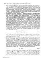
21.2.2 Robot Design Procedure
Figure 21.13 shows the total robot design procedure in this CAD system. First, the operator
(designer) inputs the design conditions which are prescribed by the objective tasks. Then, the
procedure consists of three design systems — fundamental mechanism design, inner mechanism
design, and detailed structure design, described as follows:

1. Fundamental mechanism design is based on kinematic evaluation — workspace, joint
displacement, velocity and acceleration, and workpiece velocity and acceleration.
2. Inner mechanism design requires determination of motor allocations and the types of trans-
mission mechanisms. The arm cross-sectional dimensions are calculated roughly, and the
machine elements including the motors and the reduction gears are selected from their catalog
data temporarily, based on rough evaluation of dynamics — motor driving torque, total motor
power, total weight, weight capacity, and deflection.
3. Detailed structure design involves modification of the arm cross-sectional dimensions and
reselection of the machine elements based on precise evaluation of dynamics — total weight,
deflection, and natural frequency.
TABLE 21.1 Relationship between Design Parameters and Evaluation Functions
Evaluation Function
Kinematics Dynamics Both
Design Parameter
Workspace
Joint Disp.
Limit
Max. Joint
Vel./Acc.
Max. Workpiece
Vel./Acc.
Max. Motor
Torque
Total Motor
Power
Total
Weight
Weight
Capacity
Deflection

Natural
Frequency
Positioning
Accuracy
Cost
Fundamental Mechanism
D.O.F. ∀∆∆∆∆⅜⅜ ∆ ⅜⅜⅜∀
Joint type ∀ ⅜ ∆∆∆⅜⅜ ∆ ⅜⅜⅜∀
Arm length ∀∆∀∀∀∀∀∀∀∀∀⅜
Offset ∀∀∆∆∆∆∆⅜ ∆∆∆∆
Inner Mechanism
Motor allocation ∆∆∆∆∀∀∀∀∆∆∆∆
Trans. mech. ∆∀∆∆∆∆∀∆∀∀∀∀
Motor ∆∆∀∀∀∀∀∀∆∆∆∀
Reduction gear ∆∆∀∀∀∀∀∀∀∀∀∀
Arm cross. dim. ∆∆∆∆∀∆∀∀∀∀∀⅜
Machine element ∆∆∆∆∀∆∀∀∀∀∀⅜
∀ = strong, ⅜ = medium, ∆ = weak.
Source: Modified from Inoue, K., et al., J. Robotics Soc. Jpn., 14, 710, 1996. With permission.
8596Ch21Frame Page 541 Tuesday, November 6, 2001 9:51 PM
© 2002 by CRC Press LLC
Some of the design parameters are locally optimized in each system. However, if sufficient
performance cannot be obtained in a system, the operator returns back to the previous system and
tries the previous design again. The CAD system is an interactive design system; the operator can
repeatedly alternate between design change and evaluation. The details of the above-mentioned
design systems are described in the following sections.
FIGURE 21.13 Total robot design procedure in TOCARD. (Modified from Inoue, K. et al., J. Robotics Soc. Jpn.,
14, 710, 1996. With permission.)
START
1)

design condition input
4)
kinematic analysis
5)
kinematic evaluation
OK?
OK?
3)
input of DOF, arm lengths & offsets
OK?
END
input of motor allocations
7)
& transmission mechanisms
8)
machine elements based on evaluation
estimation of arm cross. dim. &
of strength, power or deflection
9)
dynamic analysis
total motor power & deflection
evaluation of total weight
10)
sensitivity
analysis
12)
automatic
arm cross. dim.
optimization of
14)

13)
modification of
machine elements
arm cross. dim. &
dynamic analysis
15)
evaluation of total weight
16)
deflection & natural frecuency
2)
robot type selection
y
n
n
y
fundamental mechanism designinner mechanism design
n
y
deatained structure design
6)
11)
17)
8596Ch21Frame Page 542 Tuesday, November 6, 2001 9:51 PM
© 2002 by CRC Press LLC
21.2.3 Design Condition Input
21.2.3.1 Step 1
The operator inputs the design conditions or constraints prescribed by the objective tasks:
1. Sizes and weights of workpieces (including end-effectors)
2. Reference trajectories of workpieces
3. Required working space

4. Allowable deflection and natural frequency
21.2.4 Fundamental Mechanism Design
The kinematic design parameters of a robot that is a serial link mechanism as shown in Figure 21.14,
are called the “fundamental mechanism:”
1. Degrees of freedom
2. Joint types (rotational/sliding)
3. Arm lengths and offsets
The fundamental mechanism is determined based on kinematic evaluation.
21.2.4.1 Step 2
The type of robot mechanism — how rotational or sliding joints are serially arranged — is called
robot type, and most industrial robots are classified into the following categories:
• Cartesian robot (or rectangular robot)
• Cylindrical robot
• Spherical robot (or polar robot)
• Articulated robot
• SCARA robot
Generally, a robot design expert selects a suitable robot type for the objective tasks from these
categories, using empirical knowledge concerning the characteristics of the performance of each
robot type. Here a new method is introduced for selecting the most suitable robot type for the
tasks from the typical six-D.O.F. industrial robot types based on rough evaluation of the perfor-
mances using fuzzy theory. In this method, the performances of robot types derived from the
design expert’s knowledge are roughly compared with the performances required for the tasks
FIGURE 21.14 Fundamental mechanism of robot.
arm
length
arm
length
J
1
J

2
J
3
J
4
J
5
J
6
J
k
= rotational
joint
DOF = 6
8596Ch21Frame Page 543 Tuesday, November 6, 2001 9:51 PM
© 2002 by CRC Press LLC
using fuzzy theory.
19
The method is outlined below, where the italics in the examples are expressed
using fuzzy sets.
1. Five performances, workspace, dexterity, speed, accuracy, and weight capacity, are evaluated
in robot type selection, in the same way as a robot design expert’s method. These and the
suitability for the objective tasks of a robot type are expressed by fuzzy sets.
Example 21.1: Workspace is large.
Example 21.2: Suitability for task is very high (very suitable for task).
2. The empirical knowledge of the design expert concerning performance of each robot
type is expressed in the form of a fact. All such knowledge is stored in the system
beforehand.
Example 21.3: Workspace of articulated robot is very large.
3. The operator analyzes the tasks and obtains the performances required for them, which are

expressed as a set of rules; these rules are input by the operator.
Example 21.4: If workspace of robot type is large, it is suitable for painting task.
Example 21.5: If workspace of robot type is small, it is never suitable for painting task.
4. The suitability of each robot type for the tasks is obtained from 2 and 3 above by fuzzy
reasoning (Mamdani’s method).
Example 21.6: Articulated robot is very suitable for painting task.
5. After the suitabilities of all robot types are obtained, the operator selects the most suitable
type.
21.2.4.2 Step 3
After the robot type is selected, the operator inputs and modifies arm lengths and offsets. He can
also add new joints or can remove the joints that do not move when the robot moves along the
reference trajectories given as the design condition, thus increasing/reducing degrees of freedom.
21.2.4.3 Step 4
Once the fundamental mechanism is determined using the above two steps, then kinematic analyses
are applied to the designed mechanism.
Forward kinematics (Figure 21.15) — Forward kinematics calculates the workpiece position
and orientation R from the joint displacement vector q. Transformation matrix is often used for the
forward kinematics of a serial link manipulator; this system uses the revised transformation matrix
of the Denavit–Hartenberg method.
20
Inverse kinematics (Figure 21.15) — An efficient algorithm of inverse kinematics problem
calculating q from R was developed by Takano.
20
This algorithm is applicable to all types of a
six-DOF robot with three rotational joints in the wrist and can obtain a maximum eight sets of
solutions. Inverse kinematics is used for calculating the joint trajectories q[t] corresponding to the
workpiece reference trajectories R[t] given as the design condition.
Workspace analysis (Figure 21.15) — Evaluating the workspace generated by three joints near
the base is sufficient for the robot design. The method developed by Inoue can efficiently obtain
the boundary surface of such workspace of any type of robot, considering the joint operating range.

21
Velocity/acceleration analysis (Figure 21.16) — Luh’s algorithm
22
includes the process calcu-
lating the workpiece velocity v and acceleration a from q, , and ; it is used here.
21.2.4.4 Step 5
Kinematic performances of the designed fundamental mechanism are evaluated by:
• The workspace considering the joint operating range must cover the required working space
for the objective tasks given as the design condition (Figure 21.15).
• The joint operating range is limited by the structure of the joint. While wide joint operating
range makes workspace large, a long sliding joint makes the robot heavy, and using a
˙
q
˙˙
q
8596Ch21Frame Page 544 Tuesday, November 6, 2001 9:51 PM
© 2002 by CRC Press LLC
rotational joint with offset reduces the stiffness of the joint shaft to radial force. Thus, the
joint operating range is evaluated as described above (Figure 21.15).
• The maximum workpiece velocity and acceleration required for the objective tasks are given
indirectly as the design condition — the reference trajectories of workpieces (Figure 21.16).
• The maximum joint velocity and acceleration on the given trajectories should be as small
as possible so that the robot can be moved by small and light motors (Figure 21.16).
21.2.4.5 Step 6
The operator repeats the design change and evaluation alternately in Steps 3 through 5. If the above
interactive design fails, the operator goes back to Step 2 and selects another suitable robot type.
This procedure is repeated until the suitable fundamental mechanism is obtained.
FIGURE 21.15 Position kinematics, workspace, and joint operating range.
FIGURE 21.16 Workpiece velocity/acceleration and joint velocity/acceleration.
required

working space
k
q
<
-
<
-
q
kmin k
q
kmax
q
J
k
workspace
workpiece
R
joint variable
operating range
j
oint :
orientation
position/
reference
trajectory
k
q

k
q

.
J
k
v
a
workpiece
acceleration
velocity
acceleration
velocity
j
oint :
8596Ch21Frame Page 545 Tuesday, November 6, 2001 9:51 PM
© 2002 by CRC Press LLC
21.2.5 Inner Mechanism Design
The following design parameters are called “inner mechanism:”
1. Motor allocations (where the motors are to be attached)
2. Types of transmission mechanisms
3. Motors
4. Reduction gears and their reduction ratio
5. Arm cross-sectional dimensions
6. Machine elements (bearings, chains, bevel gears, etc.)
In the inner mechanism design, (1) and (2) are determined, (5) is calculated roughly, and (3),
(4), and (6) are selected from catalog data temporarily, based on rough evaluation of dynamics —
motor driving torque, total motor power, total weight, weight capacity, and deflection.
21.2.5.1 Step 7
As shown in Figure 21.17, a joint driving system consists of an actuator, a reduction gear, and
transmission mechanisms (if needed). Five types of driving elements used in this CAD system are
1. Motor/reduction gear element
2. Shaft element

3. Chain/sprocket element
4. Bevel gear element
5. Ball screw/nut element
We adopted motors and harmonic drives as actuators and reduction gears respectively, because
these are used in many industrial robots in the present time. Direct drive motors can be modeled
as motor/reduction gear elements without reduction gears. Ordinary belts and timing belts are dealt
with as chain/sprocket elements, because they are the same as chains kinematically, and only have
different stiffnesses and weights. In this step, the operator inputs motor allocations and types of
transmission mechanisms, as illustrated in Figure 21.18.
21.2.5.2 Step 8
Five types of arm/joint elements are used here (Figure 21.19).
1. Cylindrical arm element
2. Prismatic arm element
3. Revolute joint element (type 1)
4. Revolute joint element (type 2)
5. Sliding joint element
FIGURE 21.17 Joint driving systems of robot. (Modified from Inoue, K. et al., J. Robotics Soc. Jpn., 14, 710,
1996. With permission.)
chain/sprocket
bevel gear
motor/reduction gear
J
1
J
2
J
3
J
4
5

J
8596Ch21Frame Page 546 Tuesday, November 6, 2001 9:51 PM
© 2002 by CRC Press LLC
Because the arm cross-sectional dimensions of arm elements, the bearings used in joint elements,
and the machine elements used in driving elements are design parameters, the system roughly
calculates arm cross-sectional dimensions and selects motors, reduction gears, and machine ele-
ments (bearings, chains, bevel gears, etc.) from catalog data temporarily. This is done so that each
arm, joint, or driving element will have enough strength and stiffness against the internal force
acting on it and each motor will have enough power and torque to move the robot. In Figure 21.20,
B
i
is the i-th arm element, and f
i
is the force/moment acting on the lower arm element B
i–1
from
B
i
. If the joint element J
i
is rotational, the moment around the joint axis of f
i
is the joint driving
torque τ
i
of J
i
; if J
i
is sliding, the force in the joint axis direction of f

i
is the joint driving force,
which is converted into τ
i
with the ball screw/nut element.
1. The cross-sectional dimension of the arm element B
i
is determined to minimize the weight
of B
i
under the constraint that its deflection to the maximum value of the force/moment f
i+1
acting on B
i
from the upper arm element B
i+1
is less than its allowable deflection.
2. The weight, the position of center of gravity, and the inertia tensor of B
i
are calculated from
the determined dimension.
FIGURE 21.18 Example of designed transmission mechanisms. (From Inoue, K. et al., J. Robotics Soc. Jpn., 14,
710, 1996. With permission.)
8596Ch21Frame Page 547 Tuesday, November 6, 2001 9:51 PM
© 2002 by CRC Press LLC
FIGURE 21.19 Arm/joint elements. (Modified from Inoue, K. et al., J. Robotics Soc. Jpn., 14, 710, 1996. With
permission.)
FIGURE 21.20 Automatic design of each element in inner mechanism design.
(b) prismatic arm element(a) cylindrical arm element
arm element

arm element
(d) revolute joint element (type 2)
(c) revolute joint element (type 1)
arm element
arm element
(e) slidin
g

j
oint element
i
f
f
f
+1
i
i
: force/moment acting
on B from B
i
i
: -th joint element
i
-1
J
i
i
i
+1
i

J
i
B
B
B
: -th arm elementB
i
-1
i
8596Ch21Frame Page 548 Tuesday, November 6, 2001 9:51 PM
© 2002 by CRC Press LLC
3. The force/moment f
i
acting on the lower arm element B
i-1
from B
i
, thus the joint driving
torque τ
i
, can be obtained via the inverse dynamics of B
i
along the trajectories given as the
design condition.
4. The bearing used in the joint element J
i
is selected from the catalog data so that the bearing
may be lightest and have greater allowable radial/thrust load than the maximum value of f
i.
5. Each machine element used in the transmission mechanism of J

i
is selected from the catalog
data so that it may be lightest and have greater allowable torque than the maximum value of τ
i
.
6. The reduction ratio of the reduction gear for J
i
is determined via mechanical impedance
matching.*
7. The motor driving J
i
is selected from the catalog data so that it may be lightest and have
enough rated power and allowable torque to move J
i
.
8. Repeating the above-mentioned procedure alternately from the tip arm element to the base
arm element allows us to determine the design parameters of the elements temporarily.
21.2.5.3 Step 9
Determining all design parameters of the robot temporarily in this way permits the following
dynamic analyses.
Inverse dynamics — We expanded Luh’s algorithm so that it can be applied to robots with
transmission mechanisms as shown in Figure 21.17; the revised method can calculate both the joint
driving torque τ and the motor driving torque τ
m
when the robot motion q, , and are given.
This method can also calculate the internal force/moment f
i
acting on each arm element, which is
used in design of each element as described above.
Deflection analysis (Figure 21.21) — Generally, the stiffness of bearings in joints, reduction

gears, and transmission mechanisms is not negligible because it is less than the stiffness of arms.
Thus we developed an elastic model of a robot by the finite element method (FEM), which is
applicable to robots with transmission mechanisms and deals with the stiffness of arms as well as
that of bearings, reduction gears, and transmission mechanisms.
23,24
Using this model, we calculate
the deflection δ when the robot motions q, , and are given.
21.2.5.4 Step 10
The operator evaluates the dynamic performances of the designed robot:
Maximum motor driving torque — The maximum motor driving torque on the trajectories
given as the design condition should be as small as possible in order to use small and light motors.
FIGURE 21.21 Deflection and natural frequency.
*When the moment of inertia of motor and arm are I
m
and I
a
, reduction ratio gives the maximum
arm acceleration by the constant motor torque. It is called “mechanical impedance matching.”
δ
deflection
vibration
natural frequency
f
nI
a
I
m
=
˙
q

˙˙
q
˙
q
˙˙
q
8596Ch21Frame Page 549 Tuesday, November 6, 2001 9:51 PM
© 2002 by CRC Press LLC