Electrical Engineering Mechanical Systems Design Handbook Dorf CRC Press 2002819s_16 pptx

in (23.26), we derive the expression for the position modification which ensures the realization
of the target model in the form:
(23.28)
where is the sensitivity transfer function matrix . This control law involves
the impedance compensator:
(23.29)
and an additional nominal position feed forward term:
(23.30)
In the linearized robot control system, this control law provides equivalent effect as the computed
torque-based impedance control (Equation 23.23). Essentially, the main issue is to compensate for
dynamic effects in the forward position control in order to achieve the given target model, which
is similar to the nonlinear control (Equation 23.23) goal. The difference is that control law defined
in Equation (23.29) is based on linearized compensation techniques, which are less complex than
computation of nonlinear robot dynamics. However, the impedance compensator (Equation 23.29)
includes the inverse of position controller and the position control closed loop system
matrix . Generally these matrices depend on robot configuration. Moreover, using the inverse
compensators is not well suited in practice, since inverse systems produce large control signals,
amplify high frequency noise, and may introduce unstable pole zero cancellations.
However, as demonstrated in S
ˇ
urdilovi´c,
53
these shortcomings do not appear in industrial robots.
The performance of commercial industrial robotic systems allows significant simplification of
impedance control design and implementation. The robustness of internal position control allows
the disturbances due to interaction force and joint friction effects to be neglected. In other words,
the term from Equation 23.29 can be omitted, since the internal position controller
(Figure 23.11) significantly reduces the interaction force disturbance effects. Furthermore, due to
high gear ratios and accurate design of joint position controllers, the closed loop position control
transfer matrix is normal, diagonally dominant, and spatially rounded with good approxi-
mation. In other words, it exhibits similar performance independent of Cartesian directions, and

compliance frame selection achieves similar performance in a large workspace area (Figure 23.4).
Necessary conditions to ensure the spatial roundness and diagonal dominance of convenient
position control systems of industrial robots are derived in S
ˇ
urdilovi´c.
53
In the majority of industrial
robot systems, diagonal dominance is achieved by high transmission ratios in joints, causing
constant rotor inertia to prevail over variable inertia of the robot arm. The spatial roundness in the
joint and Cartesian space is achieved by uniform tuning of local axis position controllers. This
characteristic is illustrated in Figure 23.4 by the spherical form of the principal gain space of the
closed loop position control transfer matrix . These characteristics are important in decen-
tralized position control in order to ensure robust and uniform performance in Cartesian space.
They allow impedance control to be implemented simply, using the constant compensator .
In spite of implementation of inverse compensators, we can require that show inverse
characteristics only over some finite frequency range. To obtain a proper compensator, we can
employ a low pass filter (by inserting more poles), or utilize the low pass performance of the target
admittance . Moreover, assuming that the nominal motion exhibits slow acceleration/decel-
eration in the vicinity of constraints and during contact, which is a reliable premise due to unknown
∆x
f
∆xG G SG FS x
Fp t ps p
=
() ()
−
() ()
()
−
()

[]
−−11
0
ssss s
S
p
s
()
SIG
pp
ss
()
=−
()
GGGSGGGG
Fpt p pt r
sssss sss
s
()
=
() ()
−
() ()
()
=
() ()
−
()
−− −− −11 11 1
GSxGGx

pp r s
−−−
() ()
=
() ()
1
0
11
0
ss s s
G
r
−
()
1
s
G
p
−
()
1
s
G
r
−
()
1
s
G
p

s
()
G
p
s
()
G
F
G
p
−
()
1
s
G
t
−
()
1
s
8596Ch23Frame Page 607 Friday, November 9, 2001 6:26 PM
© 2002 by CRC Press LLC
constraints, we can also neglect the feed forward term (Equation 23.30) and thus substantially
simplify the control law:
(23.31)
where is the diagonal target end effector impedance matrix specifying the target behavior in
each compliance frame direction corresponding to Equation (23.14) and is the diagonal estimate
of the closed loop position transfer matrix, i.e., the estimation of its dominant diagonal part. The
controller (Equation 23.31) practically consists of a diagonal and, for a given task, constant com-
pensator. The above control law provides the following nominal closed loop contact behavior:

(23.32)
In other words, the controller (Equation 23.31) accurately realizes the desired target model in
the industrial robot control system. It is obvious that the role of this controller is to shape the
sensitivity transfer functions, i.e., the relationship between external interaction force disturbance
and the position tracking error according to the desired target impedance model (Equation 23.14),
without influencing the nominal position control performance in the free space. Only the sensitivity
transfer function to the interaction force sensed by the force sensor and used in the external control
loop is modified by the impedance control. The impedance controller does not influence the robust
and good perturbation rejection properties of the position controller toward other disturbance effects,
such as friction.
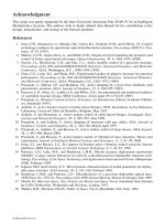
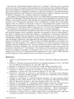
A typical result of a target model realization experiment (Figure 23.13) by the control law
(Equation 23.31) with the industrial Manutec r3 robot is presented in Figure 23.14. Obviously, a
very good match of model and experimental contact forces was achieved. The bandwidth of the
position-based impedance controller is theoretically limited by the bandwidth of the internal position
FIGURE 23.13 Target model realization experiment.
GGG
Fpt
sss
()
=
() ()
−−
ˆ
11
G
t
ˆ
G
p
xG x G F=

()
−
()
−
pt
ss
0
1
8596Ch23Frame Page 608 Friday, November 9, 2001 6:26 PM
© 2002 by CRC Press LLC
controller (commonly about 10 Hz). However, in practice, impedance controller bandwidth up to
5 Hz is reliable.
The main advantage of the position model error scheme over the force model scheme, lies in its
reliability and simpler design and implementation. The achieved system behavior is easy to understand.
Furthermore, taking into account the reliable performance of the industrial robot position control, a
sufficiently accurate and robust desired impedance behavior can be achieved with this scheme.
The position-based impedance approach in general suffers from its inability to provide soft
impedance due to limits in the accuracy of the position control system and sensor resolution. This
approach is mainly suitable for applications that require high position accuracy in some Cartesian
directions, which is accomplished by stiff and robust joint control. Design and implementation of
this scheme is simple and does not require complex computations.
The force (i.e., torque)-based approach is better suited to providing small impedance (stiffness
and damping) while reducing the contact force. From a computational viewpoint, this approach is
reasonable for applications where manipulator gravity is small and slow motion is required. In
other cases, manipulator modeling details (i.e., complete dynamic models) are needed. Contrary
to the position-based impedance control, the force-based control is mainly intended for robotic
systems with relatively good causality between joint torques and end effector forces, such as direct
drive manipulators.
23.6.1.3 Other Impedance Control Approaches
Considerable research efforts addressed the development of adaptive impedance control algorithms.

Daneshmend et al.
27
proposed a model reference adaptive control scheme with Whitney’s damping
control loop. Several authors have pursued Craig’s adaptive inverse dynamic control algorithms
54
and
expanded its application to contact motion. Lu and Goldenberg
47
proposed a sliding mode-based control
law for impedance control. The proposed controller consists of two parts: a nominal dynamic model
to compensate for nonlinearities in robot dynamics, and a compensator ensuring the impedance error
(i.e., the difference between nominal target model and the actual impedance) proceeds asymptotically
to zero on the sliding surface. In order to cope with the chattering effects in the variable structure
sliding mode control, a continuous switching algorithm in a small region around sliding surface is
proposed. Al-Jarah and Zheng
55
proposed an interesting adaptive impedance control algorithm intended
to minimize the interaction force between manipulator and environment.
FIGURE 23.14 Target model (solid) and measured (dashed) forces (improved law).
8596Ch23Frame Page 609 Friday, November 9, 2001 6:26 PM
© 2002 by CRC Press LLC
Dawson et al.
30
developed a robust position/force control algorithm based on the impedance
approach. The control scheme consists of two blocks: a desired trajectory generator computing the
modified command position based on the target impedance model and using the nominal position
and force measurements, and a controller involving a PD regulator and robust control part. The
purpose of the robust controller is to ensure that the control tracking error (i.e., the difference
between target and actual robot impedance) proceeds asymptotically to zero in spite of model
uncertainties within specified bounds. Robust control design is currently one of the most challenging

topics in controlling contact tasks.
Under some circumstances, the impedance control can be applied to achieve desired contact
forces. When an impedance-controlled manipulator is in contact with the environment, the inter-
action force is completely determined by the input position, target impedance, and the model
(impedance) of the environment. It is then apparent from Equations (23.14-15) that the interaction
forces can be precisely controlled using the impedance approach as long as an exact model of the
environment and the robot is available. By using the force-based approach in this case, the desired
force can be achieved in the open loop, and a force sensor is not needed. Such an approach is very
similar to the passive gain adjustment.
In general, however, it is difficult to exactly know the location and impedance of the environment
and robotic system. If the stiffness of the environment is much greater than the stiffness of the
target impedance and the robot, the force can also be controlled in a desired accuracy range by
using only the impedance model, rather than only knowledge about the environment.
51
When these
conditions are not fulfilled, i.e., stiffness of the environment is not much greater than that of the
target impedance, it is necessary to perform estimation experiments to obtain the model of the
environment and control the contact force. However, the on-line estimation of the environment is
complex and coupled with several practical problems: uncertain robot motion sensing at low
velocities, noise, disturbances due to friction and vibrations, impact, etc., that can significantly
influence the results. Using the robot to acquire the data for an off-line estimation is risky in
principle, and in tasks with variable environment, virtually impossible.
23.6.2 Hybrid Position/Force Control
This approach is based on a theory of compliant force and position control formalized by Mason
1
and
concerns a large class of tasks involving partially constrained motion of the robot. Depending on the
specific mechanical and geometrical characteristics of the contact problem, this approach makes a
distinction between two sets of constraints upon robot motion and contact forces. The constraints that
are natural consequences of the task configuration, i.e., of the nature of the desired contact between

an end effector held by the robot and a constrained surface, are called natural constraints. Physical
objects impose natural constraints. As already mentioned, a suitable frame in which the task to be
performed is easily described, i.e., in which constraints are specified, is referred to as the constraint
frame (or task frame or compliance frame).
56
For example, for a surface sliding contact task, it is
customary to adopt the Cartesian constraint frame as sketched in Figure 23.15. Assuming an ideal rigid
and frictionless contact between the end effector and the constraint surface, it is obvious that natural
constraints restrict end effector motion in z direction and rotations about x and y axes. The frictionless
contact prevents the forces in these directions and allows the torque around the z axis to be applied.
In order to specify the task of the robot with respect to the compliant frame, artificial constraints
must be introduced. The artificial constraints must be imposed by the control system. These
constraints essentially partition the possible DOFs of motion in those that must be position con-
trolled and those that should be force controlled in order to perform the given task. The need to
define an artificial constraint with respect to force when there is a natural constraint on the end-
effector motion in this direction (i.e., DOF) and vice versa (Figure 23.15) is obvious.
To implement hybrid position/force control, a diagonal Boolean matrix S, called the compliance
selection matrix,
7
has been introduced in the feedback loops to filter out sensed end effector forces
8596Ch23Frame Page 610 Friday, November 9, 2001 6:26 PM
© 2002 by CRC Press LLC
and displacements that are inconsistent with the contact task model. In accordance with the specified
artificial constraints, the i-th diagonal element of this matrix has the value 1 if the i-th DOF with
respect the task frame is to be force controlled and the value 0 if it is position controlled. To specify
a hybrid contact task, according to Mason,
1
the following information sets must be defined:
1. Position and orientation of the task frame
2. Denotation of position and force controlled directions with respect to the task frame (selection

matrix)
3. Desired position and force setpoints expressed in the task frame
Once the contact task is specified, the next step is to select the appropriate control algorithms. The
relevant methods are discussed below.
23.6.2.1 Explicit Force Control
The most important method within this group is certainly the algorithm proposed by Raibert and
Craig.
7
Figure 23.16 represents the control scheme that illustrates the main idea. The control consists
of two parallel feedback loops, the upper one for the position, and the lower one for the force
FIGURE 23.15 Specification of surface sliding hybrid position/force control task.
FIGURE 23.16 Explicit hybrid position/force control.
8596Ch23Frame Page 611 Friday, November 9, 2001 6:26 PM
© 2002 by CRC Press LLC
feedback loop. Each of these loops uses separate sensor systems. The positional loop utilizes the
information obtained from the positional sensors at the robot joints, and the force loop is based on
force-sensing data. Separate control laws are adopted for each loop. The central idea of this hybrid
control method is to apply two outwardly independent control loops assigned to each DOF in the
task frame. Both control loops cooperate simultaneously to control each of the manipulator joints.
This concept, at first glance, appears to be ideal for solving hybrid position/force control problems.
However, a deeper insight into the method reveals some essential difficulties and problems.
The first problem is related to the opposite requirements of the hybrid control concept concerning
position and force control subtasks. Namely, the position control must be very stiff to keep the
positioning errors in the selected directions as small as possible. The force control requires a
relatively low stiffness of the robot (corresponding to the desired force) in the force controlled
direction with respect to the task frame to ensure that the end effector behaves compliantly with
the environment. As explained above, the explicit hybrid control attempts to solve this problem by
control decoupling into two independent parts that are position and force controlled (Figure 23.16).
In the force-controlled directions, the position errors decrease to zero by multiplication with the
selection matrix orthogonal complement (position selection matrix) defined as .* This

implies that the position control part does not interfere with the force control loop, but that is not
the case. The joint space nature of robot control realization results in a coupling between position
and force control loops that are previously decoupled mathematically in the task frame. Assuming
a proportional plus differential (PD) position control law, and assuming that the force control
consists of a proportional plus integral controller (PI) with gain and , respectively, and a
force feed forward part, the control law according to the scheme in Figure 23.16 can be written in
the Cartesian space as:
(23.33)
Based on relationships between Cartesian and joint space gains, Zhang and Paul
26
proposed an
equivalent hybrid control law in the joint space:
(23.34)
Since each robot joint contributes to the control of both position and force, couplings in the
manipulator’s mechanical structure (implied in the Jacobian matrix) cause a control input to the
actuator, corresponding to the force loop (e.g., force-controlled directions) to produce additional
forces in position-controlled directions in the task frame, and vice versa. It is obvious from
Equation (23.33) that by setting the position errors in the force controlled directions to zero (i.e.,
by filtering the position error through ), the position feedback gains in all directions are changed
in comparison with the position control in free space. This causes the entire system to become
more sensitive to perturbations. As a consequence, the performance of a robot with this scheme is
not applicable for all robot configurations or all position/force-commanded directions. Moreover,
one can find certain configurations with which, depending on selected force and position directions,
the robot becomes unstable with the control law (Equation 23.33). This can be easily demonstrated
on a simplified linearized robot model, derived from Equation (23.6) by neglecting the nonlinear
Coriolis and centrifugal effects (due to small velocities in the contact task) and assuming that
gravitational effects are ideally compensated for:
*For the sake of simplicity it is assumed that the task frame coincides with the Cartesian frame. Generally the
selection matrix S is not diagonal in Cartesian space.
35

SIS=−
K
Fp
K
Fi
ττ= + + + +
∫
KS x KS x KSF KS F F
pvFp
Fi
0
∆∆∆ ∆
˙
dt
ττ
q
== + + + +
−−
∫
JkSJqkJSJqJKSFKSFF
1TT
dtτ
pv
fp fi
0
J
1
∆∆∆∆
˙
()

S
8596Ch23Frame Page 612 Friday, November 9, 2001 6:26 PM
© 2002 by CRC Press LLC
(23.35)
Let us analyze the case where the manipulator is in free space and a noncontacting environment
(e.g., in the transition phase when the force-controlled robot is approaching a contact surface after
being switched from the position-control mode). Assume that some directions (e.g., orthogonal to
the contact surface) have been selected for force control and remaining directions for position
control. Taking into account that the force is zero, substituting Equation (23.33) in Equation (23.35)
yields:
(23.36)
with a robot closed loop system matrix:
. (23.37)
To analyze the stability of this system, we determine the eigenvalues of A. As shown in Stoki´c
and S
ˇ
urdilovi´c,
57
the closed-loop matrix becomes unstable in a number of configurations. Even if
we introduce feedback loops with respect to the integrals of position errors in directions that are
position controlled, it is always possible to find unstable configurations. These unstable configura-
tions build working subspaces far away from singular positions where the system matrix A is
intrinsically unstable due to the degeneration of the Jacobian matrix. Moreover, only alterations of
the selection matrix can cause switching of robot behavior from stable to unstable and vice versa.
The kinematic instability was experimentally tested and proven using the industrial robot control
systems.
57
Although the above stability analysis was based on a linearized model and therefore has some
limitations, it provides a simple explanation of the nature of stability problems in hybrid position/force
control. Since only the robot’s position and the selection matrix influence the instability, this phenom-

enon is referred to as kinematic instability.
58
This phenomenon does not depend on whether the robot
is in contact with the constraint surface. However, in contact situations, analysis of this problem is
complicated by force/position relationship and the tests become very dangerous. It may be concluded
that the kinematic instability problem encountered in the considered explicit hybrid position/force
control represents a serious deficiency of this method and significantly reduces its applicability.
In order to overcome the difficulties related to kinematic instability, Zhang
59
proposed to introduce
an additional selection of input forces. In other words, the input torques from position and force
control parts (Figure 23.16) are decoupled in the task frame before they are applied to the joints.
When the robot is in free space, the joint torque from the position control part (Equation 23.34) is
initially transferred in the Cartesian-compliant frame, then multiplied with the selection matrix,
and again transferred back using the static force transformation (i.e., Jacobian matrix) that provides
the following control law for the position loop:
(23.38)
It is relatively easy to prove that the linearized model (Equation 23.36) becomes kinematically
stable with this control law. However, similar to the original control scheme, the eigenvalues of
the system change with variation of the robot configuration and with the given task, i.e., selection
matrix. This causes the robot performance to be strongly dependent on the configuration and
selection of controlled directions.
ΛΛττ()
˙˙
.x xF=+
ΛΛ()
˙˙ ˙ ˙
x x K Sx K Sx K Sx K Sx++= +
vp v p00
A

0I
KS KS
=






−−
ΛΛ
1111
pv
ττ
q
p
TT
p
TT
v
=+
−− −−
JSJ kJ SJ q JSJ k SJ q
11
∆∆J
˙
.
8596Ch23Frame Page 613 Friday, November 9, 2001 6:26 PM
© 2002 by CRC Press LLC
Fisher and Mujtaba

60
have shown that kinematic instability is not inherent to the explicit hybrid
position/force control scheme; it is a result of an inappropriate mathematic formulation of posi-
tion/force decomposition via selection matrix S. It was demonstrated that in the original hybrid
control formulation (Equations 23.33 and 34), the position control loop is responsible for inducing
the instability, namely the term in Equation (23.34). The crucial error in the position control
loop is, in the authors’ opinion, made by the decomposition of the robot coordinate (DOF) to
position- and force-controlled. Instead, to compute the selected position-controlled DOF and the
corresponding selected joint errors, respectively, based on:
(23.39)
and
. (23.40)
the authors proposed to use the “correct” relationship between the selected Cartesian errors and
the joint errors:
(23.41)
Taking into account the selection matrix structure, it is obvious that is a singular matrix
(with zero rows corresponding to the force DOF). Hence, the selected joint errors equivalent to the
selected Cartesian position error are obtained as the minimal 2-norm solution:
(23.42)
or, when the robot is a singular position type, or has a redundant number of joints, with an additional
term from the null space of the Jacobian :
(23.43)
where is an arbitrary vector in the joint space and the plus sign denotes the Moor–Penrose
pseudoinverse matrix. Thus, for the case in Equation (23.42), the control law of the position hybrid
control part becomes:
(23.44)
To determine how the above kinematic transformations can induce instability of the hybrid
control, the authors defined a sufficient condition for kinematic stability. From the control viewpoint,
this criterion prevents the second order system gain matrices (Equation 23.33) from becoming
negative definite, which is a condition that produces system instability.

59
By testing the kinematic
stability conditions for both original and correct selection and position error transformation solu-
tions, the authors have proven that the instability can occur in the first case. The new hybrid control
scheme, however, always satisfies the kinematic stability condition — it is always possible to find
a vector to ensure kinematic stability.
The second problem relates to dynamic stability issues in force control.
61
These effects concern
high gain effect of force sensor feedback (caused by high environment stiffness), unmodeled high
JS
J
−
1
xSx
p
=
∆∆ ∆ ∆qJxJSxJSJq
pp
===
−− −11 1
∆∆xSJq
p
=
()
SJ
()
∆∆ ∆∆∆q SJ x SJ S x SJ x SJ J q
pp
=

()
=
()
=
()
=
()
++ ++
J
∆∆qSJxIJJz
p
q
=
()
+−
[]
+
+
z
q
ττ
q
p
pv
=
()
+
()
++
kSJJqk SJJq∆∆

˙
.
z
q
8596Ch23Frame Page 614 Friday, November 9, 2001 6:26 PM
© 2002 by CRC Press LLC
frequency dynamic effects (due to arm and sensor elasticity), contact with a stiff environment,
noncollocated sensing and control, and other factors.
To overcome dynamic problems of hybrid position/force control, several researchers pursued the
idea to include the robot dynamic model in the control law. The resolved acceleration control
originally formulated for the position control
62
belongs to the group of dynamic position control
algorithms. Shin and Lee
31
extended this approach to the hybrid position/force control. The joint
space implementation of the proposed control scheme is shown in Figure 23.17. The driving torque
compensates for the gravitational, centrifugal, and Coriolis effects, and feedback gains are adjusted
according to the changes in the inertial matrix. An acceleration feed-forward term is also included
to compensate for changes of nominal motion in position directions. Finally, the control inputs are
computed by:
(23.45)
where is the commanded equivalent acceleration:
(23.46)
and is the command vector from the force control parts whose form depends on the applied
control law. To minimize the force error, it is convenient to introduce the PI force regulator of the
form:
. (23.47)
Khatib
22

introduced an active damping term into the force control part to avoid bouncing and
minimize force overshoots during transition (impact effects):
(23.48)
FIGURE 23.17 Resolved acceleration–motion force control.
ττµµ=+
()
+
()
+
∗∗
ˆ
˙˙
ˆ
,
˙
ˆ
ΛxpSfxx x
˙˙
x
∗
˙˙ ˙˙ ˙ ˙
xxKxxKxx
∗
=+ −
()
+−
()
00 0vp
f
∗

fKFFK FF
∗
=−
()
+−
()
∫
fp fi
dt
00
ττΛΛ
fvf
=−
∗
Sf SK x
ˆ
˙
8596Ch23Frame Page 615 Friday, November 9, 2001 6:26 PM
© 2002 by CRC Press LLC
where is a diagonal Cartesian damping matrix. Bona and Indri
63
proposed further modifications
of the control scheme. To compensate for the coupling between force and position control loops
and for the disturbance of the position controller due to reaction force, the authors modified the
position control law according to:
(23.49)
If the dynamic modeling used for computation of the control law is exact, the above control law
provides complete decoupling between position and force control in the task frame, i.e., the
following closed loop behavior:
(23.50)

An experimental evaluation and comparison of explicit force control strategies was presented in
Volpe and Khosla.
64
23.6.2.2 Position Based (Implicit) Force Control
The reason explicit force control methods cannot be suitably applied in commercial robotic systems
lies in the fact that commercial robots are designed as positioning devices. The feedback term, i.e.,
the signal proportional to the force errors, is multiplied by the transposition of the Jacobian matrix
in order to calculate the driving torques that have to be realized around the joints to achieve the
desired force action (Figure 23.16). These signals are directly fed to the inputs of the local servo
parts. However, the computed torques may not be accurate for commercial robotic systems. Since there
is no position feedback loop in the force-controlled direction, the robot will move due to various
disturbances acting upon it, such as controller and sensor drifts, etc.
57
The implementation of explicit
force control can be successfully performed only by a new generation of direct drive robots.
In commercial applied robotic systems, implementing implicit or position-based force control
by closing a force-sensing loop around the position controller (Figure 23.18) appears promising.
The input to the force controller is the difference between desired and actual contact force in the
task frame. The output is an equivalent position in force-controlled directions which is used as
reference input to the positional controller. According to the hybrid force/position control concept,
FIGURE 23.18 Implicit hybrid position/force control.
K
v
f
ττµµ
p
xx x=− −
()
[]
+

()
+
()
∗−∗
ˆ
˙˙
ˆ
ˆ
,
˙
ˆ
ΛΛSx Sf F p
11
˙˙ ˙˙
ˆˆ
˙
.x Sx S Sf S F SK x=+ − −
∗−∗−
ΛΛΛΛ
1111
vf
© 2002 by CRC Press LLC
the equivalent position in force direction is superimposed to the orthogonal vector in the
compliance frame, which defines the nominal position in orthogonal position-controlled directions.
The robot behavior in force direction is affected only by the acting force. The positional controller
remains unchanged, except for the additional transformations between Cartesian and task frame
which have to be introduced since these two frames are not coincident. Since a positional controller
provides a basis for realization of force control, this concept is referred to as implicit or position-
based force control,
15

or external force control.
13
The role of force control block in this scheme is two-fold, first, to compensate for the effects of
environment (contact process), and second, to achieve tracking of the desired force. Another
important quality of a force-controlled manipulator is the ability to respond to positional variations
of the contact surfaces. Commonly, a PI force controller has been applied. A more complex force
controller including the compensation of the internal position control effects has been proposed in
Stoki´c and S
ˇ
urdilovi´c.
65
In Figure 23.18 an explicit force control block is added. This scheme
combines the implicit and explicit control with the aim of using benefits (robustness and reliability
of implicit force control and fast reaction of the explicit one) and compensating specific disadvan-
tages of single force control approaches.
The main features of the implicit force control scheme are its reliability and robustness. Imple-
mented in commercial robotic systems, this scheme is neither configuration dependent nor sensitive
to parameter variation. This control algorithm can be used for arbitrary processes. However, this
scheme also exhibits some drawbacks. The accuracy of contact forces is mainly limited by the
precision of robot positioning (sensor resolution). The precision can be disturbed when contact
with a very stiff environment is requested. Fortunately, inherent compliance of the robot structure
or force sensor is always present and reduces the equivalent system stiffness. The performance of
implicit force control is significantly limited by the bandwidth of the position controller. A slightly
higher bandwidth can be achieved by using a compensator of a higher order. However, due to
coupling between position and force-controlled degrees of freedom, whether force control can
become significantly faster is questionable.
23.6.2.3 Other Force Control Approaches
The next group of algorithms considers more complex constraints on robot motion. They are
described as a set of rigid hypersurfaces in the spaces of end effector Cartesian coordinates,
11

or
in the joint coordinate space.
32
The system model is described by a typical set of linearly implicit
second order differential algebraic equations (mechanical differential algebraic equations). This
model is used to compute the control law to linearize and decouple the system dynamics and divide
the control problem into position- and force-controlled directions.
To improve reliability, the dynamic hybrid control is extended to unknown environments that
consist of hypersurfaces.
66
The improved control schemes involve on-line identification algorithms
based on force and position measurements and adaptive control mechanisms. However, the adaptive
constrained motion control is theoretically attractive, but impractical in reality. Hence, the hybrid
control algorithms become even more complex and difficult to implement in real time with the
computational and sensing resources available for robotic manipulators today.
The hybrid position/force task specification has been a subject of several investigations. Lipkin and
Duffy
24
demonstrated that Mason’s position/force decomposition approach based on geometrical
orthogonality is in fact erroneous. The resulting planning for hybrid control is not invariant with respect
to translation of origin or change of unit length. The authors proposed a more general and mathemat-
ically consistent invariant hybrid task formulation based on screw algebra. The complementarity
between motion (modeled by a twist) and force (represented by a wrench) is expressed via a reciprocity
relationship independent of coordinate frame, scaling, or units. Two fundamental relations between
twist and wrench, referred to as freedom and constraint equations, have been introduced to test task
compatibility with the model of the environment. These relations correspond to analytical expressions
for natural and artificial constraints in the noninvariant hybrid approach. For every constrained motion
x
0
F

x
0
P
8596Ch23Frame Page 617 Friday, November 9, 2001 6:26 PM
© 2002 by CRC Press LLC
task, two screw subspaces that correspond to artificial constraints can be derived. These subspaces
represent the sets of screws about which twists and wrenches can be controlled.
In certain simple tasks and reference frames, both conventional and reciprocity-based decompo-
sition show the same results. However, the reciprocity-based approach provides a more general
decomposition applicable when the freedom and constraint subspaces do not span a six-dimensional
space or have nonzero intersections and also to manipulators that have fewer than six DOF.
67
If the twist and wrench are consistent with the environment (i.e., the freedom and constraint
equations are satisfied) the specified task is feasible for hybrid control. In the opposite case, the
specified twist and wrench must be filtered to obtain a kinestatically realizable control action (so-
called kinestatic filtering).
A procedure to apply the reciprocity-based task decomposition to manipulator dynamics to obtain
equations of motion relevant for hybrid control was presented by Sinha and Goldenberg.
68
Several
model-based tools for task specification using this approach were presented by Khatib.
22
The
reciprocity concept is well suited for nominal specification of arbitrary motion constraints and also
serves to define possible uncertainties and on-line identification and observation of real motion
constraints. This strategy generally makes task execution against uncertainties very robust. This is
particularly essential for contour-following tasks. An overall hybrid position force control scheme based
on general decomposition formalism including identification of geometrical uncertainties was proposed
by De Schutter and Bruyninckx.
25

Design of appropriate controllers is subject to further researches.
23.6.3 Force/Impedance Control
Several attempts have been made to combine impedance and force control with the aim of com-
pensating for specific disadvantages of single control approaches. Although it is possible under
some circumstances to demonstrate correspondence between force and impedance control laws,
69
there are essential differences between these main constraint motion control concepts.
The main advantage of impedance control over force control is easier task specification and
programming. A contact task is specified in terms of motion sequences, so the impedance control
does not require modifications of conventional free space planning control concepts and algorithms
(the programmer can take advantage of existing off-line programming). Moreover, impedance
control can be activated in free space during approach motion. Thus, it can be applied for the
transition to and from the constraint motion, without specific control-switching algorithms.
Impedance control allows closed-loop position control in free space, while in contact with rigid
environments, it offers force open-loop capabilities. Conversely, the force (admittance) control
approach allows closed-loop force control capabilities in contact, but exhibits open-loop position
control characteristics in free space. Therefore, the activation of force control in free space is only
possible under specific circumstances. In general, however, a discontinuous control strategy is
required for the transition from noncontact to contact motion phase or vice versa. The control
structure change is done during the most critical phase when the manipulator is in contact with the
environment. That represents a major drawback of force control. To cope with unexpected collisions,
additional sensors (e.g., distance) have to be integrated into the control system. The fundamental
superiority of force control is, however, that the interaction force is the result of the control action,
rather than a result of deviation of the environment position and the chosen target impedance.
In Goldenberg’s algorithm,
38
force control is closed around an internal impedance control loop.
Desired force and force error are used to compute an equivalent desired relative motion of the end
effector. Impedance control is included with the aim of achieving a suitable relationship between
force and relative motion during contact. This is realized in the internal velocity loop by compensator

gain adjustment to obtain target impedance. A similar reliable position-based force/impedance
control scheme suitable for implementation in industrial robots has been proposed by S
ˇ
urdilovi´c
and Kirchhof.
70
An external implicit force controller loop is closed around an internal position-
based impedance controller (Figure 23.19). The main goal of the internal loop is to achieve target
8596Ch23Frame Page 618 Friday, November 9, 2001 6:26 PM
© 2002 by CRC Press LLC
impedance while the external loop takes care of desired force realization. The selection between
position (i.e., impedance) and force-controlled directions is not needed. Indeed impedance and
force control affect all directions. A disproportion between motion and force planning is not critical
in the control scheme (Figure 23.19), since the internal control loop behaves as a low stiffness
target impedance system allowing relatively large differences between input position command and
real robot position in the output. In the reverse, the internal loop in the implicit force control
(Figure 23.18) is a very stiff position control, and the selection is inevitable.
Anderson and Spong
12
proposed an approach referred to as hybrid impedance control algorithm
to control contact forces. The kernel part of the algorithm is Raibert and Craig’s hybrid posi-
tion/force control scheme, with the selection matrix applied to decompose position- and force-
controlled subspaces. Both control parts use the feedback of contact force to realize desired system
impedance (position-based and force-based impedance control) along each DOF.
A controller that combines an internal position control, a position-based impedance compensator,
and a desired force feed forward was proposed by Mayeda et al.
71
The authors suggest that integral
control actions be applied for both impedance (damping control) and force filters to ensure the
compliance and the desired steady state force.

A different approach to position/force control, referred to as parallel control (Figure 23.20), has
been proposed by Chiaverini and Sciavicco.
9
Contrary to the hybrid control, the key feature of the
parallel approach is to have both force and position controls along the same task space direction without
a selection mechanism. In general, both position and force cannot be effectively controlled in an
uncertain environment. Therefore, the logical conflict between the position and force actions is managed
by the dominance of the force control action over the position action along the constrained task direction
FIGURE 23.19 Position-based force/impedance control.
FIGURE 23.20 Parallel position/force control.
8596Ch23Frame Page 619 Friday, November 9, 2001 6:26 PM
© 2002 by CRC Press LLC
where a force interaction is expected. The force control is designed to prevail over the position control
in constrained motion directions. This means that force tracking is dominant in directions where an
interaction with the environment is expected, while the position control loop allows compliance, i.e.,
a deviation from the nominal position in order to reach the desired forces. For this reason, the parallel
control method can be considered a force/impedance control approach. The designed position tracking
quality in constrained motion directions corresponds to target impedance behavior.
A set of sufficient local asymptotic stability conditions has been derived by Chiaverini et al.
72
for a parallel controller case consisting of a PD action on the position loop and a PI control in the
force loop, together with gravity compensation and the desired force feed forward. Stability analysis
and simulation results on an industrial robot are included. These conditions imply a relatively high
damping (i.e., velocity gain) to ensure system stability.
23.6.4 Position/Force Control of Robots Interacting
with Dynamic Environment
Vukobratovi´c and Ekalo
8,33
established a unified approach to simultaneously control position and
force in an environment with completely dynamic reactions. This fully dynamic approach to the

control of robots interacting with dynamic environments will be presented in a condensed way. It
will be assumed that n = m, where n is the number of robot DOFs and m is the number of contact
force components. The general case in which n > m has been considered by Vukobratovi´c et al.
73
When the environment does not possess displacements (DOFs) that are independent of robot
motion, the environment dynamics in the robot coordinate space can be described by the model
(23.9). Then the system (23.1 through 23.9) describes the dynamics of robot interaction with a
dynamic environment. It is assumed in the contact case that all mentioned matrices and vectors are
continuous functions and that the robot is in permanent unilateral contact with the environment.
In the case of contact with the environment, the robot control task can be described as motion
along a programmed trajectory representing a twice continuous differentiable function, when
a desired force of interaction acts between the robot and the environment. The nonlinear
model programmed motion and desired force must satisfy the relation:
(23.51)
The control goal of robot interaction with a dynamic environment can be formulated by defining
the control for that is to satisfy the target conditions:
(23.52)
The two questions are addressed to the control design problem. Can we choose such a control
law that, by satisfying preset robot motion quality, would enable the attainment of the control goals
that satisfy the relation of Equation (23.52)? Is it possible to choose the control law in such a way
as to ensure the preset quality of the robot interaction force and the attainment of the control goals?
The answer to the first question is quite simple:
8,33
the inverse dynamics methods ensure that desired
motion quality is achieved and at the same time guarantee that the interaction force is stable. The
answer to the second question depends on the environment dynamics.
The task of stabilizing the programmed interaction force can be posed by considering
a family of transient responses with respect to force in the form and by choosing
a continuous vector function Q of dimension n, such that the asymptotic stability as a
whole is ensured for the trivial solution of .

q
p
t(
)
F
p
t()
q
p
t() F
p
t()
F()f(()()())
f( ) (S ( )) [M( ) L( )]
p
T1
t q tq tq t
q,q,q q q q q,q
ppp
≡
=− +
−
,
˙
,
˙˙
˙˙˙ ˙˙ ˙
.
ττ()ttt≥
0

q( ) q ( ) F( ) F ( )
pp
tttt→→ →∞,,ast
()()PFI t
p
F
µµ= −F( ) F ( )
p
tt
(() )Q 00=
µµ()t ≡ 0
8596Ch23Frame Page 620 Friday, November 9, 2001 6:26 PM
© 2002 by CRC Press LLC
Let us consider pure force control according to the assumption that , i.e., when the number
of the contact force components is equal to the number of the powered DOFs of the robot. For
convenience, when describing the quality of transient response perturbation force dynamics,
, we shall use an equivalent relation of the form:
(23.53)
With no loss in generality, we can adopt , because the stabilization of in the sense of
preset quality Equation (23.53) directs stabilization according to the preset quality inde-
pendently from the value of .
Let us consider only one of the possible control laws with the feedback loops with respect to
, and F of the form
8,33
. (23.54)
By applying this control law to the robot dynamics model Equation (23.1) we obtain the following
law of robot operating in contact with the environment:
Taking into account the environment dynamics model Equation (23.9), we obtain the following
closed-form control system:
(23.55)

and, because , (23.55) is equivalent to: , from which
follows directly. In this way, the control law (23.54) ensures the desired quality of stabilization of
.
The stability of the real motion (position) when asymptotic stability of the contact force is
fulfilled has been considered.
8,33,89–91
Sufficient conditions for contrained motion stability based on
the generalized Lyapunov’s stability theorem in the first approximation of the system with pertur-
bation have been derived. The theorem conditionally defines the internal stability properties of the
environment because the fulfillment of stability conditions depends in general not only on envi-
ronment dynamics but also on the nature of the programmed motion.
23.7 Contact Stability and Transition
The types of contact tasks may vary substantially in relation to specific requirements, but in all
cases of performing a contact task the robot must perform three kinds of motions:
• Gross motion, related to movement in free space (free motion mode)
• Compliant or fine motion, related to movement constrained by environment
• Transition motion, representing all passing phases between free and compliant motion
mn=
˙
()µµ=Q µ
˙
( ) ( ( )) .µµµµtd
t
t
=+
∫
0
Q µω ω
0
µµ

0
0≡µµ
˙
()µµ=Q µ
µµ
0
qq,
˙
ττ= − + + µ




















++−

−
∫
H( )M ( ) L( ) S ( ) F Q( ( )) h( ) g J ( )F
1
p
T
q q q q q d q,q (q) q,
˙˙
T
t
t
ωω
0
MqL S F Q(())
T
p
t
t
0
qq
()
+
()
=
()
+







∫
˙˙
˙
q,q dµω ω
S ( ) Q( ( ))d 0
T
t
t
0
qt
()
−






=
∫
µµµωω
rank S n()=µµ() ( ( ))td
t
t
=
∫
Q µω ω
0

˙
() ( ( ))µµ t = Q µω
()()PFI F t
p
8596Ch23Frame Page 621 Friday, November 9, 2001 6:26 PM
© 2002 by CRC Press LLC
The contact transition can be considered stable if the contact is not lost after the manipulator
meets the environment. A stable contact transition can be characterized by nonzero force (after
contact is detected), positive penetration of manipulator end point into environment, nonappearance
of bouncing, etc. The most critical issue in transition control is initial impact against a stiff
environment. A stable controller should ensure the passage through the transition phase and maintain
contact until all impact energy has been absorbed.
In most of the proposed control algorithms, instability occurs when the contact between end
effector and environment is stiff. However, the investigations were primarily concerned with the
question of coupled stability (i.e., will the robot remain stable when it is interconnected with the
environment?) of robots and the environment under various control algorithms, while assuming the
manipulator initially is and remains in contact with environment. Surprisingly, relatively little
research has addressed the problem of contact transition stability (i.e., will the robot during
transition from free to contact motion establish a continuous contact with the environment without
multiple impacts?) which is most fundamental for performing contact tasks. The contact transition
stability problem is important for both unilateral (force) and bilateral (geometric) constraints. A
bilateral constraint is usually achieved by closing the gripper, due to position misalignment usually
resulting from unilateral contact between gripper jaws and grasping object.
In impedance control, contact stability issues have mainly been considered based on simplified
models of interaction between a target impedance system and the environment. Colgate and Hogan
74
defined necessary and sufficient conditions to ensure the stability of a linear robotic system coupled
to a linear environment. The authors applied the network theory to describe the manipulator- and
environment-interactive behavior at the equilibrium point. For the coupled interactive system
described by the linear models, the equilibrium is defined by:

(23.56)
where and denote nominal penetration, expressing a position planning
failure due to tolerances, a desired entry into the environment, and actual robot penetration,
respectively. For the adopted linear target impedance and environment models defined by
Equations (23.14) and (23.11) respectively, these equilibriums can be expressed as:
(23.57)
Expressing the essential impedance control characteristics, interaction force F, penetration p,
and position error e, in terms of nominal penetration are useful for the analysis of both coupled
and contact transition stability.
53
During contact establishment, is a positive monotone-
increasing function. In a passive stationary environment, two time-invariant networks coupled along
interaction ports (Figure 23.21) can represent the interactive model around the equilibrium
. The coupling makes the velocities of the robot and the environment at contact point
equal, while the forces acting upon the robot and the environment have opposite activities (action
pp xx
pp xx
ee ppxx
FF
∗∗
∗∗
∗∗∗∗∗
∗
=→∞
()
=−
=→∞
()
=−
=→∞

()
=−=−
=→∞
()
tt
tt
tt
tt
;
;
;
;
e
e00 0
00
pxx
00
=−
e
pxx=−
e
FIGG GpIKK Kp
pIKK p
eIKK KKp
∗
−
−
∗
−
−

∗
∗
−
−
∗
∗
−
−
−
∗
=+
() ()
[]
()
=+
[]
=+
[]
=+
[]
et e
e
00 0
1
1
0
1
1
0
1

1
0
1
1
1
0
ˆ
et e
et
tet
p
0
t
()
pp
00
∞
()
=
∗
8596Ch23Frame Page 622 Friday, November 9, 2001 6:26 PM
© 2002 by CRC Press LLC
and reaction). If the environmental transfer matrix is positive real, representing a passive
Hamiltonian environment, then a necessary and sufficient condition to ensure stability of a linearized
robotic control system is that the realized admittance be positive real.
74
In other words,
it should represent the driving point impedance of a passive network. In a SISO system, the coupled
stability has been proven by using the Nyquist criterion and the positive real transfer function that
has a limited phase of ± 90°.

74
It is then relatively easy to prove that the mapping of the Nyquist
contour of a positive real environmental impedance through an also positive real admittance
, altering the phase by ± 90° and changing the magnitude by a factor 0 to , provides a
stable system, i.e., a stable Nyquist plot of the open-loop coupled system transfer function.
The system passivity concept provides a relatively simple test for the assessment of coupled
system stability. Only the passivity of the environment can be proven without accurate knowledge
of parameters. Assuming that the ideal target impedance response Equation (23.15) is realized, the
passivity of target admittance implies positive definite matrices , , and , and
consequently, the closed-loop system should be stable in contact with any passive environment to
which it is directly coupled. The explicit design of a positive-real robot control system, however,
may become cumbersome.
75
Moreover, various practical control implementation effects, including
computational time delay, sampling effects, and unmodeled dynamics (e.g., high order actuator and
arm dynamic effects), may result in a nonpassive real impedance control response.
75
The above stability results can be extended to nearly passive control systems. However, a passive
environment can destabilize the coupled system. To simplify coupled stability analysis, Colgate
and Hogan
74
used worst or most destabilizing environment to denote the most critical environment
for coupled system stability. Such environmental impedance shapes the Nyquist contour
of by minimizing the distance from the critical point –1 to the nearest point on the Nyquist
plot of the loop transfer function . Since the driving point impedance of simple passive
environmental models, such as mass or spring ( and ), performs the maximum rotation in
the Nyquist plane, the authors found that the worst passive environment for coupled stability consists
of a set of pure masses and springs. If both the environment and the realized admittance are stable,
the coupled stability of the interactive system in Figure 23.21 can also be assessed by means of
the small gain theorem by which a feedback loop composed of stable operators will certainly remain

stable if the product of all operator gains is smaller than unity:
(23.58)
The small gain theorem provides a general law, valid for continuous- or discrete-time, SISO and
MIMO, and linear and nonlinear systems. It is also the convergence criterion used in many iterative
FIGURE 23.21 Robot/environment interaction model.
G
e
s
s
()
ssG
t
−
()
1
G
e
ss
()
ss
ˆ
G
t
−
()
1
∞
ss
t
G

−
()
1
M
t
B
t
K
t
G
e
ss
()
ss
ˆ
G
t
−
(
)
1
GG
et
ss
() ()
−1
Ms
e
sK
e

GG
et
jjωω
() ()
<
−
∞
ˆ
1
1
8596Ch23Frame Page 623 Friday, November 9, 2001 6:26 PM
© 2002 by CRC Press LLC
processes. Furthermore, the norm inequality criterion (Equation 23.58) can easily be extended to
maintain the uncertainties in the target system and environment models.
However, the small gain theorem only provides sufficient stability conditions, which in many cases
are too conservative to be of much use in practical contact tasks. For example, assuming that ideal
second-order target impedance has been achieved, the condition (Equation 23.58) implies the admissible
target stiffness to be to ensure a stable interaction. In stiff environments, this has no practical
relevance. This result is similar to the stability analysis performed by Kazerooni et al.
16
The established
interaction stability criterion practically implies that the gain of feedback compensator (i.e., the target
admittance) should be limited by the magnitude of sum of environmental admittance and robot position
control sensitivity. For a SISO system, this imposes, in the steady state:
(23.59)
In direct drive robotic systems with significantly less position control stiffness (due to elimination
of the transmission) than in industrial robots, this condition might provide reliable target models
for practical tasks. The sufficiency of stability condition (Equation 23.59) has experimentally been
demonstrated on a lightweight direct drive University of Minnesota robot. However, from the
viewpoint of industrial robot performance, this condition is conservative and practically useless.

In industrial robots, with stiff servo gains (e.g., position control gains usually have the order 10
6
N/m), the value is and the above condition also requires the target stiffness to be higher
than the environmental one. Moreover, no target model, i.e., the compliance feedback compensator
(Figure 23.11), can be found to enable interaction with an infinitely rigid environment ( ).
Therefore, one of the main conclusions in Kazerooni et al.
16
pointed out the need for intrinsic
compliance either in the robot or in the environment to maintain interactive stability.
The coupled stability analysis around the equilibrium point cannot be applied for the analysis
of contact transition stability, and this represents a fundamental contact control task problem.
Reliable criteria ensuring contact stability of a linearized robotic control system under impedance
control during transition from the free space to a unilateral contact within a passive environment
has been established by S
ˇ
urdilovi´c.
42
The contact transition stability conditions require interaction
force, i.e., actual penetration to be nonnegative , or the position deviation to be
less than the nominal penetration i.e.,
(23.60)
This relation implies the actual end effector position during a stable contact transition will always
be located between the position of environment and the nominal position. Since this contact stability
condition is based on a simple geometric consideration, it is referred to as the geometric criterion.
42
This criterion theoretically can be applied in cases when the actual position overshoots the nominal
one, i.e., when , which provides a negative position error. However, in a contact with an
industrial robot with a realistic stiff environment, the actual motion is nearly stopped by the resistant
force and impedance control effects, so this case has no practical relevance. The advantage of the
geometric criterion is that it compares two time signals. The norm comparison offers possibilities

to apply relatively simple and efficient system theory formalisms for contact stability analysis. This
criterion has been utilized
76
to derive the robust contact stability condition ensuring both coupled
and contact transition stability based on:
(23.61)
KK
te
≥
KKK
tpe
≥
()
min ,
KK
pe
>
G
f
K
e
→
∞
pxxt
e
()
=− ≥0
eptt
()
≤

()
0
e
p
pp
p
xx
xx
t
t
tt
t
tt
t
e
()
()
=
()
−
()
()
=
()
−
()
()
−
≤
0

0
0
0
0
1
pp>
0
sup
e
p
WIG G
t
t
sss
()
()
<
()
+
() ()
()
≤
−
−
∞
2
0
2
1
1

1
et
8596Ch23Frame Page 624 Friday, November 9, 2001 6:26 PM
© 2002 by CRC Press LLC
where stable weighting transfer function matrix describes uncertainties of the environmental
model and the target impedance realization. In a SISO system, this condition implies:
(23.62)
where and are target damping and stiffness ratios, respectively. However,
in spite of an effective and simple formulation, this criterion ensures sufficient contact stability condi-
tions, but not the necessary ones. Consequently, the obtained contact stability indices might be con-
servative. It should be mentioned that the damping ratio bound Equation (23.62) is still less than the
usually applied dominant real pole solution
77
imposing . A very important advantage of the
input/output criterion Equation (23.61) is that it can be applied for both continuous and discrete systems
including the time lags. The control time lag has been identified by S
ˇ
urdilovi´c
76
as the critical desta-
bilizing contact transition effect. In general, a retarded system requires a significantly higher amount
of damping to stabilize the transition process with delayed force signals.
Typical transition experimental results in position-based impedance and force control during
contact with a stationary environment are presented in Figure 23.22.
42
The force transition in hybrid
control is characterized by lower overshoots. The reason is that force control represents an explicit
aspect of hybrid control that is achieved by appropriate control structure and design. In the
impedance control, however, the aim is to passively modify a preplanned motion in accordance
with the interaction forces. Therefore, the force transition in the impedance control is greatly

measured and influenced by selected target impedance parameters and nominal motion.
42
Lawrence
14
analyzed the destabilizing influence of time delays on impedance control perfor-
mance. Vossoughi and Donath
78
investigated the influence of nonlinear friction effects on the
performance of an impedance-controlled hand. High position control gain (or integral gain) leads
to limit cycles due to friction/stiction effects.
In contrast to the impedance control algorithms that provide the same control structure for the
three motion phases, the transition to and from contact motion is usually based on discontinuous
control in force control schemes. The change of the control strategy from position control to force
control occurs in the free space, and the transition is realized in the force control mode after contact
is established. Most force control algorithms execute the transition control in the force mode. The
reason is that the impact force can be very large, especially when due to high approach velocities
and delay in a stiff position controller. One method to reduce impact is to use a soft force sensor,
79
FIGURE 23.22 Performance comparison: impedance vs. implicit hybrid control.


W(s
)
ξκ
t
≥+−
()
1
2
12 1

ξ
ttt
= BMK
t
2 κ=KK
et
ξκ
t
≥+1
8596Ch23Frame Page 625 Friday, November 9, 2001 6:26 PM
© 2002 by CRC Press LLC
i.e., passive compliance, but this reduces the position accuracy during position control. The under-
lying idea of most methods concerned with the impact problem is to increase damping in the
collision direction.
22
Assuming a simplified stiffness model of environment, the damping effect can
be achieved either by force derivatives or approach velocity feedbacks. However, both methods
have practical limits. The force signals are usually noisy and the derivation is inaccurate. Qian and
De Schutter
80
proposed low-pass sensor filtering and nonlinear damping to cope with the transition
problem. The velocity sensing is also not reliable at slow approach motion before contact.
Moreover, in a stiff environment, relatively fast oscillations in force and velocity can cause
instability due to time (phase) lags between sensing and control action. These difficulties have been
recently addressed in several works aimed at designing a stable force controller without velocity
measurement,
81
and without end effector contact force sensing,
82
when the system dynamics is well

known. However, these innovative schemes are complex to implement and require further tests.
Independent of the active damping method, the transition control based on the force mode generally
requires some modification of control strategy or gains before and after impact. For example, in integral
explicit force control, the force error integration in the free space causes the robot to accelerate in the
force direction. Hence, the maximum impact velocity or integration wind-up should be limited in the
free space. In implicit integral force control, a constant force error corresponds to a constant position
correction velocity, but usually the different gains should be used in the free space and during contact
to achieve desired system performance. The gains synthesized for stiff contact provide very slow free
motion, while contact stability is jeopardized in the opposite case.
In the second transition control concept, the approach phase is realized in the position control
mode; after contact is established, the control is switched to force control mode. Numerous dis-
continuous transition control algorithms have recently been tested. By treating the discontinuous
controller as an entire generalized system, Mills and Lokhorst
83
proposed a discontinuous control
scheme that guarantees global asymptotic stability of the closed-loop system, asymptotic trajectory
tracking of position and force inputs, and reestablishment of contact after an inadvertent loss.
Wu et al.
84
proposed the addition of a positive acceleration feedback to the force control in the
impact direction. In addition, a switching control strategy is introduced to eliminate unexpected
bouncing. A similar control strategy for the transition problem in both force and impedance control
has been developed by Volpe and Khosla.
85
They recommended use of positive force feedback
during transition, and integral force control after stable contact is established. A force-regulated
switch triggers the transition from position control to impact control. For the further switch to
integral force control, several options were proposed. Based on the equivalency of force and
impedance control, the authors established the transition stability condition for the impedance
control-imposing ratio (robot inertia through target inertia) at less than one. Using a direct drive

robot at very high impact velocity (0.7 m/s) with a relatively stiff environment (10
4
N/m), the
authors demonstrated the reliability of established criteria. However, these results are not applicable
to industrial robots, with high Cartesian inertia levels (> 500 kg), very stiff position controllers,
and time lags that cause switching algorithms to be critical.
Gorinevski et al.
86
examined the transition problem of both impedance and general force control
during contact with stationary and dynamic environments. They tested linear control and sliding
mode control. The influence of several effects, such as time delay and elasticity of robot end effector,
transmissions and mechanical structure, on the contact stability has been examined. The contact
stability criteria for single and two DOF systems are derived in the explicit closed form in terms
of control gains and limits on robot and environments velocities.
Several authors consider transition control a short-impulse dynamic problem. This model is valid
for very fast systems (e.g., micro–macro manipulators), but is seldom used in practice. In industrial
robotic systems, the transition problem can be accurately analyzed in a finite time period. Most
industrial control systems still do not provide mechanisms to control short-impulse impact effects.
McClamroch and Wang
32
emphasized the importance of constraints in constrained dynamics. They
presented global conditions for tracking based on a modified computed torque and local conditions for
8596Ch23Frame Page 626 Friday, November 9, 2001 6:26 PM
© 2002 by CRC Press LLC
feedback stabilization using a linear controller. The closed-loop properties of force disturbances,
dynamics in the force feedback loops, and uncertainties in constrained functions were also investigated.
Eppinger and Seering
87
have studied the influence of unmodeled dynamics on contact task stability,
introducing additional (elastic) degrees of freedom of both the robot and the environment.

A treatment of the contact stability, considering the environment as a nonlinear dynamic system
is given by Hogan.
34
It is shown that if the impedance control is applied, enabling the robot to be
asymptotically stable in free space, the robot interacting with the environment is a passive system
and is stable in isolation. However, the conclusion is valid only if the robot in contact is at rest
and for this reason the result cannot be considered complete. The stability issue, i.e., the establish-
ment of the conditions under which a particular control law guarantees the stability of the robot in
contact with the environment, is of great importance.
Vukobratovi´c and Ekalo,
8,33
and Vukobratovi´c
88
focused attention on control laws that simulta-
neously stabilize the motion of the robot and the forces of its interaction with a dynamic environ-
ment, ensuring the exponential stability of the closed-loop systems (based on the analysis of a
complete dynamic model of the robot and the dynamic environment). The papers formulate con-
ditions ensuring an asymptotically stable position of the system in the first approximation (local
stability). The character of the position stability depends particularly on the nature of the pro-
grammed (desired) motion. In spite of sufficient conditions of the linearized system, asymptotic
stability is conservative, and the dynamic character of the interaction of the environment with the
robot can lead to positional instability. This problem deserves the full attention of researchers and
designers of robot controllers dedicated to diverse contact tasks. This linear analysis provides very
important criterion that must be fulfilled by any force-based law. However, the model uncertainties
representing a crucial problem in control of robots interacting with a dynamic environment still
have not been appropriately addressed. Therefore, it can be difficult to achieve the asymptotic
(exponential) stability of the system (unless robust control laws including factors for compensationg
these perturbations and uncertainties are used). Inaccuracies of robot and environment dynamic
models and dynamic control robustness have been considered by Ekalo and Vukobratovi´c.
89-91

Problems arising from parameter uncertainties may also be resolved by applying knowledge-
based techniques.
92
Taking into account external perturbations and model uncertainties, it may be
difficult to achieve asymptotic (exponential) stability. Therefore, it is of practical interest to require
less restrictive stability conditions, i.e., to consider the so-called practical stability of the system.
An approach to analysis of the practical stability of manipulation robots interacting with a dynamic
environment based on a centralized model of the system is presented by Stoki´c and Vukobratori´c.
93
The test conditions for practical stability of the robot interacting with dynamic environment are
recently derived.
93,94
The presented tests might be too conservative due to the number of lineariza-
tions (approximations) made. More refined approximations by, e.g., taking into account possible
dependencies of the model elements (matrix of inertia, Coriolis forces, Jacobian matrix, etc.) on
the parameters, may lead to less conservative tests.
23.8 Synthesis of Impedance Control at Higher Control Levels
Although several sophisticated control strategies have been proposed, the numbers of advanced
robotic contact task applications remain insignificant. The reason is that most new concepts concern
particular problems and the integration of the required algorithms and control concepts is tedious.
Most of the studies on impedance and force control relate to servo control. Except for the seminal
works on compliance control,
1,48
contact task planning and programming issues have been somewhat
neglected in the research studies.
The next section briefly addresses solving high-level impedance control problems in industrial
robotic systems. The problems with impedance control motion planning and programming layers
were investigated during the development of the new space robot control system (SPARCO),
95
in

order to develop a completely integrated reliable impedance control system including control,
8596Ch23Frame Page 627 Friday, November 9, 2001 6:26 PM
© 2002 by CRC Press LLC
programming, and monitoring functions. Several control algorithms for the integration of a position-
based impedance control scheme in conventional industrial robot control systems will be presented.
23.8.1 Compliance C-Frame
One of the most common approaches for word modeling (specification of robot and object positions)
in robot programs is based on coordinate frames. Beside coordinate frames that are convenient for
the programming of robot motion in the free space (e.g., robot base B, end point E, tool T frame,
etc.), a compliance control includes two new frames, specific for compliant motion programming:
force sensing S and compliance frame C. The S frame is a force sensor-specific frame in which
the forces and torques are measured. This frame is commonly defined relative to the robot end
point E. With respect to the C frame, the target impedance behavior (robot impedance reaction) is
specified and controlled. Since the location of the C frame depends on the current task, we have
chosen to specify the convenient C frame relative to task T frame (Figure 23.23) taking into account
that the T frame is a variable selected to meet specific task motion requirements. Usually the desired
robot position specifies the location of the T frame (specified relative to the E frame, e.g., tip of
the tool) with respect to an object frame.
The basic specification of compliance control required for the implementation addresses both
the definition of C frame location with respect to the tool frame and the selection of appropriate
target impedance parameters in the C frame based on the geometric model (Figure 23.7) for the
specific task. A set of associated robot programming commands is needed to handle this specification
in the robot program.
A specific problem in the position-based impedance control is the computation of the position
correction (Figure 23.11) corresponding to the interaction force. An obvious approach is to
compute this modification in the C frame where the compliance behavior is specified. While the
computation of for the translational DOFs is straightforward, there are several possibilities for
managing the rotational difference dependent on the representation of orientation. The description
of orientation affects the relationship between the position displacement and the
forces/torques. The form of the target impedance matrices (Equation 23.14) in Cartesian space also

depends on rotation representation. The SPARCO control system approach
95,96
utilizes the angle
axis orientation description in the C frame. The compliance model (Figure 23.7) is based on ideally
decoupled translational and rotational stiffness (impedance). This is indeed an idealized represen-
tation. As demonstrated by Lonari,
97
a point at which translational and rotational elasticity are
completely decoupled does not always exist for a compliantly supported spatial rigid body. The
point at which they are maximally decoupled is referred to as the center of stiffness. The simple
SPARCO approach allows the rotational impedance parameters to be directly related to the task
geometry described in the C frame, i.e., in the tool-frame T
0
. The selection of the C frame location
is based on geometric task analysis in T
0
and consideration of the force/displacement equilibrium.
96
FIGURE 23.23 Compliance frame and position modification.
∆x
F
∆x
F
xxpp
00
−= −
8596Ch23Frame Page 628 Friday, November 9, 2001 6:26 PM
© 2002 by CRC Press LLC
Additional possible rotation description models for compliance control are presented by Cac-
cavale et al.

98
Several authors considered achieving target stiffness with linear and rotational
springs,
99
spring systems,
100
and serial elastic mechanisms.
101
Besides the synthesis of passive
compliance devices, these works are relevant for the better understanding of spatial compliant
behavior in robot contact interaction tasks. A more general compliance planning (impedance
selection) approach has recently been proposed by Fasse and Broenink.
102
This approach is based
on spatial affine presentation of compliance described by sets of geometrical and nongeometrical
parameters independent of robot/object configuration. A spatially affine family of compliances
provides invariant wrenches with respect to the rigid body transformation. This simplifies the
selection of the target impedance.
23.8.2 Operating Modes
Additional control functions and commands are required to manage dynamic communication
between the basic position control system and the impedance control module. This section describes
impedance control functions that support programming compliance control applications.
Although the impedance control feedback is activated and deactivated by contact with the environ-
ment (Figure 23.11), the mechanisms must functionally manage the activation of the control modules
and functions. It is convenient to introduce the following impedance control operating modes:
• Stopped mode, with no impedance control functions performed. This mode corresponds to
conventional position control systems.
• Monitoring mode, performing monitoring functions in real control time such as monitoring
sensor and process force/torque limits, checking position correction bounds, contact check,
collision detection, end effector monitoring functions, etc.

• Running mode, in which monitoring and exteroceptive control functions (computation of
impedance control loop) are executed at each sampling interval.
In the initial stopped status, the impedance control can be initialized by selecting the sensor type
and transferring the control and machine data to the local control functions. Before activating the
impedance control functions, the status is changed to monitoring mode. This mode allows a change
to task-dependent control parameters such as tool and compliance frame locations, impedance
gains, contact force limits, and desired force still in contact with the environment, without deacti-
vating the external control. An algorithm, referred to as the relax control function,
95
has been used
to meet the conditions for a continuous change of impedance control parameters.
Once the running mode has been started, all subsequent robot motions are automatically modified
by the corrections corresponding to the force and selected impedance target gains. Any transition
to the monitoring or stopped modes automatically resets position correction offset (position syn-
chronization) by replacing the nominal robot position in the interpolator by the actual current robot
position. This allows the robot motion to continue in the position control mode starting from the
actual position.
23.8.3 Change of Impedance Gains — Relax Function
Since the impedance control parameters define a desired target mechanical system, they should
often be changed, depending on the current action (some actions, such as insert, require target
impedance to be changed several times during execution) to meet action-specific requirements. The
location of the compliant C frame in which the impedance is controlled must also be varied. The
main problem with the parameter changes in a control system is achieving a continuous, transient
switching (bumpless parameter change).
When the robot is in contact with the environment, any discontinuous parameter change can
cause control chattering due to interruption of the impedance force/motion relationship, for example,
8596Ch23Frame Page 629 Friday, November 9, 2001 6:26 PM
© 2002 by CRC Press LLC
by alteration of gains (i.e., variation of stiffness) or compliance frame location (change of force
and torque components). The control gain switching can be especially critical in directions in which

high stiffness level is replaced by low stiffness and vice versa. In free space, however, impedance
parameter switching is not critical since the impedance feedback loop is inactive due to zero contact
force.
The way to obtain bumpless parameter changes is to achieve similar contact conditions as in
free space by reducing the interaction force to a minimum level while maintaining contact with
the environment. This is realized by the relax built-in program language functions consisting of
the following steps:
Step 1: Switch the impedance control to the monitoring mode and reset position correction
offset.
Step 2: Settle the damping control gains (target stiffness is zero) in all C frame directions and
desired force to zero.
Step 3: Switch the impedance control to the running mode.
Step 4: Due to contact force, the robot moves until the given small force threshold is reached
in all directions during a selected time period.
Step 5: Switch the impedance control again to the monitoring and reset offset and initial
impedance gains.
The main issue of the apply-force function is to realize a specified steady state force. In impedance
control, the force can generally be regulated only in an open loop by proprietary generation of
robot motion in accordance with the selected target system. However, this approach requires
accurate knowledge of contact point location, and is sensitive to disturbances (e.g., friction forces).
In the SPARCO-implemented approach, a constant force is achieved in the closed loop based on
the damping control that provides a correction velocity proportional to the error between actual
and desired forces (integral force control). Thus, the robot corrects its position in corresponding
directions until the force error becomes less than the given threshold.
23.8.4 Impedance Control Commands
Program instructions are required to allow the programmer to manage impedance control parameters
and monitor and handle various contact exceptions. These instructions select impedance control
gains, read the contact force, check the force limits and contact with the environment, and indicate
when the desired force is achieved. In conjunction with the standard robot programming language
commands, exception handling, and motion synchronization mechanisms, these devices provide a

powerful framework for programming complex impedance control algorithms. These new com-
mands are specified by S
ˇ
urdilovi´c.
95
Setting impedance control parameters is done in an implicit manner by using understandable
linguistic descriptions using high, medium, or low attributes in conjunction with target impedance
or damping models. To each description case a set of gains is designed for SPARCO applications
in a CAT environment and put in a look-up table initialized during system setup. The user can
select an individual set of control gains that should be read from a specified file. A built-in function
is provided to facilitate the selection of user gains (set/user/gf). The control gains for the impedance
controller are put in the system memory (look-up table).
23.8.5 Control Algorithms
A major question in using sensor-based robot control is how to apply sensory information to perform
a given task in the presence of uncertainty and errors. This requires new algorithms to be developed
to predict and detect various events and generate corresponding reliable robot actions. Facilitating
the use of sensory information, robot-programming language should provide the mechanisms to
8596Ch23Frame Page 630 Friday, November 9, 2001 6:26 PM
© 2002 by CRC Press LLC
easily access sensory information and use it to control the robot. Two examples are presented to
illustrate the practical contact control task using new impedance control functions and commands.
23.8.5.1 Grasping
Nominal relative configuration (position) between end effector and object before gripper closing
with relative high accuracy must be achieved to grasp a fixed object properly. The grasping algorithm
based on impedance control allows the gripper to self-align to the fixed objects to be grasped, and
thus compensates for inaccuracies in environment and robot control.
The following basic specification of the impedance control parameters is required to meet the
grasping requirement:
• The compliance C Frame is located approximately at the gripper middle point between the
hemispheres (Figure 23.24) used to support the gripper self-alignment along grooves, based

on the impedance control effect.
• Low impedance is selected in each direction.
To achieve a good centralized grasp (the compliance center is located near the grapple fixture
axis), internal grasp forces are approximately balanced, and the resulting torque causes a rotation
about the center of compliance. In an opposite case, lateral misplacements are dominant, causing
a one-sided contact. The lateral force and corresponding torque around the compliance center cause
the robot to correct initial position and orientation and both jaws grasp the object (Figure 23.24).
The robot moves until the desired internally stable grasp is achieved. (The jaw hemispheres and
grapple fixture notches in conjunction with contact friction prevent further motion.
23.8.5.2 Insertion
Industrial programmers have experience with the insertion function using RCC passive elements.
The impedance control provides a similar approach. Moreover, the control system capabilities that
change impedance control gains or compliance frames in various task phases also provide a
programmable compliance device.
The insertion (Figure 23.25) control algorithm requires three procedures: engagement, insertion,
and termination. The selection of impedance control gains in these phases is shown in
(Figure 23.26). Engagement requires that part chamfers meet and slide past one another. The
following impedance control specifications apply to the engagement phase:
• The C frame should be located near interacting force directions (on the peg top).
• The insertion (i.e., engagement) motion consists of a linear displacement in the positive
z direction along the hole axis. The target position is chosen below the nominal front surfaces
(below the ends of the chamfers).
FIGURE 23.24 Grasping using impedance effect.
8596Ch23Frame Page 631 Friday, November 9, 2001 6:26 PM
© 2002 by CRC Press LLC