Báo cáo hóa học: " Research Article Optimal Signal Reconstruction Using the Empirical Mode Decomposition" docx

Hindawi Publishing Corporation
EURASIP Journal on Advances in Signal Processing
Volume 2008, Article ID 845294, 12 pages
doi:10.1155/2008/845294
Research Article
Optimal Signal Reconstruction Using
the Empirical Mode Decomposition
Binwei Weng
1
and Kenneth E. Barner
2
1
Philips Medical Syste ms, MS 455, Andover, MA 01810, USA
2
Department of Electrical and Computer Engineering, University of Delaware, Newark, DE 19716, USA
Correspondence should be addressed to Kenneth E. Barner,
Received 26 August 2007; Revised 12 February 2008; Accepted 20 July 2008
Recommended by Nii O. Attoh-Okine
The empirical mode decomposition (EMD) was recently proposed as a new time-frequency analysis tool for nonstationary and
nonlinear signals. Although the EMD is able to find the intrinsic modes of a signal and is completely self-adaptive, it does not have
any implication on reconstruction optimality. In some situations, when a specified optimality is desired for signal reconstruction,
a more flexible scheme is required. We propose a modified method for signal reconstruction based on the EMD that enhances the
capability of the EMD to meet a specified optimality criterion. The proposed reconstruction algorithm gives the best estimate of
a given signal in the minimum mean square error sense. Two different formulations are proposed. The first formulation utilizes
a linear weighting for the intrinsic mode functions (IMF). The second algorithm adopts a bidirectional weighting, namely, it not
only uses weighting for IMF modes, but also exploits the correlations between samples in a specific window and carries out filtering
of these samples. These two new EMD reconstruction methods enhance the capability of the traditional EMD reconstruction and
are well suited for optimal signal recovery. Examples are given to show the applications of the proposed optimal EMD algorithms
to simulated and real signals.
Copyright © 2008 B. Weng and K. E. Barner. This is an open access article distributed under the Creative Commons Attribution
License, which permits unrestricted use, distribution, and reproduction in any medium, provided the original work is properly

cited.
1. INTRODUCTION
The empirical mode decomposition (EMD) is proposed
by Huang et al. as a new signal decomposition method
for nonlinear and nonstationary signals [1]. It provides
an alternative to traditional time-frequency or time-scale
analysis methods, such as the short-time Fourier transform
and wavelet analysis. The EMD decomposes a signal into
a collection of oscillatory modes, called intrinsic mode
functions (IMF), which represent fast to slow oscillations
inthesignal.EachIMFcanbeviewedasasubbandofa
signal. Therefore, the EMD can be viewed as a subband signal
decomposition. Traditional signal analysis tools, such as
Fourier or wavelet-based methods, require some predefined
basis functions to represent a signal. The EMD relies on a
fully data-driven mechanism that does not require any a
priori known basis. It has also been shown that the EMD
has some relationship with wavelets and filterbank. It is
reported that the EMD behaves as a “wavelet-like” dyadic
filter bank for fractional Gaussian noise [2, 3]. Due to
these special properties, the EMD has been used to address
many science and engineering problems [4–13]. Although
the EMD is computed iteratively and does not possess an
analytical form, some interesting attempts have been made
recently to address its analytical behavior [14].
The EMD depends only on the data itself and is
completely unsupervised. In addition, it satisfies the perfect
reconstruction (PR) property as the sum of all the IMFs
yields the original signal. In some situations, however, not
all the IMFs are needed to obtain certain desired properties.

For instance, when the EMD is used for denoising a signal,
partial reconstruction based on the IMF energy eliminates
noise components [15]. Such partial reconstruction utilizes
a binary IMF decision, that is, either discarding or keeping
IMFs in the partial summation. Such partial reconstruction
is not based on any optimality conditions. In this paper, we
give an optimal signal reconstruction method that utilizes
differently weighted IMFs and IMF samples. Stated more
formally, the problem addressed here is the following: given
a signal, how best to reconstruct the signal by the IMFs
2 EURASIP Journal on Advances in Signal Processing
obtained from a signal that bears some relationship to the
given signal. This can be regarded as a signal approximation
or reconstruction problem and is similar to the filtering
problem in which an estimated signal is obtained by filtering
a given signal. The problem arises in many applications
such as signal denoising and interference cancellation. The
optimality criterion used here is the mean square error.
Numerous methodologies can be employed to combine the
IMFs to form an estimate. A direct approach is using linear
weighting of IMFs. This leads to our first proposed optimal
signal reconstruction algorithm based on EMD (OSR-EMD).
For notational brevity, the suffix EMD is omitted and OSR,
BOSR, and RBOSR are used instead of OSR-EMD, BOSR-
EMD, RBOSR-EMD. A second approach is using weighting
coefficients along both vertical IMF index direction and
horizontal temporal index direction. Because of this, the
second approach is named as the bidirectional optimal signal
reconstruction algorithm (BOSR-EMD). As a supplement to
the BOSR, a regularized version of BOSR (RBOSR-EMD)

is also proposed to overcome the numerical instability of
the BOSR. Simulation examples show that the proposed
algorithms are well suited for signal reconstruction and
significantly improve the partial reconstruction EMD.
The structure of the paper is as follows. In Section 2,
we give a brief introduction to the EMD. Then the OSR is
formulated in Section 3. The BOSR and RBOSR algorithms
are proposed in Section 4. Simulation examples are given
in Section 5 to demonstrate the efficacy of the algorithms.
Finally, conclusions are made in Section 6.
2. EMPIRICAL MODE DECOMPOSITION
The aim of the EMD is to decompose a signal into a sum
of intrinsic mode functions (IMF). An IMF is defined as a
function with equal number of extrema and zero crossings
(or at most differed by one) with its envelopes, as defined
by all the local maxima and minima, being symmetric with
respecttozero[1]. An IMF represents a simple oscillatory
mode as a counterpart to the simple harmonic function used
in Fourier analysis.
Given a signal x(n), the starting point of the EMD is the
identification of all the local maxima and minima. All the
local maxima are then connected by a cubic spline curve as
the upper envelop e
u
(n). Similarly, all the local minima are
connected by a spline curve as the lower envelop e
l
(n). The
mean of the two envelops is denoted as m
1

(n) = [e
u
(n)+
e
l
(n)]/2 and subtracted from the signal. Thus the first proto-
IMF h
1
(n) is obtained as
h
1
(n) = x(n) −m
1
(n). (1)
The above procedure to extract the IMF is referred to as the
sifting process. Since h
1
(n) still contains multiple extrema
between zero crossings, the sifting process is performed again
on h
1
(n). This process is applied repetitively to the proto-
IMF h
k
(n) until the first IMF c
1
(n), which satisfies the IMF
condition, is obtained. Some stopping criteria are used to
0.2
0.3

0.4
0.5
0.6
0.7
0.8
0.9
1
a
i
12345678
IMF index i
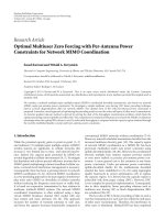
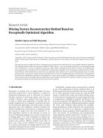
Figure 1: Optimal coefficients a
i
’s for the OSR.
terminate the sifting process. A commonly used criterion is
the sum of difference (SD):
SD
=
T

n=0


h
k−1
(n) − h
k
(n)



2
h
2
k
−1
(n)
. (2)
When the SD is smaller than a threshold, the first IMF c
1
(n)
is obtained, which is written as
r
1
(n) = x(n) −c
1
(n). (3)
Note that the residue r
1
(n) still contains some useful
information. We can therefore treat the residue as a new
signal and apply the above procedure to obtain
r
1
(n) − c
2
(n) = r
2
(n)
.
.

.
r
N−1
(n) − c
N
(n) = r
N
(n).
(4)
The whole procedure terminates when the residue r
N
(n)is
either a constant, a monotonic slope, or a function with
only one extremum. Combining the equations in (3)and(4)
yields the EMD of the original signal,
x(n)
=
N

i=1
c
i
(n)+r
N
(n). (5)
The result of the EMD produces N IMFs and a residue
signal. For convenience, we refer to c
i
(n) as the ith-order IMF.
By this convention, lower order IMFs capture fast oscillation

modes while higher order IMFs typically represent slow
oscillation modes. If we interpret the EMD as a time-scale
analysis method, lower-order IMFs and higher-order IMFs
correspond to the fine and coarse scales, respectively. The
residue itself can be regarded as the last IMF.
B. Weng and K. E. Barner 3
−150
−100
−50
0
50
100
150
200
250
b
ij
1
2
3
4
5
6
7
8
IMF index i
1
0.5
0
−0.5

−1
Sample index
j
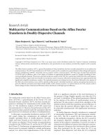
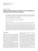
Figure 2: Optimal coefficients b
ij
’s for the BOSR.
−1
−0.5
0
0.5
1
1.5
2
b
r
ij
1
2
3
4
5
6
7
8
IMF index i
1
0.5
0
−0.5
−1

Sample index
j
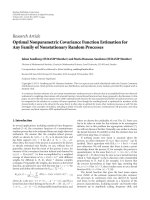
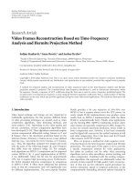
Figure 3: Optimal coefficients b
ij
’s for the RBOSR.
3. OPTIMAL SIGNAL RECONSTRUCTION USING EMD
The traditional empirical mode decomposition presented
in the previous section is a perfect reconstruction (PR)
decomposition as the sum of all IMFs yields the original
signal. Consider the related problem in which the objective is
to combine the IMFs in a fashion that approximates a signal
d(n) that is related to x(n). This problem is exemplified by
signal denoising application where x(n) is a noise-corrupted
version of d(n) and the aim is to reconstruct d(n)fromx(n).
The IMFs can be combined utilizing various methodologies
and under various objective functions designed to approxi-
mate d(n). We consider several such methods beginning with
a simple linear weighting,

d(n) =
N

i=1
a
i
c
i
(n), (6)
where the coefficient a
i

is the weight assigned to the ith IMF.
Note that, for convenience, the residue term is absorbed in
the summation as the last term c
N
(n). Also, the IMFs are
generated by decomposing x(n), which has some relationship
with the desired signal d(n). To optimize the a
i
coefficients,
we employ the mean square error (MSE),
J
1
= E

d(n) −

d(n)

2

=
E

d(n) −
N

i=1
a
i
c

i
(n)

2

.
(7)
The optimal coefficients can be determined by taking the
derivative of (7)withrespecttoa
i
and setting it to zero.
Therefore, we obtain
N

j=1
a
j
E

c
i
(n)c
j
(n)

=
E

d(n)c
i

(n)

,(8)
or equivalently,
N

i=1
R
ij
a
j
= p
i
, i = 1, , N (9)
by defining
p
i
= E

d(n)c
i
(n)

, R
ij
= E

c
i
(n)c

j
(n)

.
(10)
The above N equations can be written in a matrix form as
follows:
⎡
⎢
⎢
⎢
⎢
⎣
R
11
R
12
··· R
1N
R
21
R
22
··· R
2N
.
.
.
.
.

.
.
.
.
.
.
.
R
N1
R
N2
··· R
NN
⎤
⎥
⎥
⎥
⎥
⎦
⎡
⎢
⎢
⎢
⎢
⎣
a
1
a
2
.

.
.
a
N
⎤
⎥
⎥
⎥
⎥
⎦
=
⎡
⎢
⎢
⎢
⎢
⎣
p
1
p
2
.
.
.
p
N
⎤
⎥
⎥
⎥

⎥
⎦
, (11)
which can be compactly written as
R
1
a = p. (12)
The optimal coefficients are thus given by
a
∗
= R
−1
1
p. (13)
The dimension of the matrix R
1
is N × N. Since the
number of IMFs N is usually a small integer number, the
matrix inversion does not incur any numerical difficulties.
The minimum MSE can also be found by substituting (13)
into (7), which yields
J
1,min
= E

d(n) −
N

i=1
a

∗
i
c
i
(n)

2

=
σ
2
d
−p
T
R
−1
1
p,
(14)
where σ
2
d
= E{d
2
(n)} is the variance of the desired signal. In
practice, p
i
and R
ij
are estimated by sample average.

Many signals to which the EMD is applied are non-
stationary. Also matrix inversion may be too costly in
some situations. In such cases, an iterative gradient descent
adaptive approach can be utilized:
a
i
(n +1)= a
i
(n) − μ
∂J
1
∂a
i




a
i
=a
i
(n)
, (15)
4 EURASIP Journal on Advances in Signal Processing
1
0.8
0.6
0.4
0.2
0

−0.2
−0.4
−0.6
1000 1040 1080 1120 1160 1200
n
(a)
1
0.8
0.6
0.4
0.2
0
−0.2
−0.4
−0.6
1000 1040 1080 1120 1160 1200
n
Original
Linear filter
(b)
1
0.8
0.6
0.4
0.2
0
−0.2
−0.4
−0.6
1000 1040 1080 1120 1160 1200

n
Original
PAR-EMD
(c)
1
0.8
0.6
0.4
0.2
0
−0.2
−0.4
−0.6
1000 1040 1080 1120 1160 1200
n
Original
OSR
(d)
1
0.8
0.6
0.4
0.2
0
−0.2
−0.4
−0.6
1000 1040 1080 1120 1160 1200
n
Original

BOSR
(e)
1
0.8
0.6
0.4
0.2
0
−0.2
−0.4
−0.6
1000 1040 1080 1120 1160 1200
n
Original
RBOSR
(f)
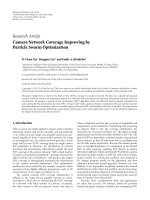
Figure 4: Denoising performance. Shown in dash lines are the original signal and the solid lines are denoised signals. (a) Noisy signal, (b)
linear Butterworth filter, (c) PAR-EMD, (d) OSR, (e) BOSR, (f) RBOSR.
B. Weng and K. E. Barner 5
−30
−25
−20
−15
−10
−5
0
−20 2
ω
B
1

(ω)
(a)
−20
−15
−10
−5
0
−20 2
ω
B
2
(ω)
(b)
−12
−10
−8
−6
−4
−2
0
−20 2
ω
B
3
(ω)
(c)
−40
−30
−20
−10

0
10
−20 2
ω
B
4
(ω)
(d)
−5
0
5
10
15
20
−20 2
ω
B
5
(ω)
(e)
−5
0
5
10
15
20
25
−20 2
ω
B

6
(ω)
(f)
−10
0
10
20
30
40
−20 2
ω
B
7
(ω)
(g)
−10
0
10
20
30
40
50
60
−20 2
ω
B
8
(ω)
(h)
Figure 5: Equivalent filter frequency responses for BOSR algorithm coefficients. Frequency responses of B

1
–B
8
are shown in dB values.
where μ is a positive number controlling the convergence
speed. By taking the gradient and using instantaneous
estimate for expectation, we obtain
∂J
1
∂a
i
=−2E

d(n) −
N

i=1
a
i
(n)c
i
(n)

c
i
(n)

=−
2E


e(n)c
i
(n)

≈−2e(n)c
i
(n).
(16)
Therefore, the weight update equation (15)canbewrittenas
a
i
(n +1)= a
i
(n)+2μe(n)c
i
(n), i = 1, , N. (17)
From the above formulation, it is clear that the OSR is
very similar to the Wiener filtering, which aims to estimate
a desired signal by passing a signal through a linear filter.
The main difference is that the OSR operates samples
in the EMD domain and weights samples according to
the IMF order while the Wiener filter applies filtering to
time domain signals directly and weights them temporally.
Two special cases of the OSR are remarked as follows. If
all the coefficients a
i
= 1, then it is equivalent to the
original perfect reconstruction EMD (PR-EMD). If some
coefficients are set to zero while others are set to one, it
reduces to the partial reconstruction EMD (PAR-EMD) used

in [8, 15]. Therefore, the OSR extends the capability of
the traditional EMD reconstruction and more importantly,
yields the optimal estimate of a given signal in the mean
square error sense.
4. BIDIRECTIONAL OPTIMAL SIGNAL
RECONSTRUCTION USING EMD
In the EMD, there are two directions in the resulting IMFs.
The first direction is the vertical direction denoted by the
IMF order i in (5). The vertical direction corresponds
to different scales. The other direction is the horizontal
direction represented by the time index n in (5). This
direction captures the time evolution of the signal. The
OSR proposed in the last section only uses the weighting
along the vertical direction. Therefore, it lacks degree of
freedom in the horizontal, or temporal direction. In some
circumstances, adjacent signal samples are correlated and
this factor must be considered when performing reconstruc-
tion.
A more flexible EMD reconstruction algorithm that
incorporates the signal correlation among samples in a
6 EURASIP Journal on Advances in Signal Processing
−30
−25
−20
−15
−10
−5
0
−20 2
ω

B
r
1
(ω)
(a)
−20
−15
−10
−5
0
−20 2
ω
B
r
2
(ω)
(b)
−14
−12
−10
−8
−6
−4
−2
0
−20 2
ω
B
r
3

(ω)
(c)
−35
−30
−25
−20
−15
−10
−5
0
−20 2
ω
B
r
4
(ω)
(d)
−25
−20
−15
−10
−5
0
−20 2
ω
B
r
5
(ω)
(e)

−50
−40
−30
−20
−10
0
−20 2
ω
B
r
6
(ω)
(f)
−15
−10
−5
0
5
10
−20 2
ω
B
r
7
(ω)
(g)
−12
−10
−8
−6

−4
−2
0
−20 2
ω
B
r
8
(ω)
(h)
Figure 6: Equivalent filter frequency responses for RBOSR algorithm coefficients. Frequency responses of B
1
–B
8
are shown in dB values.
temporal window is described as follows. For a specific
time n, a temporal window of size 2M +1ischosen
with the current sample being the center of the win-
dow. Weighting is concurrently employed to account for
the relations between IMFs. Consequently, 2D weight-
ing coefficients b
ij
are utilized to yield the estimated
signal

d(n) =
N

i=1
M


j=−M
b
ij
c
i
(n − j), (18)
where M is the half window length. This formulation
takes both vertical and horizontal directions into con-
sideration and is thus referred to as the bidirectional
optimal signal reconstruction (BOSR). From (18), the
bidirectional weighting can be interpreted as follows. The
ith IMF c
i
(n) is passed through a FIR filter b
ij
of length
2M + 1. Thus we have a filter bank consisting of N FIR
filters, each of which is applied to an individual IMF.
The final output is the summation of all filter outputs.
Compared to the OSR, the BOSR makes use of the cor-
relation between the samples. However, the cost paid for
the gained degrees of freedom is increased computational
complexity.
Similar to the OSR, the optimization criterion chosen
here is the mean square error
J
2
= E


d(n) −
N

i=1
M

j=−M
b
ij
c
i
(n − j)

2

. (19)
Differentiating, with respect to the coefficient b
ij
and setting
it to zero, yields
N

k=1
M

l=−M
b
kl
R
2

(k,i; l, j) = p
2
(i, j),
i
= 1, ,N, j =−M, , M,
(20)
wherewedefine
R
2
(k,i; l, j) = E

c
k
(n − l)c
i
(n − j)

, (21)
p
2
(i, j) = E

d(n)c
i
(n − j)

. (22)
It can be seen that the correlation in (21) is bidirectional
with a quadruple index representing both IMF order and
B. Weng and K. E. Barner 7

temporal directions. There are altogether (2M +1)N equa-
tions in (20) and if we rearrange the R
2
(k,i; l, j)andp
2
(i, j)
according to the lexicographic order, (20) can be put into the
following matrix equation:
⎡
⎢
⎢
⎢
⎢
⎣
R
2
(1, 1; −M,−M) R
2
(1, 1; −M +1,−M) ··· R
2
(N,1;M, −M)
R
2
(1, 1; −M,−M +1) R
2
(1, 1; −M +1,−M +1) ··· R
2
(N,1;M, −M +1)
.
.

.
.
.
.
.
.
.
.
.
.
R
2
(1, N;−M, M) R
2
(1, N;−M +1,M) ··· R
2
(N, N; M, M)
⎤
⎥
⎥
⎥
⎥
⎦
⎡
⎢
⎢
⎢
⎢
⎣
b

1,−M
b
1,−M+1
.
.
.
b
N,M
⎤
⎥
⎥
⎥
⎥
⎦
=
⎡
⎢
⎢
⎢
⎢
⎣
p
2
(1, −M)
p
2
(1, −M +1)
.
.
.

p
2
(N, M)
⎤
⎥
⎥
⎥
⎥
⎦
. (23)
Equation (23) can be compactly written as
R
2
b = p
2
, (24)
from which the optimal solution b
∗
is given by
b
∗
= R
−1
2
p
2
. (25)
The dimension of the matrix R
2
is (2M +1)N ×(2M +1)N,

so the computational complexity due to matrix inversion is
increased from O(N
3
) for the OSR algorithm to O((2M +
1)
3
N
3
). However, since the BOSR performs weighting in IMF
order and temporal directions, it can better capture signal
correlations. The elements of the matrix R
2
and the vector p
can be estimated by sample averages. As in the OSR case, an
adaptive approach can be utilized. After some derivation, we
obtain the weight update equation for BOSR:
b
ij
(n +1)= b
ij
(n)+2μe(n)c
i
(n − j),
i
= 1, ,N, j =−M , M.
(26)
In the BOSR, the memory length M needs to be chosen.
More samples in the window will improve the performance
as more signal memories are taken into consideration to
account for the temporal correlation. However, the perfor-

mance gain is no longer substantial when M is increased
to a certain number. As such, we can set up an objective
function similar to Akaike information criterion (AIC) to
determine the optimal memory length M [16]. This process
is analogous to choosing model order in the statistical
modeling.
4.1. Regularized bidirectional optimal
signal reconstruction using EMD
Although the BOSR considers the time domain correlations
between samples, a problem arises in calculating the optimal
coefficients b
∗
by (25), as the matrix R
2
is sometimes ill
conditioned.
To s e e w h y R
2
is sometimes ill conditioned, let R
2
=
E{c(n)c
T
(n)} where
c(n)
=

c
1
(n + M), , c

1
(n − M), c
2
(n + M), ,
c
2
(n − M), ,c
N
(n + M), , c
N
(n − M)

T
.
(27)
Also denote R
2
(:, k) as the kth column of the matrix R
2
.It
can be shown that
R
2
(:, k) = E

c(n)c
i
(n − j)

, (28)

where k
= (i − 1) × (2M +1)+j + M +1fori = 1, , N,
j
=−M, , M. Note that when the IMF order i is large,
c
i
(n) tends to have fewer oscillations and thus fewer changes
between consecutive samples. The extreme case is a nearly
constant residue for the last IMF c
N
(n). Thus, c
i
(n)becomes
smoother when the order i becomes large. Due to this fact,
c
i
(n − j)andc
i
(n − j + 1) are very similar for large i.
Consequently, the two columns R
2
(:, k)andR
2
(:, k +1)are
also very similar, which results in R
2
being ill conditioned.
To alleviate the potential ill-condition problem of the
BOSR, we propose a regularized version of the BOSR
(RBOSR). The original objective function J

2
does not
place any constraints on the b
ij
coefficients. We add some
regularizing conditions on b
ij
by restricting their values to
be in the range
−U ≤ b
ij
≤ U. This condition implies that
the magnitudes of the coefficients are bounded by a constant
U.
The original problem is thus changed into the following
constrained optimization problem:
minimize J
2
= E

d(n) −
N

i=1
M

j=−M
b
ij
c

i
(n − j)

2

subject to − U ≤b
ij
≤ U, ∀1≤i≤N, −M ≤j ≤M.
(29)
To solve the above constrained optimization problem, we
can invoke the Kuhn-Tucker condition [17], which gives a
necessary condition for the optimal solution. The Lagrangian
of the minimization problem can be written as
L

b
ij
, μ
ij
, λ
ij

=
J
2

b
ij

+

N

i=1
M

j=−M
μ
ij

−
b
ij
−U

+
N

i=1
M

j=−M
λ
ij

b
ij
−U

.
(30)

Applying the Kuhn-Tucker condition yields the following
equations:
∇L

b
ij
, μ
ij
, λ
ij

=
∂J
2
∂b
ij
−μ
ij
+ λ
ij
= 0,
μ
ij

−
b
ij
−U

=

0,
λ
ij

b
ij
−U

= 0,
μ
ij
≥ 0,
λ
ij
≥ 0.
(31)
8 EURASIP Journal on Advances in Signal Processing
10
−4
10
−3
10
−2
10
−1
MSE
0 5 10 15 20 25
SNR (dB)
Linear filter
PAR-EMD

OSR
BOSR
RBOSR
Figure 7: MSE versus SNR for three different denoising algorithms.
Iterative algorithms for general nonlinear optimization, such
as the interior point method, can be utilized to find the
optimal solution to the above problem [17]. A fundamental
point of note is that the solution is guaranteed to be globally
optimal since both the objective function and constraints are
convex functions.
An alternative approach to solve the constrained mini-
mization problem is to view it as a quadratic programming
problem. The objective function can be rewritten as
J
2
= E

d(n) −
N

i=1
M

j=−M
b
ij
c
i
(n − j)


2

=
E

d
2
(n)

−
2b
T
p
2
+ b
T
R
2
b,
(32)
where b, p
2
, R
2
are defined as in (24), and c(n) is the vector
in (27). The optimization problem can thus be restated as a
standard quadratic programming problem:
minimize J

2

= b
T
R
2
b − 2p
T
2
b
subject to
−U  b  U,
(33)
where the symbol  denotes component-wise less than or
equal to for vectors. Since the objective function is convex
and the inequality constraints are simple bounds, a faster
conjugate gradient search for quadratic programming can be
performed to find the optimal solution [17].
5. APPLICATIONS
Having established the OSR and BOSR algorithms, we apply
them to various applications. Two examples are given. The
first application considered is signal denoising, where sim-
ulated random signals are used. In the second example, the
proposed algorithms are applied to real biomedical signals
10
−4
10
−3
10
−2
10
−1

MSE
0 5 10 15 20 25
SNR (dB)
M
= 1
M
= 2
M
= 3
M
= 4
M
= 5
(a)
10
−2.55
10
−2.54
10
−2.53
10
−2.52
10
−2.51
MSE
14.94 14.96 14.98 15 15.02 15.04 15.06 15.08
SNR (dB)
M
= 1
M

= 2
M
= 3
M
= 4
M
= 5
(b)
Figure 8: Performances for different memory length. (a) Large-
scale view, (b) zoomed-in view.
to remove ECG interferences from EEG recording. The
following example illustrates the denoising using the OSR,
BOSR, and RBOSR algorithms and compares them with the
linear lowpass filtering and the partial reconstruction EMD
(PAR-EMD) in [15]. The PAR-EMD method is based on the
IMF signal energy and the reconstructed signal is given by
the partial summation of those IMFs whose energy exceeds
an established threshold.
Example 1. The original signal in this example is a bilinear
signal model:
x(n)
= 0.5x(n −1) + 0.6x(n −1)v(n −1) + v(n), (34)
B. Weng and K. E. Barner 9
Table 1: Optimal coefficients of the OSR algorithm.
IMF order i 12345678
a
∗
i
0.2859 0.5150 0.8496 0.8833 0.9710 0.9609 0.9639 0.9653
Table 2: Optimal coefficients of the BOSR algorithm (M = 1).

b
∗
ij
IMF order i
123 4 5 6 7 8
−1 0.2219 0.3843 0.2322 0.5301 −1.4488 −3.0298 8.7950 −123.9047
0 0.4654 0.3261 0.2439
−0.1592 3.6319 7.1100 −19.3460 246.7700
1 0.1899 0.2149 0.5048 0.5612
−1.2579 −3.1527 11.6191 −121.9207
where v(n) is white noise with variance equal to 0.01. Bilinear
signal model is a type of nonlinear signal model. Additive
Laplacian noise with variance 0.0092 is added to the signal
to attain a SNR
= 10 dB, where SNR is defined as the
ratio of signal power and noise variance. The total signal
length is 2000 and the first 1000 samples are used as the
training signal d(n) to estimate the optimal OSR, BOSR, and
RBOSR coefficients. Once these coefficients are determined,
the remaining samples are tested for denosing. The denoised
signal is obtained by substituting the optimal coefficients into
the reconstruction formulae (6)and(18). In the following,
the denoising performance is evaluated by the mean square
error calculated as
MSE
=
1
L
2
−L

1
+1
L
2

n=L
1

x
o
(n) − x(n)

2
, (35)
where L
1
and L
2
are starting and ending indices of testing
samples, and x
o
(n)andx(n) are original noise-free and
denoised signals, respectively.
In the following, the signal memory M in the BOSR
is chosen to be 1. Eight IMFs are obtained after the EMD
decomposition. Hence, the total number of a
i
coefficients
is 8 and the total number of b
ij

coefficients is 24. In the
RBOSR algorithm, the regularizing bound U is chosen to be
10. The optimal coefficients a
∗
i
and b
∗
ij
obtained by the OSR,
BOSR, RBOSR are listed in Tables 1, 2,and3,respectively.
These coefficients are also graphically represented by Figures
1, 2,and3. It can be observed that the first several weighting
coefficients for the OSR are relatively small. As the IMF order
increases, the a
i
coefficients also increase to some values close
to one. This can be seen as a generalization of the PAR-EMD
in which binary selection on the IMFs is replaced by linear
weighting of the IMFs. The result is also in agreement with
that of the PAR-EMD where it is found that the lower-order
IMFs contain more noise components than the higher-order
IMFs. Consequently, lower-order IMFs should be assigned
small weights in denoising. When comparing the optimal
b
ij
coefficients obtained by the BOSR and RBOSR, we see
that the BOSR yields coefficients that differ in magnitude
on the order of thousands (see Tab le 2 and Figure 2), while
the optimal coefficients obtained by the RBOSR are closer
to each other (see Ta bl e 3 and Figure 3). Therefore, the

regularization process mitigates the numerical instability of
the original BOSR algorithm.
−10
10
(μV)
16 18 20 22 24 26 28 30
Time (s)
(a)
−10
10
(μV)
16 18 20 22 24 26 28 30
Time (s)
(b)
−10
10
(μV)
16 18 20 22 24 26 28 30
Time (s)
(c)
−10
10
(μV)
16 18 20 22 24 26 28 30
Time (s)
(d)
−10
10
(μV)
16 18 20 22 24 26 28 30

Time (s)
(e)
−10
10
(μV)
16 18 20 22 24 26 28 30
Time (s)
(f)
−10
10
(μV)
16 18 20 22 24 26 28 30
Time (s)
(g)
Figure 9: ECG interference removal in EEG. (a) Original EEG,
(b) EEG containing ECG interferences, (c) OSR (MSE
= 4.1883),
(d) adaptive OSR (MSE
= 3.3599), (e) BOSR (MSE = 2.7189), (f)
adaptive BOSR (MSE
= 2.3354), (g) RBOSR (MSE = 2.0432).
10 EURASIP Journal on Advances in Signal Processing
Table 3: Optimal coefficients of the regularized BOSR algorithm (M = 1).
b
∗
ij
IMF order i
123456 7 8
−1 0.2235 0.3774 0.2196 0.3947 0.1248 0.3133 −0.8960 0.0719
0 0.4651 0.3275 0.2643 0.1128 0.5437 0.3387 0.3509 0.3213

1 0.1891 0.2102 0.4897 0.4160 0.3245 0.3193 1.5481 0.5592
The denoising results are shown in Figure 4 where we
also show the results of the Butterworth lowpass filtering
and the PAR-EMD algorithm. The noisy signal is shown
in Figure 4(a) in which testing samples from 1000–1200
are shown. Figures 4(b), 4(c), 4(d), 4(e),and4(f) show
the denoised signals reconstructed by the linear filter, PAR-
EMD, OSR, BOSR, and RBOSR, respectively, and compare
the resulting signals with the original signal. It can be seen
that the OSR, BOSR, and RBOSR produce a signal closer to
the original signal than the other two methods. However,
the BOSR performs slightly better than the OSR since
the residual error is smaller. The reason for the improved
performance is that the BOSR takes the signal correlation
into account. Furthermore, the performances of the BOSR
and RBOSR are very close. This shows that even though
the coefficients of the BOSR are much more dispersed than
those of RBOSR, the BOSR performance does not suffer from
this. Measured quantitatively by the MSE from (35), these
algorithms yield MSE of 0.0193 for linear filter, 0.01 for the
PAR-EMD, 0.0063 for the OSR, 0.0046 for the BOSR, and
0.0046 for the RBOSR.
We re ma rke d i n Section 4 that the bidirectional b
ij
coefficients act as a FIR filter in the time domain for the ith
IMF. Therefore, it is interesting to investigate the behavior of
these filters as the order of IMF changes. Starting from the
first IMF, we plot the frequency responses of the filters used
in the BOSR algorithm in Figure 5. It can be seen that the first
filter B

1
(ω) applied to IMF 1 exhibits lowpass characteristics.
As the IMF order increases, the filters first become bandpass
filters and then more highpass-like filters. In the denoising
application, the first IMF contains strong noise components.
So the filter tries to filter the noise out and leaves only
lowpass signal components. For the mid-order IMFs, noise
components are mainly located in certain frequency bands,
which tunes the filter to be bandpass. For high-order IMFs,
the filter gain is high and the DC frequency range is nearly
kept unchanged (0 dB). The BOSR is equivalent to filtering
the signal by N different filters in N different IMFs. This
will not be possible if we simply use the partial summation
of IMFs. The frequency responses of the filters used in the
RBOSR are also shown in Figure 6 with a different behavior
observed. These filters are either of lowpass or bandpass
type and no highpass characteristics are exhibited. Also, the
filter gains for RBOSR are generally smaller than those of
BOSR,whichisaresultofcoefficient regularization in the
optimization process.
A more thorough study using a wide range of different
realizations of stochastic signals is carried out by Monte
Carlo simulation. Figure 7 shows the MSE versus SNR for
the five algorithms: linear filtering, PAR-EMD, OSR, BOSR,
and RBOSR. At each SNR, 500 runs are performed to obtain
an averaged MSE as shown in the figure. We see that the
OSR and BOSR algorithms outperform the linear filtering
and PAR-EMD over the entire SNR range. The performances
of the BOSR and RBOSR are better than that of the OSR,
as expected. The BOSR performs slightly better than the

RBOSR even though its coefficients are less regular.
To investigate the effects of the memory length M on the
BOSR performance, five different values of M are chosen
(M
= 1, 2, 3,4, 5). Monte Carlo simulation is carried out
to compare the performances of the BOSR for different
Ms. From Figure 8(a), using larger M does not significantly
improve the performance as we see those curves are getting
closer to each other as M increases. A zoomed-in view
around SNR
= 15 dB in Figure 8(b) more clearly shows that
larger M yields lower MSE, though this difference is not
easily distinguishable from the larger scale plot. It is therefore
advised to choose a small M instead of large M in the BOSR
since small M can do as good a job as large M but with less
complexity.
Example 2. Electroencephalogram (EEG) is widely used
as an important diagnostic tool for neurological disorder.
Cardiac pulse interference is one of the sources that affect the
EEG recording [18]. The EMD method is especially useful
for nonlinear and nonstationary biomedical signals [19–22].
The optimal reconstruction algorithms based on EMD are
therefore used to remove the ECG interferences from EEG
recording.
Real EEG and ECG recordings are obtained from a 37-
year-old woman at Alfred I., DuPont Hospital for Children
in Wilmington, Delaware. The signals are sampled at 128 Hz.
The EEG signal with ECG interferences is obtained by adding
attenuated ECG component to EEG, that is, x(t)
= x

e
(t)+
αx
c
(t), where x
e
(t) is the EEG, x
c
(t) is the ECG, and α = 0.6
reflects the attenuation in the pathways. The total duration
of recording is about 29 minutes and we select the first
2000 samples (0–15.625 seconds) as the training samples and
the next 2000 samples (15.625–31.25 seconds) as the testing
samples. The original EEG and the EEG containing ECG
interferences are shown in Figures 9(a) and 9(b),respectively.
It is clear that the spikes due to the QRS complex of ECG
is prominent in EEG. The spectra of ECG and EEG are
overlapped because the bandwidth for ECG monitoring is
0.5–50 Hz, while the frequency bands of EEG range from 0.5–
13 Hz and above [23]. Therefore, simple filtering techniques
cannot be used to separate EEG from ECG interferences.
The three optimal reconstruction methods, OSR, BOSR, and
B. Weng and K. E. Barner 11
RBOSR, together with their adaptive versions, are applied to
the ECG contaminated EEG signal. The memory length M
is set to 1 for both BOSR and RBOSR and the bound U
for RBOSR is chosen to be 10. The reconstructed samples
are shown in Figures 9(c), 9(d), 9(e), 9(f),and9(g).The
resulting signal of the OSR still has some residual spikes. Both
BOSR and RBOSR yield signal waveforms that are closer

to the original EEG. However, there is a baseline wander
in the initial stage of the BOSR result while this baseline
wander does not exist in the RBOSR result. Adaptive modes
of the OSR and BOSR are used and the results are shown
in Figures 9(d) and 9(f), respectively. From these figures, all
these optimal reconstruction methods are able to remove the
ECG interferences from EEG to some extent. But the BOSR
and RBOSR are better than the OSR, which agrees with the
first example. In terms of MSE, the OSR has MSE
= 4.1883
while the BOSR and RBOSR achieve MSE of 2.7189 and
2.0432, respectively. The adaptive modes of OSR and BOSR
yield MSE of 3.3599 and 2.3354, thus slightly improve the
original algorithms.
6. CONCLUSION
The empirical mode decomposition is a tool for analyzing
nonlinear and nonstationary signals. Conventional EMD,
however, does not impose on optimality conditions for
reconstruction from IMFs. In this paper, several improved
versions of EMD signal reconstruction that are optimal in the
minimum mean square error sense are proposed. The first
algorithm OSR estimates a given signal by linear weighting
of the IMFs. The coefficients are determined by solving a
linear set of equations. To consider the temporal structure
of a signal, BOSR is then proposed. The weighting of the
BOSR is carried out not only in the IMF order direction, but
also in the temporal direction. It is able to compensate for
the time correlation between adjacent samples. The proposed
algorithms are applied to signal denoising problem, where
both the OSR and BOSR have better performance than

the traditional partial reconstruction EMD. These methods
are also applied to real biomedical signals where ECG
interferences are removed from EEG recordings. The optimal
EMD reconstruction methods proposed in this paper give
some new insight to this promising signal analysis tool.
REFERENCES
[1] N. E. Huang, Z. Shen, S. R. Long, et al., “The empirical
mode decomposition and hilbert spectrum for nonlinear and
nonstationary time series analysis,” Proceedings of the Royal
Society A, vol. 454, no. 1971, pp. 903–995, 1998.
[2] P. Flandrin, G. Rilling, and P. Gonc¸alv
´
es, “Empirical mode
decomposition as a filter bank,” IEEE Signal Processing Letters,
vol. 11, no. 2, part 1, pp. 112–114, 2004.
[3] P. Flandrin and P. Gonc¸alv
´
es, “Empirical mode decomposition
as a data-driven wavelet-like expansions,” International Jour-
nal of Wavelets, Multiresolution and Information Processing,
vol. 2, no. 4, pp. 477–496, 2004.
[4] K. Coughlin and K. K. Tung, “Eleven-year solar cycle signal
throughout the lower atmosphere,” Journal of Geophysical
Research, vol. 109, no. D21, p. D21105, 2004.
[5]J.C.Nunes,S.Guyot,andE.Del
´
echelle, “Texture analysis
based on local analysis of the bidimensional empirical mode
decomposition,” Machine Vision and Applications, vol. 16, no.
3, pp. 177–188, 2005.

[6] D. Pines and L. Salvino, “Structural health monitoring
using empirical mode decomposition and the Hilbert phase,”
Journal of Sound and Vibration, vol. 294, no. 1-2, pp. 97–124,
2006.
[7] W. Huang, Z. Shen, N. E. Huang, and Y. C. Fung, “Engineering
analysis of biological variables: an example of blood pressure
over 1 day,” Proceedings of the National Academy of Sciences
of the United States of America, vol. 95, no. 9, pp. 4816–4821,
1998.
[8] H. Liang, Q H. Lin, and J. D. Z. Chen, “Application of the
empirical mode decomposition to the analysis of esophageal
manometric data in gastroesophageal reflux disease,” IEEE
Transactions on Biomedical Engineering, vol. 52, no. 10, pp.
1692–1701, 2005.
[9] B. Weng, M. Blanco-Velasco, and K. E. Barner, “ECG
denoising based on the empirical mode decomposition,” in
Proceedings of the 28th Annual International Conference of IEEE
Engineering in Medicine and Biology Society (EMBS ’06),pp.1–
4, New York, NY, USA, August-September 2006.
[10] J. C. Nunes, Y. Bouaoune, E. Delechelle, O. Niang, and Ph.
Bunel, “Image analysis by bidimensional empirical mode
decomposition,” Image and Vision Computing, vol. 21, no. 12,
pp. 1019–1026, 2003.
[11] R. Balocchi, D. Menicucci, E. Santarcangelo, et al., “Deriving
the respiratory sinus arrhythmia from the heartbeat time
series using empirical mode decomposition,” Chaos, Solitons
&Fractals, vol. 20, no. 1, pp. 171–177, 2004.
[12] N. Huang and N. O. Attoh-Okine, The Hilbert-Huang Trans-
form in Engineering, CRC Press, Boca Raton, Fla, USA, 2005.
[13] B. Weng, M. Blanco-Velasco, and K. E. Barner, “Baseline wan-

der correction in ECG by the empirical mode decomposition,”
in Proceedings of the 32nd Annual Northeast Bioengineering
Conference (NEBC ’06), pp. 135–136, Easton, Pa, USA, April
2006.
[14] E. Del
´
echelle, J. Lemoine, and O. Niang, “Empirical mode
decomposition: an analytical approach for sifting process,”
IEEE Signal Processing Letters, vol. 12, no. 11, pp. 764–767,
2005.
[15] P. Flandrin, P. Gonc¸alv
´
es, and G. Rilling, “Detrending and
denoising with empirical mode decomposition,” in Pro-
ceedings of the 12th European Signal Processing Conference
(EUSIPCO ’04), Viena, Austria, September 2004.
[16] H. Akaike, “A new look at the statistical model identification,”
IEEE Transactions on Automatic Control,vol.19,no.6,pp.
716–723, 1974.
[17] D. G. Luenberger, Introduction to Linear and Nonlinear
Programming, Addison-Wesley, Reading, Mass, USA, 1973.
[18] J. Sijbersa, J. Van Audekerke, M. Verhoye, A. Van der Linden,
and D. Van Dyck, “Reduction of ECG and gradient related
artifacts in simultaneously recorded human EEG/MRI data,”
Magnetic Resonance Imaging, vol. 18, no. 7, pp. 881–886, 2000.
[19] M. Blanco-Velasco, B. Weng, and K. E. Barner, “A new ECG
enhancement algorithm for stress ECG tests,” in Proceedings
of IEEE International Conference on Computer in C ardiology
(CIC ’06), pp. 917–920, Valencia, Spain, September 2006.
[20] B. Weng, G. Xuan, J. Kolodzey, and K. E. Barner, “Empirical

mode decomposition as a tool for DNA sequence analysis
from terahertz spectroscopy measurements,” in Proceedings of
IEEE International Workshop on Genomic Signal Processing and
Statistics (GENSIPS ’06), pp. 63–64, College Station, Tex, USA,
May 2006.
12 EURASIP Journal on Advances in Signal Processing
[21] J. Dauwels, T. M. Rutkowski, F. Vialatte, and A. Cichocki,
“On the synchrony of empirical mode decompositions with
application to electroencephalography,” in Pro ceedings of
IEEE International Conference on Acoustics, Speech and Sig nal
Processing (ICASSP ’08), pp. 473–476, Las Vegas, Nev, USA,
March 2008.
[22] M. Blanco-Velasco, B. Weng, and K. E. Barner, “ECG signal
denoising and baseline wander correction based on the
empirical mode decomposition,” Computers in Biology and
Medicine, vol. 38, no. 1, pp. 1–13, 2008.
[23] R. M. Rangayyan, Biomedical Signal Analysis: A Case-Study
Approach, IEEE Press, New York, NY, USA, 2002.