Báo cáo hóa học: " Research Article A Multiuser MIMO Transmit Beamformer Based on the Statistics of the Signal-to-Leakage Ratio" doc

Hindawi Publishing Corporation
EURASIP Journal on Wireless Communications and Networking
Volume 2009, Article ID 679430, 10 pages
doi:10.1155/2009/679430
Research Article
A Multiuser MIMO Transmit Beamformer Based on the Statistics
of the Signal-to-Leakage Ratio
Batu K. Chalise and Luc Vandendorpe
Communication and Remote Sensing Laboratory, Universit
´
e Catholique de Louvain, Place du Levant 2,
1348 Louvain-la-Neuve, Belgium
Correspondence should be addressed to Batu K. Chalise,
Received 23 February 2009; Accepted 3 June 2009
Recommended by Alex Gershman
A multiuser multiple-input multiple-output (MIMO) downlink communication system is analyzed in a Rayleigh fading
environment. The approximate closed-form expressions for the probability density function (PDF) of the signal-to-leakage ratio
(SLR), its average, and the outage probability have been derived in terms of the transmit beamformer weight vector. With the
help of some conservative derivations, it has been shown that the transmit beamformer which maximizes the average SLR also
minimizes the outage probability of the SLR. Computer simulations are carried out to compare the theoretical and simulation
results for the channels whose spatial correlations are modeled with different methods.
Copyright © 2009 B. K. Chalise and L. Vandendorpe. This is an open access article distributed under the Creative Commons
Attribution License, which permits unrestricted use, distribution, and reproduction in any medium, provided the original work is
properly cited.
1. Introduction
The capacity of a wireless cellular system is limited by
the mutual interference among simultaneous users. Using
multiple antenna systems, and in particular, the adaptive
beamforming, this problem can be minimized, and the
system capacity can be improved. In recent years, the
optimum downlink beamforming problem (including power

control) has been extensively studied in [1–3] where the
signal-to-interference-plus-noise ratio (SINR) is used as
a quality of service (QoS) criterion. After it has been
found that the multiple-input multiple-output (MIMO)
techniques significantly enhance the performance of wireless
communication systems [4, 5], the joint optimization of
the transmit and receive beamformers [6] has also been
investigated for MIMO systems. Motivated by the fact
that the optimum transmit beamformers [1–3] and the
joint optimum transmit-receive beamformers [6]canbe
obtained only iteratively due to the coupled nature of
the corresponding optimization problems, recently, the
concept of leakage and subsequently the signal-to-leakage-
plus-noise ratio (SLNR) as a figure of merit have been
introducedin[7, 8]. (Note that SLNR as a performance
criterion has been considered in [9–11] for multiple-
input-single-output (MISO) systems.) Although the latter
approach only gives suboptimum solutions, it leads to a
decoupled optimization problem and admits closed-form
solutions for downlink beamforming in multiuser MIMO
systems.
While investigating multiuser systems from a system
level perspective, in many cases, the outage probability has
also been widely used as a QoS parameter. The closed-
form expressions of the outage probability with equal gain
and optimum combining have been derived in [12, 13],
respectively, in a flat-fading Rayleigh environment with
cochannel interference. The latter work has been extended
in [14] to a Rician-Rayleigh environment where the desired
signal and interferers are subject to Rician and Rayleigh

fading, respectively. However, in all of the above-mentioned
papers, investigations have been limited to the derivations
of the outage probability expressions for specific types of
receivers. The outage probability of the signal-to-interference
ratio is used to formulate the optimum power control
problem for interference limited wireless systems in [15, 16]
where the total transmit power is minimized subject to
outage probability constraints. However, both of the these
works [15, 16] are limited to systems with single antenna at
transmitters and receivers.
2 EURASIP Journal on Wireless Communications and Networking
s
1
w
1
s
K
w
K
x
M
H
1
H
K
N
1
N
K
User1

UserK
s
1
s
K
Base station Channel
.
.
.
.
.
.
.
.
.
.
.
.
.
.
.
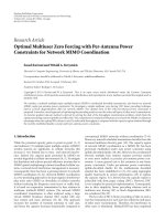
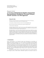
Figure 1: Multiuser MIMO downlink beamforming.
In this paper, we consider the downlink of a multiuser
MIMO wireless communication system in a Rayleigh fading
environment. The base station (BS) communicates with
several cochannel users in the same time and frequency slots.
In our method, we use the average signal-to-leakage ratio
(SLR) and the outage probability of SLR as performance
metrics which are based on the concept of leakage power
[7, 8]. In particular, the novelty of our work lies on the

facts that we first derive an approximation of the statistical
distribution of SLR [7] for each cochannel user of the MIMO
system in terms of transmit beamforming weight vector.
Second, the approximate closed-form expression for the
outage probability of SLR is derived. Then, we obtain the
solution for the transmit beamformer that minimizes the
aforementioned outage probability. According to our best
source of knowledge, this approach has not been previously
considered for the multiuser MIMO downlink beamforming.
With some conservative derivations, we also demonstrate
that the beamformer which minimizes the outage probability
is same as the one which maximizes the average SLR.
Note that similar conclusion has been made in [17]where
the downlink beamforming for multiuser MISO systems
is analyzed using the SINR and its outage probability as
the performance criteria. In contrast to [7], we consider
that the BS has only the knowledge of the second-order
statistics such as the covariance matrix of the downlink user-
channels. The motivation behind this assumption is that
the knowledge of instantaneous channel information can be
available at the BS only through the feedback from users.
The drawbacks of the feedback approach are the reduction
of the system capacity because of the frequent channel usage
required for the transmission of the feedback information
from users to the BS, and inherent time delays, errors, and
extra costs associated with such a feedback. Furthermore,
if the channel varies rapidly, it is not reasonable to acquire
the instantaneous feedback at the transmitter, because the
optimal transmitter designed on the basis of previously
acquired information becomes outdated quickly (see [18]

and the references therein). Thus, we consider that no full-
rate feedback information is available at the BS.
The remainder of this paper is organized as follows.
The system model is presented in Section 2. The probability
density function (PDF) of SLR, its mean, and the outage
probability of SLR are derived in terms of the beamformer
weight vector in Section 3.InSection 4, the transmit beam-
former which maximizes the average SLR and minimizes
the outage probability is obtained. In Section 5,analytical
and numerical results are compared. Finally, conclusions are
drawn in Section 6.
Notational conventions. Upper (lower) bold face letters will
be used for matrices (vectors); (
·)
H
,E{·}, I
n
, ·,tr(·),
and C
M×M
denote the Hermitian transpose, mathematical
expectation, n
× n identity matrix, Euclidean norm, trace
operator, and the space of M
× M matrices with complex
entries, respectively.
2. System Model
Consider a downlink multiuser scenario with a multi-
antenna BS of M sensors communicating with K
multi-antenna users. (If there are multiple BSs and they have

also the channel information of users assigned to other BSs,
the SLR-based method needs to be modified in such a way
that each BS takes into account the power leaked by it to the
users of other BSs. The necessary modifications, in our case,
can be done with some straightforward steps.) The block
diagram is shown in Figure 1. The signal transmitted by the
BS is given by
x
=
K

k=1
w
k
s
k
∈ C
M×1
,(1)
where s
k
and w
k
∈ C
M×1
are, respectively, the signal stream
and the transmit beamformer weight vector for kth user.
It is assumed that E
{s
k

}=0andE{|s
k
|
2
}=1fork =
1, , K.(We consider equal power allocations to all users.
Note that power control can be included in the design
of beamformers by using a two-step approach, that is, by
optimizing the beamformers first and then the powers or
vice-versa [1, 2].) Moreover, following the spirit of [7], we
consider that the beamformer weights are normalized, that
is,
w
k

2
= 1. Let N
i
denote the number of receive antennas
at ith user. The signal vector received by ith user is
y
i
=


G
i
H
i
x + n

i

∈
C
N
i
×1
,(2)
where G
i
is a constant that includes the effect of distance-
dependent path loss factor and the distance-independent
mean-channel power gain, H
i
∈ C
N
i
×M
is the spatially
correlated MIMO channel matrix, and n
i
∈ C
N
i
×1
denotes
the additive noise. It is assumed that each user is surrounded
by a large number of scatterers whereas the BS, which
is generally located at larger heights from the ground
level, does not observe rich scattering. In this scenario,

the MIMO channel as seen from the user/BS is spatially
uncorrelated/correlated. Thus, the ith MIMO channel can
be given by replacing the receive correlation matrix with
an identity matrix in the famous Kronecker-model [19]
which turns into the following form: H
i
= H
i
w
Σ
1/2
i
,where
the entries of H
i
w
∈ C
N
i
×M
are assumed to be zero-mean
EURASIP Journal on Wireless Communications and Networking 3
circularly symmetric complex Gaussian (ZMCSCG) random
variables with unit variance such that E
{tr((H
i
w
)
H
H

i
w
)}=
N
i
M,andΣ
i
∈ C
M×M
represents the spatial correlation
matrix at the BS corresponding to the ith user channel. It
is important to emphasize here that the derivations for the
SLR mean and SLR ouatge probability can be easily extended
to double-sided correlated MIMO channels (including the
user side correlation), and thus, our main results are also
valid for such MIMO channels. Note that Σ
i
are symmetric
positive semidefinite matrices and are a function of the
antenna spacing, average direction of arrival of the scattered
signal from ith user, and the corresponding angular spread
[20]. We invite our readers to have a look at [20] and the
references therein for determining Σ
i
. Furthermore, without
loss of generality, the elements of n
i
in (2) are considered to
be ZMCSCG with the variance σ
2

i
, that is, n
i
∼ N
C
(0, I
N
i
σ
2
i
),
where I
N
i
denotes N
i
× N
i
identity matrix. Inserting (1) into
(2) and applying the statistical expectation over signal and
noise realizations, the SLNR for ith user can be expressed as
[7]
SLNR
i
=
G
i
H
i

w
i

2
N
i
σ
2
i
+

K
k=1,k
/
=i
G
k
H
k
w
i

2
. (3)
Note that, here, G
i
H
i
w
i


2
is the power of the desired signal
for user i whereas G
k
H
k
w
i

2
is the power of interference
that is caused by user i on the signal received by some
other user k. The leakage for user i is thus the total
power leaked from this user to all other users which is

K
k
=1,k
/
=i
G
k
H
k
w
i

2
. The objective of beamformer is to

make G
i
H
i
w
i

2
as large as possible when compared to
the leakage power

K
k=1,k
/
=i
G
k
H
k
w
i

2
.(Theperformance
of the beamformer can be boosted by taking into account
the noise term N
i
σ
2
i

which acts as a diagonal loading factor
[21].) The main motivation behind this approach is that it
results into a decoupled optimization problem and provides
analytical closed-form solutions (see [7, Sections I-III] for
more information), though they are not optimal relative
to the SINR criterion [1–3]. Moreover, the SLNR as a
performance criterion also allows the BS to work more
independently from the receivers since the BS does not need
the knowledge of receive beamformer or in general receiver’s
operator. Similarly, each user performs beamforming or
any other linear operations to recover its signal without
depending on transmit beamforming vectors of other users.
Let ith user uses a matched filter to recover its signal. The
detected signal of this user can be given by
s
i
= z
H
i
y
i
where
z
i
= (H
i
w
i
)/H
i

w
i
∈C
N
i
×1
is the matched filter response.
Then, using (1)and(2),
s
i
can be written as
s
i
=
w
H
i
H
H
i
H
i
w
i

H
i
w
i


G
i
s
i
+
K

k=1,k
/
=i
w
H
i
H
H
i
H
i
w
i

H
i
w
k

G
i
s
k

+
w
H
i
H
H
i
H
i
w
i

n
i
.
(4)
Applying mathematical expectation with respect to indepen-
dent realizations of signals and noise, the SINR for ith user
is
SINR
i
=
G
i



w
H
i

H
H
i



4
σ
2
i



w
H
i
H
i



4
+

K
k=1,k
/
=i
G
i




w
H
i
H
H
i
H
i
w
k



2
. (5)
It is considered that the transmitter (also the BS) does not
know user’s receiver, and thus, the SINR (5) is not available
at the transmitter. In this case, the transmitter optimizes
its beamforming vector to maximize the SLNR (3) thereby
assisting the user’s receiver in its task of improving the
SINR (5). The latter fact can be verified numerically. Note
that the beamformer based on maximization of (3)can
also be designed for the cases where only the knowledge
of second-order statistics of downlink channels is available
at the BS. In such cases, the advantages are twofold; the
BS and receivers can work in a distributed manner (since
the criterion is SLNR), and the BS needs only a limited

feedback information from the receivers. To facilitate the
aforementioned scheme, we first analyze the statistics of
SLNR (3) in the following section.
3. Average SLR and the Outage Probability
Using the notations A
i
 H
H
i
H
i
for all i, and assuming
that the leakage power (The derivation of outage probability
expression and its minimization become too involved if
the noise power is not negligible. However, noting that the
cellular systems such as UMTS with beamforming techniques
can support a significant number of cochannel users per
cell [21] (this number can be further increased if more
scrambling codes can be allocated for each cell [22]), the
assumption that the multiuser leakage power dominates the
thermal noise power at each user is not a stringent one.) is
large compared to the noise power, we get the SLR from (3)
as
SLR
i
=
G
i
w
H

i
A
i
w
i

K
k
=1,k
/
=i
G
k
w
H
i
A
k
w
i
. (6)
We first note that the rows of H
i
are statistically independent,
and each row has an M-variate complex Gaussian distri-
bution with the mean vector μ
= 0 and the covariance
matrix Σ
i
. According to [23], in this case, A

i
are complex
Wishart distributed with the scaling matrix Σ
i
and the
degrees of freedom parameter N
i
. For conciseness and
simplified mathematical presentation, in the rest of this
paper, we assume that N
i
= N,for alli. Here, we also stress
that our results can be easily extended to the general case
where N
i
are different. Mathematically, we can thus write
A
i
∼ CW
M
(N, Σ
i
), where CW
M
(·) represents the complex
Wishart matrix of size M
× M. Let us use the notations
u  G
i
w

H
i
A
i
w
i
and v 

K−1
k=1,k
/
=i
G
k
w
H
i
A
k
w
i
. According to
the results of [14] and since A
i
∼ CW
M
(N, Σ
i
), we get u ∼
CW

1
(N, G
i
w
H
i
Σ
i
w
i
). We note that for any w
i
, G
i
w
H
i
Σ
i
w
i
≥ 0,
because Σ
i
is a positive semidefinite matrix. Since CW
1
(·)is
4 EURASIP Journal on Wireless Communications and Networking
a Chi-square distribution, the random variable u
≥ 0 has the

following PDF:
f
U
(
u
)
=
1
c
N
i
Γ
(
N
)
u
N−1
e
−u/c
i
(7)
where f
U
(u) = 0, for u ≤ 0, c
i
= G
i
w
H
i

Σ
i
w
i
,andΓ(n) =

∞
0
x
n−1
e
−x
dx is the Gamma function. Comparing the PDF
of (7) to the standard form of Chi-square PDF [23], u can be
alternatively expressed as
u
=
1
2
c
i
u,whereu ∼ χ
2
2N
,(8)
where χ
2
2N
is the Chi-square distribution with degrees of
freedom 2N. Using (8), v can be written as

v
=
K

k=1,k
/
=i
1
2

G
k
w
H
i
Σ
k
w
i


v
k
where v
k
∼ χ
2
2N
. (9)
It can be observed from (9) that v is a weighted sum

of statistically independent Chi-square random variables,
where the weights G
k
w
H
i
Σ
k
w
i
≥ 0 since Σ
k
for all k are
positive semidefinite. The exact and closed-form solution
for the PDF of v is not known. However, according to [24]
and the references therein, the PDF of v can be found by
approximating v as a random variable with the Chi-square
distribution having degrees of freedom 2β and the scaling
factor α/2as
v
=
K

k=1,k
/
=i
1
2

G

k
w
H
i
Σ
k
w
i


v
k
∼
α
2
χ
2
2β
(10)
where α and β can be determined by equating the first-
and second-order moments of the left-and right-hand sides
of relation (10). (This approximation is very accurate and
widely adopted in statistics and engineering. The accuracy of
the approximation will be confirmed later through numerical
simulation results.) Evaluation of the first-order moment
(mean) of the both sides of (10)gives
K

k=1,k
/

=i
1
2

G
k
w
H
i
Σ
k
w
i

·
2N =
α
2
·2β. (11)
Similarly by equating the second-order moment (variance)
of the both sides of (10), we get
K

k=1,k
/
=i
1
4

G

k
w
H
i
Σ
k
w
i

2
·4N =
1
4
α
2
·4β. (12)
Solving (11)and(12), α and β can be expressed as
α
=

K
k
=1,k
/
=i

G
k
w
H

i
Σ
k
w
i

2

K
k=1,k
/
=i

G
k
w
H
i
Σ
k
w
i

,
β
=


K
k

=1,k
/
=i
G
k
w
H
i
Σ
k
w
i

2

K
k=1,k
/
=i

G
k
w
H
i
Σ
k
w
i


2
N.
(13)
Like the PDF of u givenin(7), the PDF of v
≥ 0 is well known
to be [23]
f
V
(
v
)
=
1
α
β
Γ

β

v
β−1
e
−v/α
, (14)
where again f
V
(v) = 0, for v ≤ 0. For the sake of better
exposition, let SLR
i
 z,wherez = u/v is the ratio of two

statistically independent random variables. The PDF of z can
be thus written as
f
Z
(
z
)
=

∞
0
vf
U
(
zv
)
f
V
(
v
)
dv. (15)
Applying (7)and(14) into (15) and after some steps, we get
f
Z
(
z
)
=
z

N−1
c
N
i
Γ
(
N
)
α
β
Γ

β


∞
0
v
N+β−1
e
−
[
z/c
i
+1/α
]
v
dv. (16)
With the help of [25, equation 3.38.4], (16)canbewrittenin
the closed-form as

f
Z
(
z
)
=
Γ

N + β

c
N
i
Γ
(
N
)
α
β
Γ

β

z
N−1

z
c
i
+

1
α

−N−β
. (17)
TheaverageoftheSLRisthusgivenby
E{z}=

∞
0
zf
Z
(
z
)
dz. (18)
After substituting f
Z
(z)from(17), applying [25,equation
3.194.3], and after some steps of straightforward derivations,
we get
E
{z}=
Γ

N + β

c
i
αΓ


β

Γ
(
N
)
B

N +1,β −1

, (19)
where B(x, y)
= Γ(x)Γ(y)/Γ(x + y) is the Beta function.
Noting that Γ(x +1)
= xΓ(x)andΓ(x) = (x − 1)!, (19)can
be further simplified as
E
{z}=
Nc
i
αβ −α
. (20)
The outage probability of SLR is a parameter that shows how
often the transmit beamformer is not capable of maintaining
the ratio of the signal power to the leakage power above a
certain threshold value. The outage probability for the ith
user is defined as
P
out


γ
0
, w
i

=
Pr

SLR
i
 z ≤ γ
0

, (21)
where γ
0
is the system specific threshold value. Note that
(21) represents the probability of the transmit beamformer
failing to perform its beamforming task properly. Hence, the
concept of the SLR outage is analogous to the probability of
receiver failing to work properly but is only applicable from
a transmitter’s point of view. Since the PDF of SLR is already
known, the outage probability of (21) can be expressed as
P
out

γ
0
, w

i

=

γ
0
0
fz
(
z
)
dz. (22)
EURASIP Journal on Wireless Communications and Networking 5
Using (17) and applying [25, equation 3.194.1], it can be
shown that the outage probability (22) can be expressed as
P
out

γ
0
, w
i

=
1
NB

β, N

·

s
N
con
·
2
F
1

N, β + N;N +1;−s
con

,
(23)
where s
con
 ((αγ
0
)/c
i
)and
2
F
1
(·) is the Gauss hyper-
geometric function (see [25, equation 9.100]). Noting the
transformation rule
2
F
1
(a, b; c; x) = (1 − x)

−b
2
F
1
(b, c −
a; c; x/(x − 1)) (see [25, equation 9.131.1]) and the fact
that
2
F
1
(a, b; c; x) =
2
F
1
(b, a;c; x), and after some simple
manipulations, (23) can also be expressed in the following
alternative form:
P
out

γ
0
, w
i

=
1
NB

β, N


·
s
N
con
(
1+s
con
)
β+N
·
2
F
1

1, β + N; N +1;
s
con
1+s
con

.
(24)
Here, it is worthwhile to mention that for N
= 1, u (7)
becomes exponentially distributed whereas v (9)becomes
a weighted sum of independent exponentially distributed
random variables. In this case, the outage probability
expression of [15] can be easily derived. However, it cannot
be analytically obtained by substituting N

= 1in(23)due
to the approximation (10). Also, note that the proposed
outage probability analysis can be applied to frequency-
selective fading channels where we can consider that the
orthogonal frequency division multiplexing (OFDM) is used
as a modulation technique. In this context, the MIMO
channel for each subcarrier can be considered to be a flat-
fading channel. Considering that all users can access a given
subcarrier and that the lengths of channel impulse responses
for all receive-transmit antenna combinations of all users are
shorter than the cyclic prefix [26], the SLR for the ith user
and sth subcarrier can be expressed as
SLR
i,s
=
G
i,s


H
i
(
s
)
w
i,s


2


K
k=1,k
/
=i
G
k,s


H
k
(
s
)
w
i,s


2
, (25)
where H
i
(s) = H
i
w
(s)Σ
(1/2)
i
is the MIMO channel in frequency
domain for the ith user and sth subcarrier, and G
i,s

is the
corresponding gain. Let [H
i
w
(s)]
n,m
be the nth row and mth
column entry of H
i
w
(s), and be given by

H
i
w
(
s
)

n,m
=
N
t

p=0
h
w
n,m,i

p


e
−j
(
2πsp/N
c
)
, (26)
where N
c
is the total number of subcarriers, N
t
+ 1 is the
number of independently fading channel-taps, and h
w
n,m,i
(p)
is the impulse response for pth tap of the channel between
nth receive and mth transmit antenna. If
{h
w
n,m,i
(p)}
N
t
p=0
are ZMCSCG, it is very easy to note that [H
i
w
(s)]

n,m
is
a ZMCSCG. Furthermore, if the average sum of the tap-
powers for the channel between the nth receive and mth
transmit antennas is same, that is, if E
{

N
t
p=0
|h
w
n,m,i
(p)|
2
}=
a
i
for all m, n, after some straightforward steps, we can
easily verify that the distribution of
{H
i
(s)
H
H
i
(s)}
K
i
=1

remains
complex Wishart with the same scaling matrix
{a
i
Σ
i
}
K
i
=1
and the degrees of freedom parameter N. This shows that
the statistics of the signal and leakage powers for a given
subcarrier and user remain unchanged.
4. Maximize the Average SLR and
Minimize the Outage Probability
In this section, our objective is to find the optimum w
i
which maximizes the average SLR and minimizes the outage
probability of the SLR observed by ith user. Note that due to
the fact that we use the average SLR and SLR outage as the
criteria, the beamformer design is a decoupled problem and
can be carried out separately for each user.
4.1. Maximize the Average SLR. The beamformer which
maximizes the average SLR is obtained by solving the prob-
lem max
w
i
E{z} which is a difficult optimization problem as
α and β are complicated functions of w
i

, although c
i
is a
quadratic function of w
i
. In order to make this optimization
problem tractable, we make certain assumptions which will
be clear in the sequel. We can write (20)as
E
{z}=
Nc
i
αβ
·
1
1 − 1/β
. (27)
Let us define y
k
 G
k
w
H
i
Σ
k
w
i
for all k
/

=i,wherey
k
≥ 0.
Then, with the help of a well-known power-mean inequality,
we can write


K
k=1,k
/
=i
y
k

2

K
k
=1,k
/
=i
y
2
k
≤ K − 1, (28)
where the equality holds only if
{y
k
}
K

k
=1,k
/
=i
are all equal.
Applying the above inequality to the expression of β in (13),
we can get an upper bound for β and more specifically we can
write 1/β
≥ 1/N(K − 1). With this observation, the average
SLR (27) can be lowerbounded as
E
{z}≥
Nc
i
αβ
·
NK − N
NK − N − 1
. (29)
Here, an interesting observation is that though α and β are
separately nonquadratic functions of w
i
, their products αβ is
quadratic in w
i
. The latter fact can be observed from (13),
and thus the product αβ can be expressed as
αβ
= N
K


k=1,k
/
=i
G
k
w
H
i
Σ
k
w
i
. (30)
Using (30) and resubstituting c
i
in terms of w
i
,(29)canbe
expressed as
E
{z}≥
G
i
w
H
i
Σ
i
w

i

K
k
=1,k
/
=i
G
k
w
H
i
Σ
k
w
i
·
NK − N
NK − N − 1
. (31)
6 EURASIP Journal on Wireless Communications and Networking
Since the exact average SLR (27)isdifficult to maximize,
we maximize its lower bound (31) which has a Rayleigh
quotient form. The latter can be maximized by maximizing
the numerator G
i
w
H
i
Σ

i
w
i
(the useful power directed to the
ith user) while keeping the denominator

K
k
=1,k
/
=i
G
k
w
H
i
Σ
k
w
i
(the leakage power) constant. This gives the well-known
solution
(
G
i
Σ
i
)
w
i

= λ
⎛
⎝
K

k=1,k
/
=i
G
k
Σ
k
⎞
⎠
w
i
. (32)
Thus, the optimum weight vector w
o
i
is the eigenvector
associated with the largest eigenvalue (generalized eigenvalue
problem) of the characteristic equation given by (32). Later,
our numerical results confirm the tightness of the lower
bound (31) of average SLR for the weight obtained from (32).
4.2. Minimize the SLR Outage. Mathematically, this prob-
lem has the following unconstrained minimization form:
min
w
i

P
out
(γ
0
, w
i
). We note that P
out
(γ
0
, w
i
) is a complicated
function of s
con
and β whichinturndependonw
i
. Therefore,
the standard way of finding the first-order derivative of
the outage probability with respect to w
i
and equating the
corresponding result to zero does not enable us to solve
the problem in closed-form. Here, our approach is to first
intituitively find the limiting values of s
con
and β for which
the outage in (24) approaches to zero. The second step is to
find w
i

in order to achieve those limiting values of s
con
and β.
After simple manipulation, the outage probability (24)can
also be written as
P
out

γ
0
, w
i

=
1
NB

β, N

·
1
(
1+1/s
con
)
N
(
s
con
+1

)
β
·
2
F
1

1, β + N; N +1;
1
1+1/s
con

.
(33)
Note that the Gauss hypergeometric function
2
F
1
(a, b; c, z)
converges for arbitrary a, b and c if
|z|≤1(see[25, Section
9.1]). This is the case in (33) since 1/(1 + 1/s
con
) ≤ 1forany
w
i
. It is also not difficult to see from the series form of
2
F
1

(·)
(see [25, equation 9.100]) that its minimum in (33)is1
which can be achieved if s
con
→ 0andβ → 0. As β → 0, the
term 1/B(β, N) approaches to zero whereas when s
con
→ 0
and β
→ 0, the term 1/(1 + 1/s
con
)
N
(s
con
+1)
β
tends to be
zero. Hence, it can be concluded that if s
con
and β can be
minimized with respect to w
i
, the outage expression (33)
can also be minimized. Here, we want to emphasize that the
analytical proof for the optimality of the above mentioned
approach is still an open issue. Now, the outage probability
minimization problem can be turned to the problem of
minimizing s
con

and β simultaneously with respect to w
i
,
that is, min
w
i
{s
con
, β}, which is a multicriterion optimization
problem [27]. Using the notation x
i
 G
i
w
H
i
Σ
i
w
i
, this
multicriterion minimization problem can by scalarized by
forming the weighted objective function [27]
min
w
i
,t
1
γ
0

s
con
+
1
N
tβ
= min
w
i
,t

K
k
=1,k
/
=i
y
2
k
x
i

K
k
=1,k
/
=i
y
k
+ t



K
k=1,k
/
=i
y
k

2

K
k
=1,k
/
=i
y
2
k
,
(34)
where the weights for the first and second objective functions
are 1 and t
≥ 0, respectively. Here, we can interpret t
as the relative importance of the second objective function
with respect to the first one. Note that (34)isadifficult
optimization problem. The following inequality can be easily
shown:

K

k
=1,k
/
=i
y
2
k
x
i

K
k
=1,k
/
=i
y
k
≤

K
k
=1,k
/
=i
y
k
x
i
. (35)
Now using the upper bounds (35)and(28), the objective

function in (34) can also be upperbounded as
1
γ
0
s
con
+
1
N
tβ
≤

K
k
=1,k
/
=i
y
k
x
i
+ t
(
K −1
)
, (36)
where again equality holds if all
{y
k
} are equal. Using the

above upper bound and resubstituting for x
i
and y
k
, the
minimization problem (34) takes the following form:
min
w
i
K

k=1,k
/
=i
G
k
w
H
i
Σ
k
w
i
·
1
G
i
w
H
i

Σ
i
w
i
(37)
which is also in the familiar Rayleigh quotient form. (Since
we replace the exact cost function by its upper bound, the
minimization problem becomes independent of t.) With the
help of Lagrangian multiplier method, we can show that
the optimum weight vector that minimizes (37)isgivenby
(32) which is just the solution of the transmit beamformer
that maximizes the average SLR. Hence, it is clear from (32)
that the minimum outage probability and maximum average
SLR transmit beamformer require only the knowledge of
correlation matrices and average channel power gains. We
will later demonstrate, with the numerical results, that the
upper bounds in (35), (28), and (36) are relatively tight for
the beamformer weight derived from (32).
5. Numerical Results and Discussions
In this section, we first verify the correctness of the
analytically derived PDF (17)ofSLRbycomparingthe
analytical results with the Monte-Carlo simulation results.
Next, we investigate the tightness of the bounds in (29)and
(36). The outage probability of SLR for the ith user (for
conciseness, the results are shown for i
= 1) obtained via
theory (23) and Monte-Carlo simulations are also shown
for different parameters and correlation models. However,
these results are not intended to illustrate the outage
performance of a particular system. This would require

additional assumptions regarding power control, modula-
tion, and channel coding. Finally, we also demonstrate that
the maximum average SLR or minimum outage probability
transmit beamformer also helps to significantly improve the
user SINR when the user employs linear operation such as
matched filtering. We consider MIMO channels in which
the transmit correlations are modeled with two different
methods; exponential correlation and Gaussian angle of
arrival (AoA) models. Throughout all examples, we take
M
= 4, K = 3, G
1
= 0.5, G
2
= 0.1, G
3
= 0.2, and
EURASIP Journal on Wireless Communications and Networking 7
0
0.02
0.04
0.06
0.08
0.1
0.12
0.14
0.16
0.18
0.2
f

Z
(z)
010203040
z
Simulation
Analytical
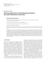
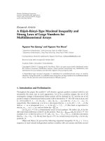
Figure 2: Comparison of analytical and simulated PDFs of SLR
(w
i
is obtained from (32), and the exponential correlation model
is used).
10
−3
10
−2
10
−1
10
0
Outage probability of SLR
−50510
γ
0
(dB)
Theoretical, w
i
from (32)
Simulation, w
i
from (32)

Theoretical, w
i
= (M)
−0.5
ones (M,1)
Theoretical, w
i
= e
λ
m
(G
i
Σ
i
)
Simulation, w
i
= e
λ
m
(G
i
Σ
i
)
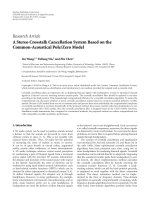
Figure 3: Comparison of outage probablity with different weight
vectors as a function of γ
0
for user i = 1 (exponential correlation
model).

N
i
= N for all i. Note that this is purely by way of example,
and other values could just have easily been considered. The
outage probability of SLR is presented using Monte-Carlo
simulation runs during which the channels (H
i
, i = 1, , K)
change independently and randomly. For each channel
realization, the SLR for ith user is computed and compared
with the threshold value γ
0
for determining the outage
probability.
10
−4
10
−3
10
−2
10
−1
10
0
Outage probability of SLR
−50510
γ
0
(dB)
ρ

1
= 0.4, N = 2theoretical
ρ
1
= 0.4, N = 2 simulation
ρ
1
= 0.98, N = 2theoretical
ρ
1
= 0.98, N = 2 simulation
ρ
1
= 0.4, N = 4theoretical
ρ
1
= 0.4, N = 4 simulation
ρ
1
= 0.98, N = 4theoretical
ρ
1
= 0.98, N = 4 simulation
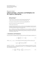
Figure 4: Comparison of theoretical and simulated outage proba-
bility as a function of γ
0
for the user i = 1 (exponential correlation
model).
5.1. Exponential Correlation Model. In this example, the
amplitudes of the spatial correlations among the elements

of the BS antenna array are considered to be exponentially
related. With this assumption, the correlation matrices are
defined as
[
Σ
i
]
mn
= ρ
|m−n|
i
e
−j
(
m−n
)
sin θ
i
, i = 1, ,K, (38)
where m, n
= 1, ,M represent the mth row and nth
column of Σ
i
, ρ
i
are the amplitudes of correlation coefficients
and θ
i
is the AoA of the plane wave from the ith point source.
The analytically obtained PDF (17)ofSLRiscompared

with the simulation results as shown in Figure 2. In this
figure, the beamformer weights are optimized according to
(32) for the exponential correlation model (38). It can be
observed from Figure 2 that the analytical and simulation
results are in fine agreement, and hence the accuracy of
the derived PDF of SLR is validated. Figure 3 displays
the analytical and simulated outage probabilities of SLR
versus γ
0
for (a) the optimized w
i
from (32), (b) the
non-optimized w
i
(w
i
= (1/
√
M)ones(M, 1)), and (c) w
i
which is the eigenvector corresponding to the maximum
eigenvalue of G
i
Σ
i
. Note that the last method simply tries
to maximize the signal power toward the user of interest
without even trying to suppress the leakage power toward
the other users. Although this approach is highly suboptimal,
it is very simple to implement, and its performance can

be encouraging especially in UMTS cellular networks [28]
where, due to downlink omnidirectional strong common
pilot channels, the overall leakage power appears to be almost
8 EURASIP Journal on Wireless Communications and Networking
7.2
7.4
7.6
7.8
8
8.2
8.4
8.6
Average SLR (dB)
0 5 10 15 20 25
N
Exact value
Lower bound
Figure 5: Exact average SLR and its lower bound in (31)asa
function of N for the user i
= 1(w
i
is obtained from (32), and
Gaussian AoA model is used).
0
0.5
1
1.5
2
2.5
3

Cost function
0 5 10 15 20
Angular separation (δ)indegrees
Upper bound, part 1
−r
3
Exact, part 1 −r
1
Upper bound, part 2 −r
4
Exact, part 2 −r
2
Upper bound, total −r
3
+ r
4
Exact total −r
1
+ r
2
Figure 6: Exact cost function and its upper bound in (36)versus
δ for the user i
= 1(w
i
is obtained from (32), and Gaussian AoA
model is used, r
1
= (1/γ
0
) s

con
, r
2
= (1/N)tβ, r
3
= (

K
k
=1,k
/
=i
y
k
/x
i
),
and r
4
= t(K −1)).
white noise. As expected, it can be observed from Figure 3
that the method (32) outperforms the other two cases. The
theoretical and numerical results for different values of ρ
1
and N are compared in Figure 4. In Figures 2 and 3,wetake
ρ
1
= 0.8, and in Figures 2, 3,and4 we take ρ
2
= 0.1, ρ

3
= 0.2,
θ
1
= 45
◦
, θ
2
= 30
◦
,andθ
3
= 60
◦
.
10
−3
10
−2
10
−1
10
0
Outage probability of SLR
−50510
γ
0
(dB)
σ
θ

= 5
◦
,N= 2theoretical
σ
θ
= 5
◦
,N= 2 simulation
σ
θ
= 10
◦
,N= 2theoretical
σ
θ
= 10
◦
,N= 2 simulation
σ
θ
= 5
◦
,N= 4theoretical
σ
θ
= 5
◦
,N= 4 simulation
σ
θ

= 10
◦
,N= 4theoretical
σ
θ
= 10
◦
,N= 4 simulation
Figure 7: Comparison of theoretical and simulated outage proba-
bility as a function of γ
0
for user i = 1(w
i
is obtained from (32)and
Gaussian AoA model is used).
5.2. Spatial Correlation Model-Gaussian Angle of Arrival
(AoA). In this example, the spatial correlation among ele-
ments of the BS antenna array is modeled according to
the distribution of the AoA of the incoming plane waves
at the BS from the ith user. The AoA is assumed to be
Gaussian distributed with a standard deviation σ
i
θ
of angular
spreading. For this case, we consider a uniform linear array
with the half-wavelength spacing. The correlation is thus
given by [3]
[
Σ
i

]
mn
= e
jπ
(
m−n
)
sin θ
i
e
−
(
π
(
m−n
)
σ
i
θ
cos θ
i
)
2
/2
, i = 1, ,K,
(39)
where θ
i
is the central angle of the incoming rays to the BS
from the ith user. We assume that the first user is located at

θ
1
= 10
◦
relative to the BS array broadside, and the other
two users are located at θ
2,3
= 10
◦
± δ where we take δ = 8
◦
(except in Figure 6 where δ is varied) and σ
i
θ
= σ
θ
for all i.
The exact average SLR (27) and its lower bound (31)
both versus N are compared in Figure 5 where the optimum
weight vector is chosen according to (32). We take σ
θ
=
3
◦
for this figure. It can be seen from Figure 5, that the
difference between the exact values of the average SLR and
its lower bound is almost negligible for all N which in fact
confirms that the beamformer (32) maximizes the average
SLRwithaveryfineaccuracy.Theexactfunctionsin(28)and
(35), their corresponding upper bounds, the sum function

(36)(witht
= 1), and its upper bound are displayed in
Figure 6 for different values of δ where the beamformer is
derived from (32). It can be observed from this figure that
EURASIP Journal on Wireless Communications and Networking 9
−10
−5
0
5
10
15
Average SINR (dB)
−505101520
−10
∗
log 10(σ
2
i
)(dB)
(a)
−15
−10
−5
0
5
10
Average SLNR (dB)
−505101520
−10
∗

log 10(σ
2
i
)(dB)
w
i
from (32)
w
i
= e
λ
m
(G
i
Σ
i
)
w
i
= (M)
−0.5
ones (M,1)
(b)
Figure 8:AverageSINRandaverageSLNRversusnoisepowerfor
the user i
= 1 (Gaussian AoA model with σ
θ
= 3
◦
).

the bound in (28)isverytightforallvaluesofδ whereas
that in (35) is tight for the medium and larger values of
δ. In fact, the gap between the overall exact function (36)
and its upper bound is sufficiently small for all values of
δ. Figure 7 shows the outage probability of SLR versus γ
0
obtained via theory and simulations for different values of
σ
θ
and N. The average SINR (5) and the average SLNR (3)
of ith user versus the receiver noise power σ
2
i
are displayed
in Figure 8 again for (a) the optimized w
i
of (32), (b) the
non-optimized w
i
(w
i
= (1/
√
M)ones(M, 1)), and (c) w
i
which is the eigenvector corresponding to the maximum
eigenvalue of G
i
Σ
i

. In this figure, the SINR and SLNR are
averaged over 10
4
independent channel realizations, and
it is considered that the receiver has perfect knowledge
of instantaneous channels. It can be seen from Figure 8
that the transmit beamformer (32) based on maximiza-
tion of SLR significantly helps to improve the receiver’s
SINR. Figures 3, 4,and7 display that the matching between
the theoretical and simulation results is very fine. This
confirms the validity of the proposed theoretical expression
for outage probability. It can be noticed (see Figures 3
and 8) that the beamformer, which tries to suppress the
leakage power while maximizing the signal power (32),
is better than the one which only maximizes the signal
power of the user of interest by neglecting the leakage
power (method (c)). The results (Figures 4 and 7) also
show that as the spatial correlation between the antenna
elements increases (correlation coefficient increases or angu-
lar spreading decreases), the outage probability decreases.
The latter observation can be explained from the fact that
when the spatial correlation increases, the ranks of MIMO
channels decrease, thereby allowing the beamformer to
performbetter.Thebestperformancecanevenbeobtained
when the MIMO channels are fully correlated ( i.e., channels
become rank one). It can be also observed (see Figures 4
and 7) that by increasing the BS antenna correlation, the
performance can be improved more effectively than just
by increasing the number of user antennas while keeping
the BS antenna correlation sufficiently low. Furthermore,

as expected in Figures 3, 4,and7, the outage probability
increases with increasing γ
0
.
6. Conclusions
A fine agreement between the theoretical and simulation
results for the PDF of SLR and its outage probability confirms
the correctness of the proposed analysis for a multiuser
MIMO downlink beamforming in a Rayleigh fading envi-
ronment. The results also show that the spatial correlation
between the antenna elements significantly helps to increase
the performance of the SLR-based transmit beamformer
in terms of the SLR outage probability. It has been found
via some approximations that the transmit beamformer
which maximizes the average SLR also minimizes the outage
probability of the SLR.
References
[1] F. Rashid-Farrokhi, K. J. R. Liu, and L. Tassiulas, “Joint optimal
power control and beamforming in wireless networks using
antenna arrays,” IEEE Transactions on Communications, vol.
46, no. 10, pp. 1313–1324, 1998.
[2] M. Schubert and H. Boche, “Solution of the multiuser down-
link beamforming problem with individual SINR constraints,”
IEEE Transactions on Vehicular Technology,vol.53,no.1,pp.
18–28, 2004.
[3] M. Bengtsson and B. Ottersten, “Optimal downlink beam-
forming using semidefinite optimization,” in Proceedings of the
37th Annual Allerton Conference on Communication, Control,
and Computing, pp. 987–996, Monticello, Ill, USA, September
1999.

[4] G. J. Foschini, “Layered space-time architecture for wireless
communication in a fading environment when using multi-
element antennas,” Bell Labs Technical Journal, vol. 1, no. 2,
pp. 41–59, 1996.
[5] E. Telatar, “Capacity of multi-antenna Gaussian channels,”
European Transactions on Telecommunications, vol. 10, no. 6,
pp. 585–595, 1999.
[6] J H. Chang, L. Tassiulas, and F. Rashid-Farrokhi, “Joint
transmitter receiver diversity for efficient space division
multiaccess,” IEEE Transactions on Wireless Communications,
vol. 1, no. 1, pp. 16–27, 2002.
[7] M. Sadek, A. Tarighat, and A. H. Sayed, “A leakage-based
precoding scheme for downlink multi-user MIMO channels,”
IEEE Transactions on Wireless Communications, vol. 6, no. 5,
pp. 1711–1721, 2007.
[8] M.Sadek,A.Tarighat,andA.H.Sayed,“Activeantennaselec-
tion in multiuser MIMO communications,” IEEE Transactions
on Signal Processing, vol. 55, no. 4, pp. 1498–1510, 2007.
[9] D. Gerlach and A. Paulraj, “Base station transmitting antenna
arrays for multipath environments,” Signal Processing, vol. 54,
no. 1, pp. 59–73, 1996.
10 EURASIP Journal on Wireless Communications and Networking
[10] P. Zetterberg and B. Ottersten, “The Spectrum efficiency of
a base station antenna array system for spatially selective
transmission,” IEEE Transactions on Vehicular Technology, vol.
44, no. 3, pp. 651–660, 1995.
[11] M. Bengtsson and B. Ottersten, “Optimal and suboptimal
beamforming,” in Handbook of Antennas in Wireless Commu-
nications, CRC Press, Boca Raton, Fla, USA, August 2001.
[12] Y. Song, S. D. Blostein, and J. Cheng, “Exact outage probability

for equal gain combining with cochannel interference in
Rayleigh fading,” IEEE Transactions on Wireless Communica-
tions, vol. 2, no. 5, pp. 865–870, 2003.
[13] A. Shah and A. M. Haimovich, “Performance analysis of opti-
mum combining in wireless communications with rayleigh
fading and cochannel interference,” IEEE Transactions on
Communications, vol. 46, no. 4, pp. 473–479, 1998.
[14] A. Shah and A. M. Haimovich, “Performance analysis of
maximal ratio combining and comparison with optimum
combining for mobile radio communications with cochannel
interference,” IEEE Transactions on Vehicular Technology, vol.
49, no. 4, pp. 1454–1463, 2000.
[15] S. Kandukuri and S. Boyd, “Optimal power control in
interference-limited fading wireless channels with outage-
probability specifications,” IEEE Transactions on Wireless Com-
munications, vol. 1, no. 1, pp. 46–55, 2002.
[16] J. Papandriopoulos, J. Evans, and S. Dey, “Outage-based opti-
mal power control for generalized multiuser fading channels,”
IEEE Transactions on Communications, vol. 54, no. 4, pp. 693–
703, 2006.
[17] M. Bengtsson and B. Ottersten, “Signal waveform estimation
from array data in angular spread environment,” in Proceed-
ings of the 13th Asilomar Conference on Signals, Systems and
Computers, vol. 1, pp. 355–359, November 1997.
[18] S. Zhou and G. B. Giannakis, “Optimal transmitter eigen-
beamforming and space-time block coding based on channel
correlations,” IEEE Transactions on Information Theory, vol.
49, no. 7, pp. 1673–1690, 2003.
[19] M. Chiani, M. Z. Win, and A. Zanella, “On the capacity of
spatially correlated MIMO Rayleigh-fading channels,” IEEE

Transactions on Information Theory, vol. 49, no. 10, pp. 2363–
2371, 2003.
[20] J. Luo, J. R. Zeidler, and S. McLaughlin, “Performance analysis
of compact antenna arrays with MRC in correlated Nakagami
fading channels,” IEEE Transactions on Vehicular Technology,
vol. 50, no. 1, pp. 267–277, 2001.
[21] L. H
¨
aring, B. K. Chalise, and A. Czylwik, “Dynamic system
level simulations of downlink beamforming for UMTS FDD,”
in Proceedings of IEEE Global Telecommunications Conference
(GLOBECOM ’03), vol. 1, pp. 492–496, San Francisco, Calif,
USA, December 2003.
[22] H. Rong and K. Hiltunen, “Performance investigation of sec-
ondary scrambling codes in WCDMA systems,” in Proceedings
of the 63rd IEEE Vehicular Technology Conference (VTC ’06),
vol. 2, pp. 698–702, Melbourne, Australia, May 2006.
[23] R. J. Muirhead, Aspects of Multivariate Statistical Theory,Wiley
Series in Probability and Mathematical Statistics, Wiley, New
York, NY, USA, 1982.
[24] Q. T. Zhang and D. P. Liu, “A simple capacity formula for
correlated diversity Rician fading channels,” IEEE Communi-
cations Letters, vol. 6, no. 11, pp. 481–483, 2002.
[25] I. S. Gradshteyn and I. M. Ryzhik, Table of Integrals, Ser ies, and
Products, Academic Press, New York, NY, USA, 6th edition,
2000, A. Jeffrey Ed.
[26] A. P. Iserte, A. I. Perez-Neira, and M. A. L. Hernandez,
“Joint beamforming strategies in OFDM-MIMO systems,”
in Proceedings of IEEE International Conference on Acoustics,
Speech, and Signal Processing (ICASSP ’02), vol. 3, pp. 2845–

2848, Orlando, Fla, USA, May 2002.
[27] S. Boyd and L. Vandenbergh, Convex Optimization,Cam-
bridge University Press, Cambridge, UK, 2004.
[28] A. Czylwik, A. Dekorsy, and B. K. Chalise, “Smart antenna
solutions for UMTS,” in Smart Antennas—State of the Art,
T. Kaiser, A. Boudroux, et al., Eds., EURASIP Hindawi Book
Series, pp. 729–758, 2005.