Báo cáo hóa học: "Research Article Practical Gammatone-Like Filters for Auditory Processing" docx

Hindawi Publishing Corporation
EURASIP Journal on Audio, Speech, and Music Processing
Volume 2007, Article ID 63685, 15 pages
doi:10.1155/2007/63685
Research Article
Practical Gammatone-Like Filters for Auditory Processing
A. G. Katsiamis,
1
E. M. Drakakis,
1
andR.F.Lyon
2
1
Department of Bioengineering, The Sir Leon Bagrit Centre, Imperial College London, South Kensington Campus,
London SW7 2AZ, UK
2
Google Inc., 1600 Amphitheatre Parkway Mountain View, CA 94043, USA
Received 10 October 2006; Accepted 27 August 2007
Recommended by Jont B. Allen
This paper deals with continuous-time filter transfer functions that resemble tuning curves at particular set of places on the basilar
membrane of the biological cochlea and that are suitable for practical VLSI implementations. The resulting filters can be used in
a filterbank architecture to realize cochlea implants or auditory processors of increased biorealism. To put the reader into context,
the paper starts with a short review on the gammatone filter and then exposes two of its variants, namely, the differentiated all-pole
gammatone filter (DAPGF) and one-zero gammatone filter (OZGF), filter responses that provide a robust foundation for modeling
cochlea transfer functions. The DAPGF and OZGF responses are attractive because they exhibit certain characteristics suitable for
modeling a variety of auditory data: level-dependent gain, linear tail for frequencies well below the center frequency, asymmetry,
and so forth. In addition, their form suggests their implementation by means of cascades of N identical two-pole systems which
render them as excellent candidates for efficient analog or digital VLSI realizations. We provide results that shed light on their char-
acteristics and attributes and which can also serve as “design curves” for fitting these responses to frequency-domain physiological
data. The DAPGF and OZGF responses are essentially a “missing link” between physiological, electrical, and mechanical models
for auditory filtering.

Copyright © 2007 A. G. Katsiamis et al. This is an open access article distributed under the Creative Commons Attribution
License, which permits unrestricted use, distribution, and reproduction in any medium, provided the original work is properly
cited.
1. INTRODUCTION
For more than twenty years, the VLSI community has been
performing extensive research to comprehend, model, and
design in silicon naturally encountered biological auditory
systems and more specifically the inner ear or cochlea. This
ongoing effort aims not only at the implementation of the ul-
timate artificial auditory processor (or implant), but also to
aid our understanding of the underlying engineering princi-
ples that nature has applied through years of evolution. Fur-
thermore, parts of the engineering community believe that
mimicking certain biological systems at architectural and/or
operational level should in principle yield systems that share
nature’s power-efficient computational ability [1]. Of course,
engineers bearing in mind what can be practically realized
must identify what should and what should not be blindly
replicated in such a “bioinspired” artificial system. Just as it
does not make sense to create flapping airplane wings only to
mimic birds’ flying, it seems equally meaningful to argue that
not all operations of a cochlea can or should be replicated
in silicon in an exact manner. Abstractive operational or ar-
chitectural simplifications dictated by logic and the available
technology have been crucial for the successful implementa-
tion of useful hearing-type machines.
A cochlea processor can be designed in accordance with
two well-understood and extensively analyzed architectures:
the parallel filterbank and the traveling-wave filter cascade. A
multitude of characteristic examples representative of both

architectures have been reported [2–6]. Both architectures
essentially perform the same task; they analyze the incom-
ing spectrum by splitting the input (audio) signal into sub-
sequent frequency bands exactly as done by the biologi-
cal cochlea. Moreover, transduction, nonlinear compression,
and amplification can be incorporated in both to model ef-
fectively inner- and outer-hair-cells (IHC and OHC, resp.)
operation yielding responses similar to the ones observed
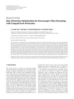
from the biological cochleae. Figure 1 illustrates how basilar
membrane (BM) filtering is modeled in both architectures.
2. MOTIVATION: ANALOG VERSUS DIGITAL
Hearing is a perceptive task and nature has developed an effi-
cient strategy in accomplishing it: theadaptivetraveling-wave
2 EURASIP Journal on Audio, Speech, and Music Processing
amplifier structure. Bioinspired analog circuitry is capable of
mimicking the dynamics of the biological prototype with
ultra-low power consumption in the order of tens of μWs
(comparable to the consumption of the biological cochlea).
Comparative calculations would show that opting for a cus-
tom digital implementation of the same dynamics would still
cost us considerably more in terms of both silicon area and
power consumption [7]; power consumption savings of at
least two orders of magnitude and silicon area savings of at
least three can be expected should ultra-low power analog
circuitry be used effectively. This is due to the fact that in
contrast to the power hungry digital approaches, where a sin-
gle operation is performed out of a series of switched-on or
-off transistors, the individual devices are treated as analog
computational primitives; operational tasks are performed in
a continuous-time analog way by direct exploitation of the

physics of the elementary device. Hence, the energy per unit
computation is lower and power efficiency is increased. How-
ever, for high-precision simulation, digital is certainly more
energy-efficient [8].
Apart from that, realizing filter transfer functions in the
digital domain does not impose severe constraints and trade-
offs to the designer apart from stability issues. For exam-
ple, in [9], a novel application of a filtering design technique
that can be used to fit measured auditory tuning curves was
proposed. Auditory filters were obtained by minimizing the
squared difference, on a logarithmic scale, between the mea-
sured amplitude of the nerve tuning curve and the magni-
tude response of the digital IIR filter. Even though this ap-
proach will shed some light on the kind of filtering the real
cochlea is performing, such computational techniques are
not suited for analog realizations.
Moreover, different analog design synthesis techniques
(switched-capacitor, Gm-C, log-domain, etc.) yield different
practical implementations and impose different constraints
on the designer. For example, it is well known that realizing
finite transmission zeros in a filter’s transfer function using
the log-domain circuit technique is a challenging task [10].
As such, and with the filterbank architecture in mind,
finding filter transfer functions that have the potential for an
efficient analog implementation while grasping most of the
biological cochlea’s operational attributes is the focus of this
and our ongoing work. It goes without saying that the design
of these filters in digital hardware (or even software) will be
a much simpler task than in analog.
3. COCHLEA NONLINEARITY: BM RESPONSES

The cochlea is known to be a nonlinear, causal, active system.
It is active since it contains a battery (the difference in ionic
concentration between scala vestibuli, tympani, and media,
called the endocochlear potential, acts as a silent power sup-
ply for the hair cells in the organ of Corti) and nonlinear
as evidenced by a multitude of physiological characteristics
such as generating otoacoustic emissions.
In 1948, Thomas Gold (22 May 1920–1922 June 2004), a
distinguished cosmologist, geophysicist, and original thinker
with major contributions to theories of biophysics, the origin
of the universe, the nature of pulsars, the physics of the mag-
netosphere, the extra terrestrial origins of life on earth, and
much more, argued that there must be an active, undamping
mechanism in the cochlea, and he proposed that the cochlea
had the same positive feedback mechanism that radio engi-
neers applied in the 1920s and 1930s to enhance the selectiv-
ity of radio receivers [11, 12]. Gold had done army-time work
on radars and as such he applied his signal-processing knowl-
edge to explain how the ear works. He knew that to preserve
signal-to-noise ratio, a signal had to be amplified before the
detector. “Surely nature cannot be as stupid as to go and put
a nerve fiber—the detector—right at the front end of the sen-
sitivity of the system,” Gold said. Gold had his idea back in
1946, while being a graduate astrophysicist student at Cam-
bridge University, England. He spotted a flaw in the classical
theory of hearing (the sympathetic resonance model) devel-
oped by Hermann von Helmholtz [13]almostacenturybe-
fore. Helmholtz’s theory assumed that the inner ear consists
of a set of “strings,” each of which vibrates at a different fre-
quency. Gold, however, realized that friction would prevent

resonance from building up and that some active process is
needed to counteract the friction. He argued that the cochlea
is “regenerative” adding energy to the very signal that it is
trying to detect. Gold’s theories also daringly challenged von
B
´
ek
´
esy’s large-scale traveling-wave cochlea models [14]and
he was also the first to predict and study otoacoustic emis-
sions. Ignored for over 30 years, his research was rediscov-
ered by a British engineer by the name of David Kemp, who
in 1979 proposed the “active” cochlea model [15]. Kemp sug-
gested that the cochlea’s gain adaptation and sharp tuning
were due to the OHC operation in the organ of Corti.
Early physiological experiments (Steinberg and Gardner
1937 [16]) showed that the loss of nonlinear compression in
the cochlea leads to loudness recruitment.
1
Moreover, it can
be shown that the dynamic range of IHC (the cochlea’s trans-
ducers) is about 60 dB rendering them inadequate to process
the achieved 120 dB of input dynamic range without signal
compression. It is by now widely accepted that the 6 orders
of magnitude of input acoustic dynamic range supported by
the human ear are due to OHC-mediated compression.
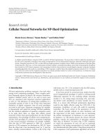
Evidence for the cochlea nonlinearity was first given by
Rhode.Inhispapers[17, 18], he demonstrated BM mea-
surements yielding cochlea transfer functions for different
input sound intensities. He observed that the BM displace-

ment (or velocity) varied highly nonlinearly with input level.
More specifically, for every four dBs of input sound pres-
sure level (SPL) increase, the BM displacement (or veloc-
ity) as measured at a specific BM place changed only by one
dB. This compressive nonlinearity was frequency-dependent
and took place only near the most sensitive frequency region,
the peak of the tuning curve. For other frequencies, the sys-
tem behaved linearly; that is, one dB change in input SPL
yielded one dB of output change for frequencies away from
the center frequency. In addition, for high input SPL, the
1
Loudness recruitment occurs in some ears that have high-frequency hear-
ing loss due to a diseased or damaged cochlea. Recruitment is the rapid
growth of loudness of certain sounds that are near the same frequency of
a person’s hearing loss.
A. G. Katsiamis et al. 3
Channel 1
Channel 2
Channel 3
Channel m
APEX
Basilar
membrane
f
m
f
3
f
2
f

1
BASE
f
f
f
Filterbank
architecture
Exponential decrease of centre frequencies
Ta p m Ta p 3 Ta p 2 Ta p 1 f
Input
Input
Filter-cascade architecture
Figure 1: Graphical representation of the filterbank and filter-cascade architectures. The filters in the filter-cascade architecture have non-
coincident poles; their cut-off frequencies are spaced-out in an exponentially decreasing fashion from high to low. On the other hand, the
filter cascades per channel of the filterbank architecture have identical poles. However, each channel follows the same frequency distribution
as in the filter-cascade case.
high-frequency roll-off slope broadened (the selectivity de-
creased) with a shift of the peak towards lower frequencies,
in contrast to low input intensities where it became steeper
(the selectivity increased) with a shift of the peak towards
higher frequencies. Figure 2 illustrates these results.
From the engineering point of view, we seek filters whose
transfer functions can be controlled in a similar manner, that
is,
(i) low input intensity
→ high gain and selectivity and
shift of the peak to the “right” in the frequency do-
main;
(ii) high input intensity
→ low gain and selectivity and

shift of the peak to the “left” in the frequency domain.
As a first rough approximation of the above behavior,
it is worth noting that the simplest VLSI-compatible reso-
nant structure, the lowpass biquadratic filter (LP biquad),
gives a frequency response that exhibits this kind of level-
dependent compressive behavior by varying only one param-
eter, its quality factor. The standard LP biquad transfer func-
tion is
H
LP
(s) =
ω
2
o
s
2
+

ω
o
/Q

s + ω
2
o
,(1)
where ω
o
is the natural (or pole) frequency and Q is the qual-
ity factor. The frequency, where the peak gain occurs or cen-

ter frequency (CF) is related to the natural frequency and Q,
is as follows:
ω
LP
CF
= ω
o

1 −
1
2Q
2
,(2)
024681012141618
×10
3
Frequency (Hz)
10
−1
10
0
10
1
10
2
10
3
Gain (mm/s/Pa)
0dBSPL
10 dB SPL

20 dB SPL
30 dB SPL
40 dB SPL
50 dB SPL
60 dB SPL
70 dB SPL
80 dB SPL
90 dB SPL
100 dB SPL
Figure 2: Frequency-dependent nonlinearity in BM tuning curves,
adapted from Ruggero et al. [19].
suggesting the lowest Q value of 1/
√
2 for zero CF. The LP bi-
quad peak gain can be parameterized in terms of Q according
to
H
LP
max
=
Q

1 −1/4Q
2
. (3)
4 EURASIP Journal on Audio, Speech, and Music Processing
10
−1
10
0

Normalized frequency
−5
0
5
10
15
20
Lowpass biquad filter gain (dB)
Lowpass biquad filter frequency response
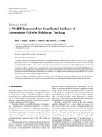
Figure 3: The LP biquad transfer function illustrating level-
dependent gain with single parameter variation. The dotted line
shows roughly how the peak shifts to the right as gain increases.
The frequency axis is normalized to the natural frequency.
Figure 3 shows a plot of the LP biquad transfer function with
Q varying from 1/
√
2 to 10. Observe that as Q increases, ω
LP
CF
tends to be closer to ω
o
modeling the shift of the peak to-
wards high frequencies as intensity decreases.
4. REFERENCE MEASURES OF BM RESPONSES
With such a plethora of physiological measurements (not
only from various animals but also from several experimen-
tal methods), it is practically impossible to have universal
and exquisitely insensitive measures which define cochlea
biomimicry and act as “reference points.” In other words,
it seems that we do not have an absolute BM measurement

against which all the responses from our artificial systems
could be compared. Eventually, a biomimetic design will
be the one which will have the potential to achieve perfor-
mances of the same order of magnitude to those obtained
from the biological counterparts. The goal is not necessarily
the faithful reproduction of every feature of the physiological
measurement, but just of the right ones. Of course, the right
features are not known in advance; so there must be an ac-
tive collaboration between the design engineers, the cochlea
biophysicists, and those who treat and test the beneficiaries
of the engineering efforts. To aid our discussion, we resort to
Rhode’sBMresponsemeasuredefinedin[20].
Rhode observed that the cochlea transfer function at a
particular place in the BM is neither purely lowpass nor
purely bandpass. It is rather an asymmetric bandpass func-
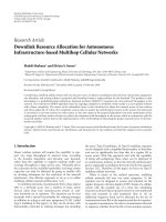
tion of frequency. He thus defined a graph, such as the one
shown in Figure 4, where all tuning curves can be fitted by
straight lines on log-log coordinates. The slopes (S1, S2, and
S3), as well as the break points (ω
Z
and ω
CF
) defined as the
locations where the straight lines cross, characterize a given
response. Ta b le 1 ,adaptedfromAllen[21] and extended
ω
z
ω
CF
S3

S2
S1
Frequency
Excess gain
Gain (dB)
Figure 4: Rhode’s BM frequency response measure, a piecewise ap-
proximation of the BM frequency response.
here, gives a summary of this parametric representation of
BM responses from various sources.
Observe that ω
Z
usually ranges between 0.5 and 1 oc-
tave below ω
CF
, the slopes S1 and S2 range between 6 and
12 dB/oct and 20 and 60 dB/oct, respectively, and S3 is lower
than at least
−100 dB/oct. In other words, it seems that S1
corresponds to a first- or second-order highpass frequency
shaping LTI network, S2 to at least a fourth- (up to tenth-
)orderone,andS3 to at least a seventeenth-order lowpass
response. The minimum excess gain of
∼18 dB corresponds
approximately to the peak gain of an LP biquad response
with a Q value of 10.
Other BM measures, more insensitive to many impor-
tant details and also more prone to experimental errors, are
the Q
10
(or Q

3
) defined as the ratio of CF over the 10 dB or
3 dB bandwidth, respectively, and the “tip-to-tail ratio” rela-
tive to a low-frequency tail taken about an octave below the
CF. Tab le 1 provides a good idea of what should be mimicked
in an artificial/engineered cochlea. Filter transfer functions,
which
(i) can be tuned to have parameter values similar/compa-
rable to the ones presented in Tab le 1,
(ii) are gain-adjustable by varying as few parameters as
possible (ideally one parameter),
(iii) are suited in terms of practical complexity for VLSI
implementation,
are what we ultimately seek to incorporate in an artificial
VLSI cochlea architecture. In the following sections, a gen-
eral class of such transfer functions is introduced and their
properties are studied in detail.
5. THE GAMMATONE AUDITORY FILTERS
The gammatone (or Γ-tone) filter (GTF) was introduced by
Johannesma in 1972 to describe cochlea nucleus response
[25]. A few years later, de Boer and de Jongh developed the
gammatone filter to characterize physiological data gathered
from reverse-correlation (Revcor) techniques from primary
auditory fibers in the cat [26, 27].
A. G. Katsiamis et al. 5
Table 1: Parametric representation of BM responses from various sources.
Data type Reference log
2
( f
z

/f
Cf
)(oct) S1(dB/oct) Max(S2) (dB/oct) Max(S3)(dB/oct) Excessgain(dB)
Conditions
Input SPL (dB) f
CF
(kHz)
BM [17] — 6 20 –100 28 80 7
BM [20] 0.57 9 86 –288 27 50–105 7.4
BM [22] 0.88 10 28 –101 17.4 20–100 15
BM [23] 0.73 12 48.9 –110 32.5 10–90 10
BM [23] 0.44 8 53.9 –286 35.9 0–100 9.5
Neural [24] 0.5–0.8 0–10 50–170 < –300 50–80 — >3
Table 2: Gammatone filter variants’ transfer functions.
Filter type Transfer function
GTF H
GTF
(s) =
e
jϕ

s + ω
o
/2Q + jω
o

1 − 1/4Q
2

N

+ e
−jϕ

s + ω
o
/2Q − jω
o

1 − 1/4Q
2

N

s
2
+

ω
o
/Q

s + ω
2
o

N
(4)
APGF H
APGF
(s) =

K

s
2
+

ω
o
/Q

s + ω
2
o

N
, K = ω
2N
o
for unity gain at DC (5)
DAPGF H
DAPGF
(s) =
Ks

s
2
+

ω
o

/Q

s + ω
2
o

N
, K = ω
2N−1
o
for dimensional consistency (6)
OZGF H
OZGF
(s) =
K

s + ω
z


s
2
+

ω
o
/Q

s + ω
2

o

N
, K = ω
2N−1
o
for dimensional consistency (7)
However, Flanagan was the first to use it as a BM model
in [28], but he neither formulated nor introduced the name
“gammatone” even though it seems he had understood its
key properties. Its name was given by Aertsen and Johan-
nesma in [29] after observing the nature of its impulse re-
sponse. Since then, it has been adopted as the basis of a num-
ber of successful auditory modeling efforts [30–33]. Three
factors account for the success and popularity of the GTF in
the audio engineering/speech-recognition community:
(i) it provides an appropriately shaped “pseudoresonant”
[34] frequency transfer function making it easy to
match reasonably well-measured responses;
(ii) it has a very simple description in terms of its time-
domain impulse response (a gamma-distribution en-
velope times a sinusoidal tone);
(iii) it provides the possibility for an efficient hardware im-
plementation.
The gammatone impulse response with its constituent
components is shown in Figure 5. Note that for the gamma-
distribution factor to be an actual probability distribution
(i.e., to integrate to unity), the factor A needs to be b
N
/Γ(N),

with the gamma function being defined for integers as the
factorial of the next lower integer Γ(N)
= (N −1)!. In prac-
tice, however, A is used as an arbitrary factor in the filter re-
sponse and it is typically chosen to make the peak gain equal
unity.
The gamma-distribution At
N−1
exp (−bt)
The tone cos

ω
r
t + ϕ

The gammatone At
N−1
e
(−bt)
cos

ω
r
t + ϕ

(8)
0246810
Time
0
0.2

0.4
Arbitrary
units
The GTF impulse response and its components
(a)
0246810
Time
−1
0
1
Arbitrary
units
(b)
0246810
Time
−0.5
0
0.5
Arbitrary
units
(c)
Figure 5: The components of a gammatone filter impulse response;
the gamma-distribution envelope (top); the sinusoidal tone (mid-
dle); the gammatone impulse response (bottom).
The parameters’ order N (integer), ringing frequency ω
r
(rad/s), starting phase ϕ (rad), and one-sided pole band-
width b (rad/s), together with (8), complete the description
of the GTF.
6 EURASIP Journal on Audio, Speech, and Music Processing

Three key limitations of the GTF are as follows.
(i) It is inherently nearly symmetric, while physiological
measurements show a significant asymmetry in the au-
ditory filter (see Section 6.5 for a more detailed de-
scription regarding asymmetry).
(ii) It has a very complex frequency-domain description
(see (4)). Therefore, it is not easy to use parameteriza-
tion techniques to realistically model level-dependent
changes (gain control) in the auditory filter.
(iii) Due to its frequency-domain complexity, it is not easy
to implement the GFT in the analog domain.
Lyon presented in [35] a close relative to the GTF, which
he termed as all-pole gammatone filter (APGF) to highlight
its similarity to and distinction from the GTF.
The APGF can be defined by discarding the zeros from
a pole-zero decomposition of the GTF—all that remains is
a complex conjugate pair of Nth-order poles (see (5)). The
APGF was originally introduced by Slaney [36]asan“all-
pole gammatone approximation,” an efficient approximate
implementation of the GTF, rather than as an important fil-
ter in its own right.
In this paper, we will expose the differentiated all-pole
gammatone filter (DAPGF) and the one-zero gammatone fil-
ter (OZGF) as better approximations to the GTF, which in-
herits all the advantages of the APGF. It is worth noting that
a third-order DAPGF was first used to model BM motion
by Flanagan [28], as an alternative to the third-order GTF.
The DAPGF is defined by multiplying the APGF with a dif-
ferentiator transfer function to introduce a zero at DC (i.e.,
at s

= 0 in the Laplace domain) (see (6)), whereas the OZGF
has a zero anywhere on the real axis (i.e., s
= α for any real
value α) (see (7)).
The APGF, DAPGF, and OZGF have several properties
that make them particularly attractive for applications in au-
ditory modeling:
(i) they exhibit a realistic asymmetry in the frequency do-
main, providing a potentially better match to psychoa-
coustic data;
(ii) they have a simple parameterization;
(iii) with a single level-dependent parameter (their Q), they
exhibit reasonable bandwidth and center frequency
variation, while maintaining a linear low-frequency
tail;
(iv) they are very efficiently implemented in hardware and
particularly in analog VLSI;
(v) they provide a logical link to Lyon’s neuromorphic and
biomimetic traveling-wave filter-cascade architectures.
Ta bl e 2 summarizes GTF, APGF, DAPGF, and OZGF with
their corresponding transfer functions.
6. OBSERVATIONS ON THE DAPGF RESPONSE
The DAPGF can be considered as a cascade of (N
− 1) iden-
tical LP biquads (i.e., an (N
− 1)th-order APGF) and an ap-
propriately scaled BP biquad. Therefore, the DAPGF is char-
acterized as a complex conjugate pair of Nth-order pole loca-
tions with an additional zero location at DC. Unfortunately,
10

−1
10
0
Normalized frequency
−30
−20
−10
0
10
20
30
40
50
60
70
Gain (dB)
4th-order DAPGF
3rd-order APGF
BP biquad
Figure 6: Transfer function of the DAPGF of N = 4andQ = 10,
its decomposition to a third-order APGF, and a scaled BP biquad
with a gain of 20 dB. The frequency axis is normalized to the natural
frequency.
this zero does not make the analytical description of the
DAPGF as straightforward as in the case of the APGF (which
is just an LP biquad raised to the Nth power). The DAPGF
transfer function is
H
DAPGF
(s) =

K
1

s
2
+

ω
o
/Q

s + ω
2
o

N−1
×
K
2
s
s
2
+

ω
o
/Q

s + ω
2

o
=
Ks

s
2
+

ω
o
/Q

s + ω
2
o

N
=
ω
2N−1
o
s

s
2
+

ω
o
/Q


s + ω
2
o

N
.
(9)
Note that the constant gain term K
= K
1
K
2
was chosen to be
ω
2N−1
o
in order to preserve dimensional consistency and aid
implementation. Specifically, K
1
= ω
2(N−1)
o
and K
2
= ω
o
.
Figure 6 illustrates that an Nth-order DAPGF, as defined
previously, has both its peak gain and CF larger than its con-

stituent (N
− 1)th-order APGF. Its larger peak is due to the
fact that the BP biquad is appropriately scaled (for 0 dB BP
biquad gain; K
2
should be ω
o
/Q, whereas here we set it to
be ω
o
) in order to maintain a constant gain across levels for
the low-frequency tail as observed physiologically [17, 37]. In
addition, since an Nth-order DAPGF consists of (N
−1) cas-
caded LP biquads, it is reasonable to expect that the DAPGF
will have a behavior closely related to the LP biquad’s in
terms of how its gain and selectivity change with varying Q
values. Figure 7 illustrates this behavior.
Since the DAPGF can be characterized by two parame-
ters only (N and Q), it would be very convenient to codify
graphically how these parameters depend on each other and
how their variation can achieve a given response that best fits
A. G. Katsiamis et al. 7
10
−2
10
−1
10
0
Normalized frequency

−40
−20
0
20
40
60
80
DAPGF gain (dB)
The DAPGF frequency response
Figure 7: The DAPGF frequency response of N = 4 with Q ranging
from 0.75 to 10. The frequency axis is normalized to the natural
frequency.
physiological data. In the following sections, we derive ex-
pressions for the peak gain, CF, bandwidth, and low-side dis-
persioninanattempttocharacterizetheDAPGFresponse
and create graphs which show how Q can be traded off with
N (and vice versa) to achieve a given specification.
6.1. Magnitude response: peak gain iso-N responses
The DAPGF can be characterized by its magnitude transfer
function


H
DAPGF
(jω)


=

H

DAPGF
(jω) ×H
∗
DAPGF
(jω)
=
ω
2N−1
o
ω

ω
4
−2

1 −1/2Q
2

ω
2
o
ω
2
+ ω
4
o

N/2
.
(10)

Differentiating (10)withrespecttoω and setting it to zero
will give the DAPGF CF ω
DAPGF
CF
. Fortunately, the above dif-
ferentiation results in a quadratic polynomial which can be
solved analytically:
d


H
DAPGF
(jω)


ω
= 0
=⇒ ω
4
−2

N −1
2N −1

1 −
1
2Q
2

ω

2
o
ω
2
−
ω
4
o
2N −1
= 0
=⇒ ω
DAPGF
CF
= ω
o


N −1
2N −1

1 −
1
2Q
2

×







1+




1+
1

(N −1)
2
/(2N − 1)

1 −1/2Q
2

2

.
(11)
11.522.533.5
DAPGF stage Q
0.5
0.6
0.7
0.8
0.9
1
CF normalized to natural frequency

CF normalized to natural frequency iso-N responses
2
4
8
16
N
= 32
Figure 8: DAPGF CF normalized to natural frequency iso-N re-
sponses for varying Q values. For high Q values, the behavior be-
comes asymptotic.
From (11), it is not exactly clear if the DAPGF has a similar
behavior to the LP biquad in terms of how its CF approaches
ω
o
in the frequency domain as Q increases. Figure 8 shows
ω
DAPGF
CF
/ω
o
iso-N responses for varying Q values. Observe
that as N tends to large values and (11) tends to (2), that
is, for large N, the behavior is exactly that of the LP biquad
(or APGF). Note that for N
= 32 and for Q<1, ω
DAPGF
CF
/ω
o
is close to 0.5 (i.e., ω

DAPGF
CF
is half an octave below ω
o
).
Substituting (11)backto(10) will yield an expression for
the peak gain. The peak gain expression was plotted in MAT-
LAB for various N values and with Q ranging from 0.75 to
5. The result is a family of curves that can be used to deter-
mine N or Q for a fixed peak gain or vice versa. The results
are shown in Figure 9.Moreover,forlargeN,


H
DAPGF

ω
DAPGF
CF



≈
Q
N

1 −1/2Q
2

1 −1/4Q

2

N/2
. (12)
6.2. Bandwidth iso-N responses
There are many acceptable definitions for the bandwidth of a
filter. To be consistent with what physiologists quote, we will
present Q
10
and Q
3
as a measure of the DAPGF bandwidth.
The pair of frequencies (ω
low
, ω
high
) for which the DAPGF
gain falls 1/γ from its peak value (where γ is either
√
2or
√
10
for 3 dB or 10 dB, resp.) are related to Q
10
or Q
3
as follows:
Q
=
CF

BW
=
ω
DAPGF
CF
ω
high
−ω
low
. (13)
8 EURASIP Journal on Audio, Speech, and Music Processing
11.522.533.544.55
DAPGF stage Q
0
10
20
30
40
50
60
70
80
90
100
110
120
130
140
150
Peak gain (dB)

DAPGF peak gain iso-N responses
2
4
8
16
N
= 32
Figure 9: DAPGF peak gain iso-N responses for varying Q values.
This pair of frequencies can be determined by solving the fol-
lowing equation:


H
DAPGF
(jω)


=


H
DAPGF

ω
DAPGF
CF



γ

=⇒
ω
2N−1
o
ω

ω
4
−2

1 −1/2Q
2

ω
2
o
ω
2
+ ω
4
o

N/2
=


H
DAPGF

ω

DAPGF
CF



γ
=⇒ ω

ω
4
−2

1 −
1
2Q
2

ω
2
o
ω
2
+ ω
4
o

−N/2
=



H
DAPGF

ω
DAPGF
CF



γω
2N−1
o
.
(14)
Since (14) is raised to the power of
−N/2, the roots of the
polynomial will be different for N even and N odd. For N
odd, (14) can be manipulated to yield
t
2N
+

−
2

1 −
1
2Q
2


ω
2
o

t
N
+

−



H
DAPGF

ω
DAPGF
CF



γω
2N−1
o

−2/N

t + ω
4
o

= 0,
(15)
where t
= ω
2/N
.
Similarly, for N even and N
≥ 2,
t
2N
+

−
2

1 −
1
2Q
2

ω
2
o

t
N
−

−




H
DAPGF

ω
DAPGF
CF



γω
2N−1
o

−2/N

t + ω
4
o
= 0,
(16)
where t
= ω
2/N
.
11.522.533.544.55
DAPGF stage Q
0
5

10
15
CF normalized to 3 dB bandwidth
DAPGF Q
3
bandwidth iso-N responses
2
4
8
16
N
= 32
Figure 10: DAPGF Q
3
iso-N responses for varying Q values.
11.522.533.544.55
DAPGF stage Q
0
5
10
15
CF normalized to 10 dB bandwidth
DAPGF Q
10
bandwidth iso-N responses
2
4
8
16
N

= 32
Figure 11: DAPGF Q
10
iso-N responses for varying Q values.
Figures 10 and 11 depict Q
3
and Q
10
bandwidth iso-N
responses for several order values with Q ranging from 0.75
to 5.
6.3. Delay and dispersion iso-N responses
Besides the magnitude, the phase of the transfer function is
also of interest. The most useful view of phase is its nega-
tive derivative versus frequency, known as group delay, which
is closely related to the magnitude and avoids the need for
trigonometric functions. The phase response of the DAPGF
is provided by
∠H
DAPGF
(jω) =
π
2
−N × arctan

ω
o
ω
Q


ω
2
o
−ω
2


. (17)
A. G. Katsiamis et al. 9
The DAPGF general group delay response is obtained by dif-
ferentiating (17):
T(ω)
=−
d∠H
DAPGF
(jω)
dω
=N
1+x
Qω
o

x
2
−2

1−1/2Q
2

x+1


,wherex=(ω/ω
0
)
2
.
(18)
By normalizing the group delay relative to the natural fre-
quency, the delay can be made nondimensional (or in terms
of natural units of the system, radians at ω
o
), leading to a va-
riety of simple expressions for delay at particular frequencies:
(i) group delay at DC:
T(0)ω
o
= N/Q; (19)
(ii) maximum group delay:
T(ω)ω
o
=
2NQ
2 −8Q
2

1 −

1 −1/4Q
2


≈
2NQ
1 −1/16Q
2
;
(20)
(iii) normalized frequency of maximum group delay:
ω
Tpeak
ω
o
=




2

1 −
1
4Q
2
−1; (21)
(iv) low-side dispersion.
The difference between group delay at CF and at DC is
what we call the low-side dispersion, which we also normal-
ize relative to natural frequency. This measure of dispersion is
the time spread (in normalized or radian units) between the
arrival of low frequencies in the tail of the DAPGF transfer
function and the arrival of frequencies near CF, in response

to an impulse. Figure 13 depicts low-side dispersion iso-N
responses for varying N and Q:

T

ω
DAPGF
CF

−T(0)

ω
o
=
N

1+

ω
DAPGF
CF
/ω
o

Qω
o

ω
DAPGF
CF

/ω
o

2
−2

1−1/2Q
2

ω
DAPGF
CF
/ω
o

+1

+
N
Q
≈ 2NQ

1 −
1
2Q
2

, for large N.
(22)
Although many properties of BM motion are highly non-

linear, in terms of traveling-wave delay, the partition behaves
linearly. The actual shape of the delay function (an indicative
example is shown in Figure 12) allows one to estimate the
relative latency disparities between spectral components for
various frequencies; the latency disparity will be very small
for high frequencies <500 microseconds and considerable for
lower frequencies (where the harmonics lie within the core of
the spectral range of speech and music). Such latency behav-
ior is thought to preserve the waveform of a complex stimu-
lus when it is mechanically propagated along the cochlea par-
tition. This situation is a necessary condition for the tempo-
0.10.20.51 2
BF (kHz)
2
4
6
8
10
Cochlear nerve delay (ms)
Average group delays
Cat
Squirrel monkey
Chinchilla
Latency asymptote
Chinchilla
Rarefaction
Click latencies
Figure 12: Average group delays and latencies to clicks for cochlea
nerve fiber responses as a function of CF. Adapted from Ruggero
and Rich (1987) [38].

11.52 2.53 3.544.55
DAPGF stage Q
0
10
20
30
40
50
60
70
80
90
100
Low-side dispersion normalized to CF
DAPGF low-side dispersion iso-N responses
2
4
8
16
N
= 32
Figure 13: DAPGF low-side dispersion iso-N responses for varying
Q values.
ral properties of the waveform to be reflected in the rhythm
of neural discharges [39].
For the case of a filterbank architecture, if each channel
(which maps to a different BM segment and hence at a dif-
ferent delay “point”) has the same order N and quality factor
Q, then the delays for all the channels will be the same—a
much different situation from what actually happens in re-

ality. In other words, to be able to account for delay (not
just shape), each channel must be designed/modeled differ-
ently and according to delay data such as those presented in
Figure 12.
10 EURASIP Journal on Audio, Speech, and Music Processing
11.522.533.544.55
DAPGF stage Q
0
10
20
30
40
50
60
70
80
90
100
110
120
130
140
150
S2(dB/Oct)
DAPGF S2slopeiso-N responses
2
4
8
16
N

= 32
Figure 14: DAPGF S2 slope iso-N responses for varying Q values.
6.4. S2 and S3 slope iso-N responses
Figure 4 and Tab le 1 illustrate a simple bode-plot parameter-
ization for the BM tuning curves. In this section, we present
slope iso-N responses, that is, a family of curves which shows
how the slopesS2 and S3 change with varying N and Q (see
Figures 14 and 15). Note that the S3 slope varies rather slowly
with Q for each N. Thus, when trying to match a given tun-
ing curve in terms of, say, its Q
10
and high-frequency roll-
off, it is more convenient to first fix the order which sets the
S3 slope and then vary Q until you meet the required band-
width value. Since the DAPGF peak gain, bandwidth, low-
side dispersion, and so forth are all functions of N and Q,we
can use one of the two implicitly and obtain graphs which
show directly the interdependence between various DAPGF
parameters. For example, Figures 16 and 17 depict low-side
dispersion iso-N responses and CF relative to natural fre-
quency iso-N, iso-Q responses as functions of the DAPGF
peak gain. In this way, the engineer/modeler can directly see
the order-related constraints and tradeoffs between the vari-
ous parameters.
To conclude, we provide two examples of how the
DAPGF can approximately be fitted to measurements from
real cochleae. It should be clear by now that the bandwidth,
peak gain, and slope iso-N responses are all interdependent
in terms of N and Q. Thus, satisfying all simultaneously
seems to be impossible for some cases. Note that for the sec-

ond example, group delays were not considered.
Example 1. Using Figure 7, the first entry of Tabl e 1 (mea-
surements from a squirrel monkey) can be approximated by
an eighth-order DAPGF with a Q of 1.44. The fitting was
performed with the peak gain (28 dB) and S3 (
−100 dB/oct)
parameters in mind. Now, assume that one needs to build a
7-channel filterbank with the delays per channel varying ac-
cording to the solid-line plot of Figure 12. Also, assume that
we are interested in the peak gain parameter with all channels
having the potential to achieve equal peak gains of no more
11.522.533.544.55
DAPGF stage Q
−450
−400
−350
−300
−250
−200
−150
−100
−50
0
S3(dB/Oct)
DAPGF S3slopeiso-N responses
2
4
8
16
N

= 32
Figure 15: DAPGF S3 slope iso-N responses for varying Q values.
The S3 slopes are almost constant with increasing Q.
0 25 50 75 100 125 150 175 200
Peak gain (dB)
0
20
40
60
80
100
120
140
160
180
200
Low-side dispersion normalized to natural frequency
DAPGF low-side dispersion vs DAPGF peak gain for various N
16
84
2
N
= 32
Figure 16: DAPGF low-side dispersion versus peak gain for various
N. The behavior for high N is not asymptotic; rather, the total dis-
persion continues to increase with N once N is high enough for the
particular peak gain value.
than 28 dB with small-to-moderate Q values. Using (20)and
the general equation for the peak gain, a set of graphs of max-
imum group delay iso-N, iso-Q responses as a function of the

DAPGF peak gain can be obtained. Figure 18 depicts these
results, whereas the per-channel parameters are tabulated in
Ta bl e 3.
Example 2. Robles et al. in [40] present measurements from
very sensitive tuning curves at the base of the chinchilla
cochlea. One of their measurements resulted in a tuning
curve with a Q
10
of 5.3 and an S3 slope of −270 dB/oct. Us-
ing Figures 11 and 15, this can be reasonably approximated
by a DAPGF of N
= 20 and Q = 2.028 (specifically for
these N and Q, the DAPGF equations give Q
10
= 5.3002 and
S3
=−270.5856 dB/oct). Their most sensitive animal gave a
A. G. Katsiamis et al. 11
0 102030405060708090100
Peak gain (dB)
0.7
0.75
0.8
0.85
0.9
0.95
1
CF relative to natural frequency
DAPGF CF vs DAPGF peak gain iso-N,iso-Q responses
2

4
8
16
N
= 32
Q
= 0.75
Q
= 2.65
Q
= 2.15
Q
= 1.65
Q
= 0.95
Q
= 1.15
Figure 17: DAPGF CF versus peak gain for several values of N, illus-
trating a range of possible dependencies of CF on gain, and hence
indirectly on level, under the assumption of constant natural fre-
quency. Indicative iso-Q responses are superimposed on the plot.
0 20 40 60 80 100
Peak gain (dB)
2
4
6
8
10
12
14

Maximum group delay (ms)
DAPGF maximum group delay iso-N,iso-Q responses
32
4
Q
= 0.75 0.80.85 0.90.95 1 1.2
1.4
6
1.6
1.8
N
= 2
Figure 18: DAPGF maximum group delay versus peak gain for sev-
eral values of N, illustrating a range of possible dependencies of de-
lay on gain, and hence indirectly on level, under the assumption
of constant natural frequency. Indicative iso-Q responses are super-
imposed on the plot. The order increases linearly from 2 to 32 in
increments of 2. Note also that not all delay values can be related to
a particular peak gain value.
Q
10
of 6.1 and an S3 slope of −313 dB/oct; this can be ap-
proximated by a DAPGF of N
= 23 and Q = 2.2.
6.5. Asymmetry from symmetry
One of the most striking features of auditory tuning curves
is the asymmetry between the low-frequency and high-
00.20.40.60.811.21.41.6
Frequency normalized to CF
0

5
10
15
20
25
Gain (dB)
Magnitude transfer function symmetry comparison
GTF
(π/4)
GTF
(π)
APGF
DAPGF
Figure 19: Comparison of magnitude transfer functions of the
nearly symmetric GTF and the clearly asymmetric APGF and
DAPGF, on a linear frequency scale normalized to CF. The peak
gains and CFs for all filters were adjusted to coincide exactly.
Table 3: Approximate 7-channel filterbank parameters for exam-
ple 1.
Delay (ms) N ∼Q ∼CF (kHz)
3 5 1.86 1
4 9 1.35 0.5
5 13 1.18 0.38
6 16 1.11 0.27
7 20 1.05 0.2
8 24 1.005 0.18
9 27 0.983 0.15
frequency “tails” or “skirts.” In addition, the degree of asym-
metry is known to vary with signal level. Patterson et al. [41]
observed that “the gammatone filter has one notable disad-

vantage: the amplitude characteristic is virtually symmetric
for orders equal to or greater than two, and there is no ob-
vious way to introduce asymmetry.” Figure 19 shows a com-
parison between the GTF (two phases: π and π/4), APGF,
and DAPGF in terms of their asymmetry in the passband. For
the GTF, varying its phase parameter can make its response
more asymmetric in either direction, but only by very little
as Patterson and Nimmo-Smith observed in [42]. Varying its
bandwidth parameter has a similarly small and nonmono-
tonic effect on the asymmetry. In either case, the greatest rel-
ative variation occurs in the low-frequency tail of the GTF
response.
The APGF and DAPGF (and hence OZGF) exhibit a
kind of asymmetry that is comparable to physiological data.
Moreover, the degree of asymmetry, observed within a lim-
ited range, for example, within 30 dB of the peak, is a strong
function of Q and as such it can be associated with level.
For the APGF, DAPGF, and OZGF, the level dependence of
12 EURASIP Journal on Audio, Speech, and Music Processing
10
−2
10
−1
10
0
Normalized frequency
−20
−10
0
10

20
30
40
50
60
70
80
OZGF gain (dB)
The OZGF frequency response
Figure 20: The OZGF frequency response of order 4 with Q ranging
from 0.75 to 10. The zero was placed at a frequency of 1/10 of the
natural frequency. The frequency axis is normalized to the natural
frequency.
gain, bandwidth, and frequency-domain asymmetry are all
correctly coupled via Q variation.
As a last remark, it is important to note that the asym-
metric APGF, DAPGF, and OZGF responses are all derived
by discarding all or all but one of the zeros from the nearly
symmetric GTF. In other words, asymmetry seems to be in-
versely proportional to the number of zeros appearing in the
transfer function.
7. OBSERVATIONS ON THE OZGF RESPONSE
Referring back to Figure 2, one may observe that the low-
frequency tail of the response has a gain value at DC of 10
−1
,
which translates to – 20 dB. By setting in (7) (see Tab le 2 ) the
frequency of the zero to be one decade lower than the nat-
ural frequency, that is, ω
z

= 0.1ω
o
, we obtain the response
of the OZGF shown in Figure 20. The OZGF can be con-
sidered as a GTF variant that lies in the continuum between
DAPGF and APGF. Its zero is not fixed at DC; rather it can
be set to any real nonzero value. The OZGF is a more re-
alistic model of the BM tuning curves than the DAPGF and
can be used to fit more accurately experimental physiological
data.
The parameters’ peak gain, bandwidth, low-side disper-
sion remain nearly unaffected by the tuning of this zero;
the only parameter that changes is the DC level of the low-
frequency tail. From the implementation point of view, the
OZGF may be viewed as a cascade of (N
−1) identical LP bi-
quads together with a lossy BP biquad (i.e., a 2-pole, 1-zero
transfer function), which is easier to design than a pure BP
response due to its DC stability.
Figure 21 shows a plot of the OZGF DC gain as a func-
tion of the zero position relative to the natural frequency. It
should be stressed that the closer this zero is to the natural
frequency, the closer the OZGF response approaches that of
an APGF, and its peak gain, bandwidth, low-side dispersion,
−5 −4 −3 −2 −10
Zero position relative to natural frequency (octaves)
−35
−30
−25
−20

−15
−10
−5
0
5
Gain at DC (dB)
APGF
DAPGF
Figure 21: OZGF DC gain versus zero position relative to natural
frequency. Observe that if the zero is placed at 3.32 octaves (i.e.,
one decade) below the natural frequency, the DC level of the low-
frequency tail is at
−20 dB. The DC gain is independent of Q and
the order N.
and so forth acquire slightly different values. Conversely, the
further away it is from the natural frequency, the closer the
OZGF response approaches that of a DAPGF. For example, in
Figure 22, we show the OZGF response of order 4 with a Q of
10 for various zero positions. As the zero moves away from
the natural frequency, the peak gain gets closer and closer to
the value obtained for the DAPGF (i.e.,
∼80 dB). The conclu-
sion is that all the parameterized figures presented so far can
be used for the case of the OZGF with an accuracy of better
than 1 dB if the zero is placed at a reasonable distance away
from the natural frequency.
8. FURTHER DISCUSSION AND CONCLUSION
This paper dealt with continuous-time filter transfer func-
tions which closely resemble the responses obtained from
BM measurements of the mammalian cochleae. The trans-

fer functions, namely, the DAPGF and OZGF, are derived
from the GTF which is a widely accepted auditory filter for
modeling a variety of cochlea frequency-domain phenom-
ena. Yet, its frequency-domain complexity and the behavior
of its “spurious” zeros in particular make the association of
certain attributes of the GTF with level a quite difficult one.
2
In addition, the GTF is nearly symmetric while physiological
measurements show a significant asymmetry in the cochlea
transfer functions. From the practical realization point of
view, even though digital implementations of the GTF re-
sponse have been reported, for example, [44–46], realizing
the GTF in the analog domain (for the implementation of
low-power, high-dynamic range, custom analog VLSI audio
processors) seems to be a rather complicated task.
2
Recently, an architecture—called the dual-resonance nonlinear (DRNL)
filter—that incorporates level control to the GTF was reported in [43].
A. G. Katsiamis et al. 13
10
−2
10
−1
10
0
10
1
Normalized frequency
−40
−20

0
20
40
60
80
OZGF gain (dB)
(a)
10
−0.01
10
0
10
0.01
Normalized frequency
79
79.5
80
80.5
81
81.5
82
82.5
83
OZGF gain (dB)
∼ 3dB
(b)
Figure 22: The OZGF frequency response of order 4 with a Q of 10. The zero position was varied from 0 to 5 octaves away from the natural
frequency. Within that range, the peak gain changed only by 3 dB. The frequency axis is normalized to the natural frequency.
The parameterization presented in this paper, as well
as the iso-N (and iso-Q) responses, provides the engi-

neer/modeler with practical tools for designing transfer func-
tions that meet certain performance/modeling criteria re-
garding peak gain, selectivity, asymmetry, delay, and so forth.
The choice of using the frequency domain as opposed to
time for fitting to physiological cochlea responses was made
due to (a) the relative easiness to visualize with (and there-
fore directly link to) VLSI-compatible structures, (b) the fact
that the majority of physiological measurements reported
are presented in frequency-domain format, and (c) the fact
that measurements recorded from an engineered (artificial)
cochlea system are facilitated by a variety of frequency-
domain pieces of instrumentation. For a thorough review
and summary of many measurements from various sources,
the reader is referred to [47].
It is understood that DAPGF and OZGF are not the
most accurate responses for fitting to physiological measure-
ments (polynomial fitting, e.g., as in [9, 48], will be much
more precise), but they are implementable in hardware and
in any technology while grasping most of the real cochlea’s
frequency-domain behavior.
In addition, it is important to appreciate that there is no
such thing as a “winning” or “most suitable” DAPGF/OZGF
response. In other words, there is no DAPGF/OZGF of
agivenN and a given Q that can meet most phys-
iological/modeling demands. The “winner” is eventually
technology-, application-, and specification-restricted. That
is why we deliberately avoided presenting a “design recipe”
for fitting to physiological data.
For example, one of our most recent engineering ef-
forts details the design of an analog VLSI implementation

of a fourth-order OZGF channel for real-time cochlea pro-
cessing. The channel (together with its AGC mechanism)
was designed in 0.35 μm AMS CMOS process using class-
AB pseudodifferential log-domain biquads [49]. The partic-
ular closed-loop system achieves a simulated input dynamic
range of 120 dB while dissipating 4 μW of power—figures
somewhat comparable to the ones obtained from the real
cochlea. The overall structure is pseudodifferential (this is a
design/architecture constraint), which means that in order
to realize a single pole, one needs two integrating capacitors.
In other words, for a fourth-order OZGF channel (i.e., an
eighth-order cascaded filter structure), one would need 16
capacitors. That is a considerable chip area requirement, es-
pecially when designing in low frequencies (large capacitors).
Moreover, for filterbank applications, one needs many such
channels, each tuned at a slightly different frequency.
The above example illustrates that the “winner” eventu-
ally will be the one that will meet not only the specifications
presented by the physiologists, modelers, or engineers, but
also the prescribed budget. Also, there are certain technolog-
ical boundaries that forbid the design of very-high-Q,very-
high-N OZGF channels (like instability and noise and/or DC
offsets propagation and accumulation). In addition, there
are many circuit design techniques that can be used to re-
alize these transfer functions in analog VLSI with each one
leading to different topologies and with most probably dif-
ferent constraints and optimization tradeoffs. If we consider
these application- and technology-oriented factors as well,
the “who-is-the-winner” query becomes a multiparametric
optimization process. In digital (or software) implementa-

tions, the situation is much different. In principle, the de-
signer/modeler can use as big an order and as big a quality
factor as he needs to meet certain physiological-related spec-
ifications.
The emphatic conclusion is that the asymmetric DAPGF
and OZGF responses seem to be very promising alternatives
to the GTF. Their ability to model filter gain, not just shape,
will unify the modeling of compressive gain control and fil-
ter shape as a function of signal level. Their analytical de-
scription and characterization in this paper together with
14 EURASIP Journal on Audio, Speech, and Music Processing
the simplicity to synthesize (cascades of biquadratic sections)
render them as the ideal candidates for efficient analog or
digital VLSI implementations. Many applications in which
the GTF has been successful will be unaffected by changing
toDAPGForOZGF.ButtheDAPGForOZGFwillprovidea
significant benefit in applications that need a better model of
level dependence or a better low-frequency tail behavior.
ACKNOWLEDGMENTS
The authors would like to thank the Engineering and Phys-
ical Sciences Research Council (EPSRC) for sponsoring this
work, and the unknown reviewers for their fruitful sugges-
tions which significantly improved the clarity of this exposi-
tion.
REFERENCES
[1] C. Mead, “Neuromorphic electronic systems,” Proceedings of
the IEEE, vol. 78, no. 10, pp. 1629–1636, 1990.
[2] R. F. Lyon and C. A. Mead, “A CMOS VLSI cochlea,” in Pro-
ceedings of IEEE International Conference on Acoustics, Speech
and Signal Processing (ICASSP ’88), pp. 2172–2175, New York,

NY, USA, April 1988.
[3] R. Sarpeshkar, R. F. Lyon, and C. A. Mead, “An analog VLSI
cochlea with new transconductance amplifiers and nonlinear
gain control,” in Proceedings of IEEE International Symposium
on Circuits and Systems (ISCAS ’96), vol. 3, pp. 292–295, At-
lanta, Ga, USA, May 1996.
[4] L.Watts,D.A.Kerns,R.F.Lyon,andC.A.Mead,“Improved
implementation of the silicon cochlea,” IEEE Journal of Solid-
State Circuits, vol. 27, no. 5, pp. 692–700, 1992.
[5] J. Georgiou and C. Toumazou, “A 126-μW cochlear chip for
a totally implantable system,” IEEE Journal of Solid-State Cir-
cuits, vol. 40, no. 2, pp. 430–443, 2005.
[6] Y.Kuraishi,K.Nakayama,K.Miyadera,andT.Okamura,“A
single-chip 20-channel speech spectrum analyzer using a mul-
tiplexed switched-capacitor filter bank,” IEEE Journal of Solid-
State Circuits, vol. 19, no. 6, pp. 964–970, 1984.
[7] R. F. Lyon, “Cost, power, and parallelism in speech signal pro-
cessing,” in Proceedings of the IEEE Custom Integrated Circuits
Conference (CICC ’93), pp. 1–10, San Diego, Calif, USA, May
1993.
[8] R. Sarpeshkar, “Brain power: borrowing from biology makes
for low-power computing,” IEEE Spectrum, vol. 43, no. 5, pp.
24–29, 2006.
[9] L. Lin, E. Ambikairajah, and W. H. Holmes, “Log-magnitude
modelling of auditory tuning curves,” in Proceedings of IEEE
International Conference on Acoustics, Speech and Signal Pro-
cessing (ICASSP ’01), vol. 5, pp. 3293–3296, Salt Lake, Utah,
USA, May 2001.
[10] E. M. Drakakis and A. J. Payne, “On the exact realization of
LC ladder finite transmission zeros in log-domain: a theoreti-

cal study,” in Proceedings of IEEE International Symposium on
Circuits and Systems (ISCAS ’00), vol. 1, pp. 188–191, Geneva,
Switzerland, May 2000.
[11] T. Gold, “Hearing. II. The physical basis of the action of the
cochlea,” Proceedings of the Royal Society of London. Series B,
vol. 135, no. 881, pp. 492–498, 1948.
[12] T. Gold and R. J. Pumphrey, “Hearing. I. The cochlea as a fre-
quency analyzer,” Proceedings of the Royal Society of London.
Series B, vol. 135, no. 881, pp. 462–491, 1948.
[13] H. Helmholtz, On the Sensations of Tone as a Physiological Basis
for the Theory of Music, Longmans, London, UK, 1885.
[14] G. von B
´
ek
´
esy, Experiments in Hearing, McGraw-Hill, New
York, NY, USA, 1960.
[15] D. T. Kemp, “Evidence of mechanical nonlinearity and fre-
quency selective wave amplification in the cochlea,” European
Archives of Oto-Rhino-Laryngology, vol. 224, no. 1-2, pp. 37–
45, 1979.
[16] J. C. Steinberg and M. B. Gardner, “The dependence of hear-
ing impairment on sound intensity,” Journal of the Acoustical
Society of America, vol. 9, no. 1, pp. 11–23, 1937.
[17] W. S. Rhode, “Observations of the vibration of the basilar
membrane in squirrel monkeys using the Mossbauer tech-
nique,” Journal of the Acoustical Society of America, vol. 49,
no. 4, pp. 1218–1231, 1971.
[18] W. S. Rhode and A. Recio, “Study of mechanical motions in
the basal region of the chinchilla cochlea,” Journal of the Acous-

tical Society of America
, vol. 107, no. 6, pp. 3317–3332, 2000.
[19] M. A. Ruggero, S. S. Narayan, A. N. Temchin, and A. Recio,
“Mechanical bases of frequency tuning and neural excitation
at the base of the cochlea: comparison of basilar-membrane
vibrations and auditory-nerve-fiber responses in chinchilla,”
Proceedings of the National Academy of Sciences of the United
States of America, vol. 97, no. 22, pp. 11744–11750, 2000.
[20] W. S. Rhode, “Some observations on cochlear mechanics,”
Journal of the Acoustical Society of America, vol. 64, no. 1, pp.
158–176, 1978.
[21] J. Allen, “Nonlinear cochlear signal processing,” in Physiology
of the Ear, pp. 393–442, Singular Thompson, San Diego, Calif,
USA, 2nd edition, 2001.
[22] S. S. Narayan and M. A. Ruggero, “Basilar-membrane me-
chanics at the hook region of the chinchilla cochlea,” Mechan-
ics of Hearing, 2000.
[23] M.A.Ruggero,N.C.Rich,A.Recio,S.S.Narayan,andL.Rob-
les, “Basilar-membrane responses to tones at the base of the
chinchilla cochlea,” Journal of the Acoustical Society of Amer-
ica, vol. 101, no. 4, pp. 2151–2163, 1997.
[24] J. B. Allen, “Magnitude and phase-frequency response to sin-
gle tones in the auditory nerve,” Journal of the Acoustical Soci-
ety of America, vol. 73, no. 6, pp. 2071–2092, 1983.
[25] P. I. M. Johannesma, “The pre-response stimulus ensemble of
neuron in the cochlear nucleus,” in Proceedings of the Sympo-
sium of Hearing Theory, Eindhoven, The Netherlands, 1972.
[26] L. H. Carney and T. C. T. Yin, “Temporal coding of resonances
by low-frequency auditory nerve fibers: single-fiber responses
and a population model,” Journal of Neurophysiology, vol. 60,

no. 5, pp. 1653–1677, 1988.
[27] E. de Boer and H. R. de Jongh, “On cochlear encoding: poten-
tialities and limitations of the reverse-correlation technique,”
Journal of the Acoustical Society of America, vol. 63, no. 1, pp.
115–135, 1978.
[28] J. L. Flanagan, “Models for approximating basilar membrane
displacement,” Journal of the Acoustical Society of America,
vol. 32, no. 7, p. 937, 1960.
[29] A. M. H. J. Aertsen and P. I. M. Johannesma, “Spectro-
temporal receptive fields of auditory neurons in the
grassfrog—I: characterization of tonal and natural stimuli,”
Biological Cybernetics, vol. 38, no. 4, pp. 223–234, 1980.
[30] J. L. Flanagan, “Models for approximating basilar membrane
displacement—II: effects of middle-ear transmission,” Journal
of the Acoustical Society of America, vol. 32, no. 11, pp. 1494–
1495, 1960.
A. G. Katsiamis et al. 15
[31] R. D. Patterson, “The sound of a sinusoid: spectral models,”
Journal of the Acoustical Society of America, vol. 96, no. 3, pp.
1409–1418, 1994.
[32] P. F. Assmann and Q. Summerfield, “Modeling the perception
of concurrent vowels: vowels with the same fundamental fre-
quency,” JournaloftheAcousticalSocietyofAmerica, vol. 85,
no. 1, pp. 327–338, 1989.
[33] R. Meddis and M. J. Hewitt, “Virtual pitch and phase sensi-
tivity of a computer model of the auditory periphery. I: pitch
identification,” Journal of the Acoustical Society of America,
vol. 89, no. 6, pp. 2866–2882, 1991.
[34] M. Holmes and J. D. Cole, “Pseudoresonance in the cochlea,”
in Mechanics of Hearing, E. deBoer and M. A. Viergever, Eds.,

Martinus Nijhoff, Hague, The Netherlands, 1983.
[35] R. F. Lyon, “The all-pole gammatone filter and auditory mod-
els,” Acustica, vol. 82, p. S90, 1996.
[36] M. Slaney, “An efficient implementation of the Patterson-
Holdsworth auditory filter bank,” Tech. Rep. #35, Apple Com-
puter, Cupertino, Calif, USA, 1993.
[37]A.Recio,N.C.Rich,S.S.Narayan,andM.A.Ruggero,
“Basilar-membrane responses to clicks at the base of the chin-
chilla cochlea,” Journal of the Acoustical Society of America,
vol. 103, no. 4, pp. 1972–1989, 1998.
[38] M. A. Ruggero and N. C. Rich, “Timing of spike initiation in
cochlear afferents: dependence on site of innervation,” Journal
of Neurophysiology, vol. 58, no. 2, pp. 379–403, 1987.
[39] J. F. Brugge, D. J. Anderson, J. E. Hind, and J. E. Rose, “Time
structure of discharges in single auditory nerve fibers of the
squirrel monkey in response to complex periodic sounds,”
Journal of Neurophysiology, vol. 32, no. 3, pp. 386–401, 1969.
[40] M. A. Ruggero, L. Robles, and N. C. Rich, “Basilar membrane
mechanics at the base of the chinchilla cochlea—II: response
to low-frequency tones and relationship to microphonics and
spike initiation in the VIII nerve,” Journal of the Acoustical So-
ciety of America, vol. 80, no. 5, pp. 1375–1383, 1986.
[41] R. D. Patterson, I. Nimmo-Smith, J. Holdsworth, and P. Rice,
“Spiral VOS final report—part A: the auditory filterbank,”
Internal Report 2341, MRC Applied Psychology Unit, Cam-
bridge, UK, 1988.
[42] R. D. Patterson and I. Nimmo-Smith, “Off-frequency listening
and auditory-filter asymmetry,” Journal of the Acoustical Soci-
ety of America, vol. 67, no. 1, pp. 229–245, 1980.
[43] E. A. Lopez-Poveda, “A human nonlinear cochlear filterbank,”

Journal of the Acoustical Society of America, vol. 110, no. 6, pp.
3107–3118, 2001.
[44] L. van Immerseel and S. Peeters, “Digital implementation
of linear gammatone filters: comparison of design methods,”
Acoustic Research Letters Online, vol. 4, pp. 59–64, 2003.
[45] P. R. Dorrell and P. N. Denbigh, “Spectrograms of overlapping
speech based upon instantaneous frequency,” in Proceedings of
International Symposium on Speech, Image Processing and Neu-
ral Networks (ISSIPNN ’94), pp. 607–610, Hong Kong, April
1994.
[46] L. Lin, W. H. Holmes, and E. Ambikairajah, “Auditory filter
bank inversion,” in Proceedings of IEEE International Sympo-
sium on Circuits and Systems (ISCAS ’01), vol. 2, pp. 537–540,
Sydney, Australia, May 2001.
[47] L. Robles and M. A. Ruggero, “Mechanics of the mammalian
cochlea,” Physiological Reviews, vol. 81, no. 3, pp. 1305–1352,
2001.
[48] S. Rosen, R. J. Baker, and A. Darling, “Auditory filter non-
linearity at 2 kHz in normal hearing listeners,” Journal of the
Acoustical Society of America, vol. 103, no. 5 I, pp. 2539–2550,
1998.
[49] A. G. Katsiamis, E. Drakakis, and R. F. Lyon, “Introducing
the differentiated all-pole and one-zero gammatone filter re-
sponses and their analogue VLSI log-domain implementa-
tion,” in Proceedings of the 49th International Midwest Sympo-
sium on Circuits and Systems (MWSCAS ’06)
, pp. 561–565, San
Juan, Puerto Rico, USA, August 2006.