Báo cáo hóa học: " Speaker Separation and Tracking System" potx

Hindawi Publishing Corporation
EURASIP Journal on Applied Signal Processing
Volume 2006, Article ID 29104, Pages 1–14
DOI 10.1155/ASP/2006/29104
Speaker Separation and Tracking System
U.Anliker,J.F.Randall,andG.Tr
¨
oster
The Wearable Computing Lab, ETH Zurich, 8097 Zurich, Sw itzerland
Received 26 January 2005; Revised 5 December 2005; Accepted 8 December 2005
Replicating human hearing in electronics under the constraints of using only two microphones (even with more than two speakers)
and the user carrying the device at all times (i.e., mobile device weighing less than 100 g) is nontrivial. Our novel contribution in
this area is a two-microphone system that incorporates both blind source separation and speaker tracking. This system handles
more than two speakers and overlapping speech in a mobile environment. The system also supports the case in which a feedback
loop from the speaker tracking step to the blind source separation can improve performance. In order to develop and optimize
this system, we have established a novel benchmark that we herewith present. Using the introduced complexity metrics, we present
the tradeoffs between system performance and computational load. Our results prove that in our case, source separation was
significantly more dependent on frame duration than on sampling frequency.
Copyright © 2006 Hindawi Publishing Corporation. All rights reserved.
1. INTRODUCTION
The human ability to filter competing sound sources has
not been fully emulated by computers. In this paper, we
propose a novel approach including a two-step process to
automate this facility. The two-step process we propose is
based on combining speaker separation and speaker track-
ing into one system. Such a system could support transcrip-
tion (words spoken to text) of simultaneous and overlapping
voice streams individually. The system could also be used to
observe social interactions.
Today, speaker tracking and scene annotation systems use
different approaches including a microphone array and/or a

microphone for each user. The system designer typically as-
sumes that no overlap between speakers in the audio stream
occurs or segments with overlap are ignored. For example,
the smart meeting rooms at Dalle Molle Institute [1]and
Berkeley [2] are equipped with microphone arrays in the
middle of the table and microphones for each participant.
The lapel microphone with the highest input signal energy
is considered to be the speaker to analyze. For this dominant
speaker, the system records what has been said. Attempts to
annotate meetings [3] or record human interactions [4]ina
mobile environment have been presented, both systems as-
sumed nonoverlapping speech in the classification stage.
Each speech utterance contains inherent information
about the speaker. Features of the speakers voice have been
used to annotate broadcasts and audio archives, for example,
[5–7]. If more than one microphone is used to record the
scene, location information can be extracted to cluster the
speaker utterances, for example, [8, 9].TheworkofAjmera
et al. [10] is to our knowledge the first which combines l o-
cation and speaker information. Location information is ex-
tracted from a microphone array and speaker features are cal-
culated from lapel microphones. An iterative algorithm sum-
marizes location and speaker identity of the speech segments
in a smart meeting room environment. Busso et al. [11]pre-
sented a smart meeting room application by which the lo-
cation of the participants is extracted from video and audio
recordings. Audio and video locations are fused to an over-
all location estimation. The microphone ar ray is steered to-
wards the estimated location using beamforming techniques.
The speaking par ticipant and his identity are obtained from

the steered audio signal.
The goal of our work is to develop a system which can
be used outside of specially equipped rooms and also dur-
ing daily activities, that is, a mobile system. In order for such
a mobile system to be used all day, it has to be lightweight
(< 100 g) and small (< 30 cm
3
). Such size and weight con-
straints limit energ y, computational resources, and micro-
phone mounting locations. An example of a wearable com-
puter in this class is the QBIC (belt integrated computer) that
consumes 1.5 W at 400 MIPS [12]. This system can run for
several hours on one battery. To tailor the system design to
low power, we propose a benchmark metr ics which consid-
ers the computational constraints of mobile computing.
The vision of wearable systems is a permanently active
personal assistant [13, 14]. The personal assistant provides
instantaneous information to the wearer. In the context of a
speaker tracking system, the instantaneous information can
2 EURASIP Journal on Applied Signal Processing
Stereo audio stream
Audio source separation
Individual mono audio streams
Individual tracking and identification
Feedback
A
B
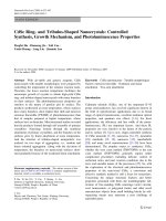
Figure 1: Two-step process to track individuals. (A) Source separa-
tion. (B) Tracking and identification.
influence and improve the course of a discussion. For exam-

ple, a message could indicate when a maximal speech dura-
tion threshold has b een reached, or a teacher could be in-
formed that he/she has been speaking the majority of the
time.
If a system has to be effective outside of the especially
equipped rooms, it has to cope with conversational speech.
Investigations by Shriberg et al. [15] showed that overlap
is an important, inherent characteristic of conversational
speech that should not be ignored. Also, participants may
move more freely during a conversation. Equally, the envi-
ronmental parameter may change, for example, room trans-
fer function. A mobile system must be capable of adjusting
to these parameter changes.
We opted to use two microphones as they can be unob-
trusively integrated into clothing and mobile dev ices and as
we seek to replicate the human ability to locate audio sources
with two ears. The clothing has to be designed in such a way
that the relative position of the two microphones does not
vary due to movements. Additionally, a rotation sensor is re-
quired to compensate the changes of body orientation—the
compensation will be integrated during further algorithm
development. Employing a mobile device, the requirements
of the microphone position can be easier satisfied as the
microphone spacing is fixed and the mobile device can be
placed on the table.
The audio data is recorded as a stereo audio st ream, for
example, each of the two microphones is recorded as one of
the two stereo channels. The stereo audio stream is treated
in the two-step process shown in Figure 1. First, the audio
data is separated into individual audio streams for each de-

tected source, respectively, speaker (A); then for each of these
streams, individuals are tracked and identified (B). Step (B)
may support step (A) by providing a feedback, for example,
by providing information as to which location of an individ-
ual can be expected. Also, the location information (step (A))
can be used to bias the identifier (step (B)), for example, the
individuals in the speaker database may not have an equal a
priori probability.
To c ompar e d ifferent system configurations, we intro-
duce a benchmark methodology. This benchmark is based on
performance metrics for each of the two steps ((A) and (B)).
We apply the concept of recall and precision [16]asametrics
to measure the system accuracy. Given that we target a mo-
bile system, we also introduce a complexity factor that is pro-
portional to the use of computational resources as metrics
to measure the system energy consumption. The benchmark
metrics and the system performance are evaluated with ex-
periments in an office environment. The experiments point
out the influence of microphone spacing, time frame dura-
tion, overlap of time frames, and sampling frequency.
Thenoveltyofthispapercanbefoundinanumberof
areas. Firstly, a system is presented that combines speaker
separation and tracking. In particular, a feedback loop be-
tween speaker separation and speaker tracking is introduced
and optimal system parameters are determined. Secondly,
the system addresses the speaker tracking problem with over-
lap between different sound sources. Thirdly, a mobile sys-
tem is targeted, for example, only limited system resources
are available and the acoustical parameters are dynamic. Fi-
nally, a novel benchmark methodolog y is proposed and used

to evaluate accuracy and computation complexity. Compu-
tation complexity has not been previously used as a design
constraint for speaker separation and tracking systems.
A description of the implemented system and of the
three tuning parameters is given in Section 2.InSection 3,
we present the benchmark methodology for the two-step
speaker separation and tracking system. The experimental
setup and simulation results are presented in Section 4. These
show that recall and precision of the separ a tion are indepen-
dent of sampling frequency, but depend on the time frame
duration. We also show that the feedback loop improves re-
call and precision of the separation step (step (A)).
2. SYSTEM DESCRIPTION
In this section, we present our implementation of the two-
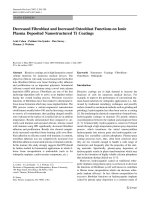
step system shown in Figure 1. The complete signal flow
in Figure 2 includes a preprocessing step. The preprocess-
ing step reduces signal noise and enhances the higher spec-
trum components to improve speaker recognition perfor-
mance. A bandpass filter ([75 7000] Hz) and preemphasize
filter (1
− .97z
−1
) are applied to each of the two input audio
streams. In the first processing step (A) the different audio
sources are separated. The implemented blind source sepa-
ration (BSS) algorithm is based on spatial cues. The audio
data having the same spatial cues are clustered to an audio
stream. In the second step (B), indiv iduals are tracked and
identified for each audio stream. To each individual audio
stream three tasks are applied. First, the audio stream is split

into speech and nonspeech frames. Then the speech frames
are analyzed for speaker changes. Lastly, the data between two
speaker change points and/or between speech bounds is used
to identify a speaker.
2.1. Blind source separation (step (A))
A source separation algorithm has to fulfill the following two
criteria to be suitable for our proposed system. First, the al-
gorithm has to cope with more sources than sensors. The
U. Anliker et al. 3
s1(t)
s2(t)
f 1(t)
Filter
Filter
Source
separation
(step A)
Speech-location
Speaker tracking (step B)
Segmentation
speech/nonspeech
Speaker change
detection
Speaker
identification
Figure 2: Data flow: the input data stream s1( t)ands2(t) is first filtered. A BSS algorithm splits the input stream into a data stream for
each active audio source based on spatial cues (step (A)). Step (B): for each source location the data is segmented in speech and nonspeech
segment. The speech segments are analyzed for speaker changes and later a speaker identity is assigned.
separation problem is degenerated and traditional matrix in-
version demixing methods cannot be applied. Second, the

system has to provide an online feedback to the user. The
algorithm has to be capable of separating the data and pro-
ducing an output for each audio source for every time seg-
ment. The sound source location can be employed to clus-
ter the audio data and to bias the speaker identifier. There-
fore, algorithms that provide location information directly
are favored. The degenerate unmixing estimation technique
(DUET) algorithm [17] fulfills the above cr iteria. The algo-
rithm performance is comparable to other established blind
source separation (BSS) methods [18]. One of the separation
parameters is the time difference of arrival (TDOA) between
the two microphones. We give a description of the DUET al-
gorithm and introduce two of our modifications.
The input signal is a stereo recording of an audio scene
(X
1
(t)andX
2
(t)). The input data stream is split into over-
lapping time frames. For each time frame the short time
Fourier transformation (STFT) for both channels, X
1
[k, l]
and X
2
[k, l], is computed. Based on the STFT, the phase delay
˜
δ[k, l] =−
m
2πk

∠
X
2
[k, l]
X
1
[k, l]
(1)
and the amplitude ratio
˜
α[k, t]
=





X
2
[k, l]
X
1
[k, l]





(2)
between the two channels are calculated. m is the STFT

length, k the frequency index, and l the time index. ∠ de-
notes the argument of the complex number. The data of a
particular source has a similar phase delay and amplitude ra-
tio.
The time frames are grouped into t ime segments. For
each time segment, that is, the frame group, a 2D histogram
is built. One direction represents the amplitude ratio and the
other the phase delay. We expect that the bins of the 2D his-
togram corresponding to a phase delay and an amplitude
ratio of one source will have more data points and/or sig-
nal energy than others. Thus, each local maximum in the
histogram represents an audio source. Each (
˜
δ[k, i],
˜
α[k, i])-
data point is assigned to one of the local maximums, that
is, source, by a maximum likelihood (ML) estimation. The
algorithm assumes that the sources are pairwise W-disjoint
orthogonal, that is, each time-frequency point is occupied by
one source only. The W-disjoint orthogonality is fulfilled by
speech mixtures insofar as the mixing parameter can be esti-
mated and the sources can be separated [19].
Our first experiments demonstrated two issues. First, in
the presence of reverberation (e.g., as in office rooms) the
performance of the DUET algorithm degenerates. Second, if
the two microphones are placed close together—compared
to the distance between the sources and the microphones—
the amplitude ratio is not a reliable separation parameter. To
address these two issues, the DUET algorithm is modified.

First, a 400-bin 1D histogram based on
˜
δ[k, i]isemployed.
The histogram span is evenly distributed over twice the range
of physical possible delay values. The span is wider than
the physical range as some estimations are expected to be
outside the physical range. Second, the implementation uses
the number of points in each bin and not a power-weighted
histogram as suggested in [17]. Data points which lie in a
specified frequency band are considered, see next paragraph.
To reduce the influence of noise, only data points that have a
total power of 95% of the frequency band power in one time
segment are taken into account. We refer to this modified
DUET implementation as DUET-PHAT (phase transform).
The modifications are deduced from the single-source case.
For a single-source TDOA estimation by generalized cross
correlation (GCC), several spectral weighting functions have
been proposed. Investigation on uniform cross-correlation
(UCC), ML, and PHAT time-delay estimation by Aarabi et
al. [20] showed that, overall, the PHAT technique outper-
formed the other techniques in TDOA estimation accuracy
in an office environment.
Basu et al.[21] and others showed that the full signal
bandwidth cannot be used to estimate the delay between two
microphones. The phase shift between the two input sig-
nals needs to be smaller than
±π. If signal components ex-
ist that have a shorter signal period than twice the maximal
4 EURASIP Journal on Applied Signal Processing
delay, bigger phase shifts can occur and the BSS results are

no longer reliable. For our configuration (microphone spac-
ing of 10 cm) this minimal signal period is 0.059 millisecond,
which is equivalent to a maximal frequency f
crit
of 1.7 kHz.
Increasing the low-pass filter frequency above 1.7 kHz has
two effects. Firstly, the delay accuracy in the front region
(small delay) is increased. Secondly, delay a ccuracy at the
sides is reduced, see Section 4.1.2. We decided to use a [200
3400] Hz digital bandpass filter for the blind source sep-
aration step for two reasons. First, the maximum energy
of average long-term speech spectrum (talking over one
minute) lies in the 250 Hz and the 500 Hz band. Second,
we expect most individuals to be in front of the micro-
phones.
If speakers and/or the system moves, the mixing parame-
ters will change. To cope with dynamic parameters, the time
segments have to be short. Our experiments showed that a
time segment duration of t
seg
= 1.024 seconds is suitable
to separate sources as recall is above 0.85; for information
t
seg
= 0.512 second has a recall of 0.50. The identification
trustworthiness is correlated to the amount of speaker data.
To increase the speaker data size our algorithm tracks the
speaker location. If the speaker location has changed less than
dis
max

= 0.045 millisecond since the last segment, we assume
that the algorithm has detected the same speaker. Therefore,
a speaker moving steady-going from the left side (view an-
gle
−90 degrees) to the right side (view angle +90 degrees)
in 20 seconds can be theoretically followed. Our experiments
showed a successful tracking if the speaker took 60 seconds
or more.
2.2. Speaker tracking (step (B))
The data with similar delay and thus with similar location are
clustered into one data stream. Each stream can be thought
of as a broadcasting channel without any overlaps. Systems
to detect speaker changes and to identify the speakers have
been presented by several research groups, see [5–7, 22]. In
the next paragraphs, we present our implementation.
The audio data is converted to 12 MFCCs (mel-frequency
cepstrum coefficients) and their deltas. The MFCCs are cal-
culated for each time frame. The annotation of the au-
dio stream is split into three subtasks. First, the audio
stream is split into speech and nonspeech segments. Sec-
ond, the speech segments are analyzed for speaker changes.
An individual speaker utterance is then the data between
two speaker change points and/or between speech segment
bounds. Third, the speaker identity of an individual utter-
ance is determined, that is, the data from a single utterance is
employed to calculate the probability that a particular per-
son spoke. If the normalized probability is above a preset
threshold, then the utterance is assigned to the speaker with
the highest probability. If the maximum is below the thresh-
old, a new speaker model is trained. Overall, the speaker

tracking algorithm extracts time, duration, and the num-
ber of utterances of individual speakers. Intermediate re-
sults can be shown or recorded after each speaker utter-
ance.
2.2.1. Speech/nonspeech detection
Only data segments that are comprised mainly of speech can
be used for identifying an individual speaker. Nonspeech seg-
ments are therefore excluded. The most commonly used fea-
tures for speech/nonspeech segmentation are zero-crossing
rate and short-time energy, for example, see [23]. The in-
put data is separated and clustered in the frequency domain.
Thus, it is computationally advantageous to use frequency
domain features to classify the frames. Spectral fluctuation
is employed to distinguish between speech and nonspeech.
Peltonen et al. used this feature for computational auditory
scene analysis [24] and Scheirer and Slaney for speech-music
discrimination [25].
2.2.2. Speaker change
The goal of the speaker change detection algorithm is to ex-
tract speech segments, during which a single individual is
speaking, that is, split the data into individual speaker ut-
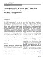
terances. The signal flow of the speaker change detection
algorithm is shown in Figure 3. The algorithm is applied
to the speech data of an utterance, that is, the nonspeech
data is removed from the data set. If for more than t
pause
=
5 seconds nonspeech segments are detected or if for more
than t
speaking

= 15 s an utterance is going on, then the speaker
change detection and identification is executed. To reduce the
influence of the recording channel, CMS (cepstral mean sub-
straction) [26] is applied.
Depending on the data size, two different calculation
paths are taken. If the speech data size is smaller than t
1
=
2.048 seconds, the data is compared to the last speech seg-
ment. The two data sets are compared by the Bayesian infor-
mation criterion (BIC) [27]:
Δbic
=−
n
1
2
log det(C
1
) −
n
2
2
log det(C
2
)
+
n
2
log det(C)+λ
· p,

p
=
1
2

d +
d(d +1)
2

log(n),
(3)
where n
1
and n
2
are the data size of first and second data seg-
ment, respectively, the overall data size n
= n
1
+ n
2
. C, C
1
,
and C
2
are the diagonal covariance matrix estimated on the
data set. d is the data dimensionality. λ is the penalty weight,
we use 1. If the Δbic value is above zero, this means that no
speaker change occurred and the speech segment is given the

same speaker identification as the last one. If Δbic is below
zero, then a speaker change is assumed and the speaker iden-
tificationmoduleiscalled.
For long speech segments, the algorithm checks for inter-
nal speaker changes. The speaker change detection has three
sequential processes with each confirming the findings of the
previous process. The first process is based on the compar-
ison of two adjacent segments of t
1
/2 duration. A potential
speaker change p oint is equal to the local maximum of the
distance measure D. The data segments are represented by a
U. Anliker et al. 5
Speech/nonspeech
Speech data
Segment >t
1
BIC
Same speaker
No identifictation
BIC < 0
Segment >t
2
Calc. distance
Local maximum
End of segement
BIC
BIC < 0
Speaker identification
Yes

Yes
Yes
Yes
Yes
No
No
No
No
No
Figure 3: Speaker change detection: for short segments a speaker identification is performed directly. Long speaker segments are checked
for intra speaker changes. Consequently, the identifier is run on homogeneous data segments.
unimodal Gaussian mixture with diagonal covariance matrix
C. The distance D is calculated by [7]
D(i, j)
=
1
2
tr

C
i
− C
j

C
i
−1
− C
j
−1


,(4)
tr is the matrix trace. A potential speaker change is found
between ith and (i+1)th segment, if the following conditions
are satisfied: D(i, i+1) >D(i+1, i+2), D(i, i+1) >D(i
−1, i),
and D(i, i+1) >th
i
,whereth
i
is a threshold. The threshold is
automatically set according to the previous s
= 4 successive
distances:
th
i
= α
1
s
s

n=0
D(i − n − 1, i − n), (5)
α is set to 1.2. The segment is moved by 0.256 second. This is
equivalent to the speaker change resolution.
The second process validates the potential speaker
changes by the Bayesian information criterion (BIC), for ex-
ample, as in [28–30]. If the speaker change is confirmed
or the end of the speech segment is reached, the utterance
speaker is identified.

In the third process of the speaker change detection the
speaker identification can be seen. The implementation is de-
scribed in the next sect ion. For two adjacent utterances the
same speaker can be retrieved. Only if a speaker change is
confirmed by all three processes a new sp eaker is retrieved.
2.2.3. Speaker identification
A speaker identification system overview including the
recognition performance can be found in [31]. For conver-
sational speech, the speaker identifier has to deal with short
speech segments, unknown speaker identities (i.e., no pre-
training of the speaker model is possible), unlimited number
of speakers (i.e., the upper limit is not known beforehand),
and has to provide online feedback (i.e., the algorithm can-
not work iteratively). We have implemented an algorithm
based on a world model, which is adjusted for individual
speakers.
The individual speakers are represented by a Gaussian
mixture model (GMM) employing 16 Gaussians having a di-
agonal covariance matrix. We employ 16 Gaussians as inves-
tigation by [32–34] showed that starting from 16 mixtures
a good performance is possible, even if only few feature sets
can be used to t rain the speaker model. The model input fea-
tures are 12 MFCCs and their deltas.
To identify the speaker of a speech utterance, the algo-
rithm calculates the log likelihood of the utterance data for
all stored speaker models. All likelihoods are normalized by
a world model log likelihood and by the speech segment du-
ration. If the normalized likelihoods (Λ)areaboveaprede-
fined threshold th
like

, then the speech segment is assigned to
the model with the maximum likelihood [35]:

(X) =
log p

X | λ
speaker

−
log p

X | λ
world

n
seg
,(6)
X is the input data, λ
speaker
the speaker model, λ
world
the
world model, and n
seg
the number of time frames. If the like-
lihoods are below the threshold, then a new speaker model is
trained using the world model as a seed for the EM (expecta-
tion maximization) algorithm.
6 EURASIP Journal on Applied Signal Processing

2.3. Feedback speech segments to BSS
Based on the speech/nonspeech classification, it is know n at
which location (represented by the delay) an individual is
talking. If at the end of a time segment an individual is talk-
ing (for each time segments the audio sources are separated),
then in the next time segment it is expected to detect an in-
dividual at the same location (expected locations).
The DUET-PHAT algorithm detects active sources, that
is, speakers, as local maximums in the delay histogram (de-
tected locations), see Section 2.1 . All speakers cannot be de-
tected in every segment, as the delay of a speaker can be
spread, for example, by movements or noise, or as the local
maximum is covered by a higher maximum.
The feedback loop between speaker tracking and BSS
compares the detected locations by the BSS and the expected
locations. A correspondence between expected and detected
locations is found, if the difference between the two delays is
smaller than dis
max
. If no correspondence for an expected lo-
cation is found, the delay is added to the detected locations.
The data points are assigned to one of the detected delays or
to the added delays by an ML estimation as without the feed-
back loop.
2.4. Parameters
Our two-step speaker separation and tracking system is con-
trolled by more than 20 parameters. Most of them influence
only a small part of the system, but if they are set incorrectly,
the data for the follow ing processing step is useless. The val-
ues used are mentioned in the text. The influences of the fol-

lowing four parameters are investigated one at a time in the
experiment in Section 4, keeping all other parameters con-
stant.
2.4.1. Microphone spacing
Placing the two microphones close together gives a high sig-
nal bandwidth which can be employed to estimate the source
location, see Section 2.1. On the other hand, the require-
ments on the delay estimation precision are increased.
2.4.2. Time frame duration
For each time frame the STFT is calculated. Low frequency
signals do not have a complete period within a short time
frame, which leads to disturbance. It is then not possible to
calculate a reliable phase estimation. The upper bound of the
time frame duration is given by the assumption of quasista-
tionary speech. The assumption is fulfilled up to several tens
of milliseconds and fails for more than 100 milliseconds [36].
Thetimeframeduration(t
frame
) determines the frequency
resolution ( f
res
):
f
res
=
f
sample
m
=
f

sample
f
sample
t
frame
=
1
t
frame
,(7)
where f
sample
is the sampling frequency and m the num-
ber of points in the STFT. Investigations by Aoki et al. [37]
showed that a frequency resolution between 10 and 20 Hz is
suitable to segregate speech signals. The percentage of fre-
quency components that accumulate 80% of the total power
is then minimal. Aoki et al. showed that for a frequency res-
olution of 10 Hz, the overlap between different speech sig-
nals is minimal. Baeck and Z
¨
olzer [38] showed that the W-
disjoint orthogonality is maximal for a 4096-point STFT,
when using 44.1 kHz sampling frequency, which is equiva-
lent to a f requency resolution of 10.77 Hz. We expect to get
best separation results for a time frame duration between
50 milliseconds and 100 milliseconds. The time frame dura-
tion typically used in sp eech processing is shorter. The dura-
tion is in the range of 10 milliseconds to 30 milliseconds.
2.4.3. Time frame shift

The t ime frame shift defines to what extent the time frame
segments overlap. If the shift is small, more data is available
to train a speaker model and more time-frequency points can
be used to estimate the source position. However, the com-
putation complexity is increased.
2.4.4. Sampling frequency
The delay estimation resolution is proportional to the sam-
pling frequency. Increasing the sampling frequency increases
the computation complexity.
3. BENCHMARK
As we have a two-step system (Figure 1)weoptedforatwo-
step benchmark methodology; a further reason for such an
approach is that the performance of step (B) depends on the
performanceofstep(A).
In designing the benchmark, the following two cases have
to be taken into account. The first is that only sources de-
tected during the separation step can be later identified as in-
dividuals. The second issue is that if too many sources are de-
tected, three different outcomes are possible. In the first out-
come, a noise source is detected which can be eliminated by a
speech/nonspeech discriminator. In the second outcome, an
echo is detected, which will be considered as separate indi-
vidual or the identification allows the retrieval of the same
individual several times in the same time segment, then a
merging of these two to one is possible. In the third outcome,
depending on the room transfer function and noise, nonex-
istent artificial sources can be retrieved that will collect signal
energy from the true sources. These outcomes will impact the
performance of the identification step.
In order to cope with the dependance between the two

steps, the system is first benchmarked for step (A) and then
for both steps (A and B) including the feedback loop (B
→ A).
For both steps, we define an accuracy measure to quantify
the system performance. The measures are based on recall
and precision. Ground t ruth is obtained during the exper i-
ments by a data logger that records the start and stop time of
a speech utterance and the speaker location.
U. Anliker et al. 7
As mobile and wearable systems usually run on batter-
ies, a strict power budget must be adhered to. During system
design, different architectures have to be evaluated with the
power budget in mind. Configurations that consume less sys-
tem resources are favored. A second optimization criterion
deals with the system power consumption. During the algo-
rithm development, we assume a fixed hardware configura-
tion. The energy consumption is therefore proportional to
the algorithm complexity. We introduce a relative complexity
measure which reflects the order and ratio of the computa-
tion complexity.
3.1. Accuracy
We introduce for step (A) an accuracy metrics which reflects
how well sound sources have been detected. The overall sys-
tem metrics reflects how well individual speakers are identi-
fied and tracked. We selected an information retrieval accu-
racy metrics [16] as this metrics is calculated independently
of the number of sources, is intuitive, and the ground truth
can be recorded online.
3.1.1. Step (A)
The implemented separation algorithm estimates for each

segment and each source the signal delay between the two
microphones. The delay estimation is defined as correct if the
difference between the true delay and estimated one is below
a preset tolerance.
Recall (rec) is defined as the number of segments in
which the delay is estimated within a preset tolerance to the
ground truth divided by the total number of active segments
of the source. If more than one source is active, then the min-
imal recall rate is of interest. For example, if two sources are
active, one source is detected correctly and the second one
not at all, the average recall rate is 0.5 and the minimum 0.0.
The signal of the second source is then erroneously assigned
to the detected one. Indeed, the audio data is not separated.
The speaker identification has to be accomplished with over-
lapping speech, which is not possible.
Precision (pre) is defined as the number of correctly es-
timated delays (difference between the estimation and the
ground truth is smaller than a preset tolerance) div ided by
the total number of retrieved delay estimations. An over-
all precision is calculated. In the multisource case, retrieved
delays may belong to any of the active sources. Estimations
which differ more than the preset tolerance to any source are
considered as er roneous.
Precision and recall values are combined into a single
metrics using the F-measure. The F-measure is defined as
[39]
f
= 2
rec
· pre

rec + pre
. (8)
To summarize, recall is equal to one if in all time seg-
ments all sources have been detected. If no sources are de-
tected, then recall is zero. Precision is unity if no sources
are inserted, and decreases towards zero as more nonexisting
Table 1: Definition of the confusion matrix for our experiments:
rows represent the ground truth speaker and columns the retrieved
speakers. SP R
i
is the ith retrieved speaker, and SP T
j
is the jth
ground truth speaker.
Ground truth Speaker retrieved
speaker
SP R
1
SP R
n
SP T
1
SP R
1
when SP T
1
Duration of SP T
1

SP R

n
when SP T
1
Duration of SP T
1
.
.
.
.
.
.
SP T
m
SP R
1
when SP T
m
Duration of SP T
m

SP R
n
when SP T
m
Duration of SP T
m
sources are detected. For a flawless working system, recall and
precision are equal to one. If many nonexisting sources are
inserted, precision is low and the signal energy is distributed
among the inserted sources. None of the sources will repre-

sent a speaker as the speaker features are split between the
erroneously detected audio sources. The speaker identifica-
tion cannot identify any speaker reliably. If many sources are
not detected, recall is low and the signal energy is linked to
a wrong source. The speaker features of two or more speak-
ers are then combined to one. Possibly the dominant speaker
might be detected, that is, the speaker with the highest sig nal
energy, or a new speaker is retrieved.
3.1.2. Step A + B
This system accuracy metrics has to reflect how well indi-
vidual speakers are identified and tracked. We compare time
segments assigned to one individual with the ground truth.
Thesystemrecall(rec
sys
)isdefinedasthedurationofcor-
rectly assigned speech segments div ided by the total duration
of the speech. If for one time segment several speakers are re-
trieved, then the segment is counted as correct if the speaker
has been retrieved at least once.
The system false rate (fal
sys
) is the duration of data which
has been assigned erroneously to one speaker divided by the
total retrieved speech dur ation. If in one time segment the
correct speaker has been retrieved more than once, the time
for the second retrieval is also considered to be assigned cor-
rectly, that is, we allow the same speaker to be at different
locations in one time segment. The system is not penalized
for detecting echoes.
To get a deeper insight of the system accuracy, we in-

troduce a confusion matrix, see Table 1. Rows represent the
speaker ground truth. Each column represents a retrieved
speaker. It is possible for more or less speakers to be re-
trieved than there are ground truth speakers since the num-
ber of speakers is determined online by the algorithm. For
each ground truth speaker (row), the time assigned to a re-
trie ved speaker (column) is extracted and then divided by
the total speech time of the ground truth. The correspon-
dence between retrieved speaker and ground truth speaker
is calculated as follows: the maximal matrix entry (retrieved
speaker time) is the first correspondence between ground
truth (row index) and retrieved speaker (column index). Row
and column of this maximum are removed from the matrix.
The next correspondence is the maximal matrix entry of the
8 EURASIP Journal on Applied Signal Processing
Table 2: Sampling frequency complexity factor.
Frequency Application Factor
08 kHz Telephone line 1
16 kHz
Video conference, G.772 2
22.05 kHz
Radio 2.76
32 kHz
Digital r adio 4
44.1 kHz
CD 5.51
Table 3: Approximation of the STFT complexity factor.
No. of points Factor
128 1
256 0.75

512 0.62
1024 0.56
2048 0.53
4096 0.52
remaining matrix. These steps are repeated until the matrix
is empty.
3.2. Computation complexity
During the algorithm optimization, we assume that the hard-
ware configuration is fixed. The energy consumption is then
proportional to the computation load. The computation
load can be defined in terms of elementary operations or
classes of elementary operations as in [40]. If complex algo-
rithms are developed in a high-level environment, such as
Matlab, then it is a nontrivial task to estimate the number of
elementary operations. Furthermore, during development it
is not e ssential to know the absolute values, for example, run
time, as these depend on the computation platform and on
the optimization techniques applied. To guide a design de-
cision, it is sufficient to know the order of the computation
load and the relation between the system variants, that is, the
ratio of the two run times. The computation complexity met-
rics has to provide the correct ranking and correct propor-
tionality of the computation load for the different parameter
settings.
We compare the computation complexity between dif-
ferent configurations for the same data set. We assume, if
the same data set is processed, then the same number of
speaker models is trained, and then the same number of
speaker probabilities is calculated. We assume further that
the training time and likelihood calculation t ime increases

linearly with the size of the data. The computation complex-
ity is influenced by the following evaluated parameters: sam-
pling frequency, time frame duration, and overlap of time
frames. We introduce for each parameter a complexity fac-
tor. To calculate the overall design choice relative computa-
tion complexity the product of sampling frequency complexity
factor, STFT complexit y factor,andoverlap complexity factor
is taken.
The computation complexity is proportional to the sam-
pling frequency. We define the sampling frequency complex-
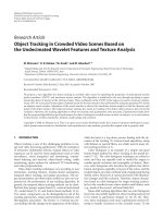
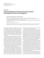
−30 degrees
0degrees
15 degrees
30 degrees
45 degrees
60 degrees
85 degrees
Microphone 1 Microphone 2
Figure 4: Microphone configuration and source directions.
ity factor for 8 kHz a s 1 and increase it proportionally to the
sampling frequency, see Table 2.
The STFT complexity factor is defined as a weighted sum
of the relative change of the number of processed data points
plus the relative change of the processed time frames. As a
first approximation, we set the weight for both to 0.5. The
resulting STFT complexity factor can be found in Ta ble 3.
The overlap complex ity factor issetto1whennoover-
lapping occurs. If the time frames overlap by 50%, then the
number of frames and data points to process are doubled and
the factor is set to 2. If the time frames overlap by 75%, the

factor is set to 4. If the time frames overlap by 85.5%, the
factor is set to 8.
4. EXPERIMENTS AND RESULTS
We employ the experiments to show that the accuracy and
relative computation complexity metrics int roduced can be
used to benchmark a two-step speaker separ ation and track-
ing system and to validate our system design. The experi-
ments are based on 1 to 3 persons talking at fixed locations.
The recordings are made in an office environment. Two mi-
crophones are placed on a table. A loudspeaker is placed 1m
away in front of the microphones. For the single-source ex-
periment the loudspeaker is placed at 0, 15, 30, 45, 60, 85
degrees angles to the microphone axis, see Figure 4. For the
two-source experiment one loudspeaker was placed at 0 de-
grees and a second one at 30 degrees. For the three-source
experiment one additional loudspeaker is placed at
−30 de-
grees. The distance between the two microphones is 10 cm, if
not otherwise stated.
4.1. Phase delay estimation (step (A))
We compare delay estimations of DUET-PHAT, the GCC-
PHAT (GCC employing PHAT spectral weighting function),
and the original DUET [17] algorithm. In the multisource
case, we do not consider the GCC-PHAT estimations. We
calculate the delay estimation distribution for each of the 6
U. Anliker et al. 9
0.10−0.1−0.2−0.3−0.4−0.5−0.6
Phase delay (ms)
0.01
0.02

0.03
0.04
0.05
0.06
0.07
0.08
0.09
Probability
32 kHz sampling frequency (2048 point FFT)
0degrees(0ms)
15 degrees (0.16 ms)
30 degrees (0.31 ms)
45 degrees (0.45 ms)
60 degrees (0.54 ms)
85 degrees (0.63 ms)
Figure 5: Smoothed probability distribution of the GCC-PHAT
TDOA estimation. The microphone spacing is 20 cm. The input sig-
nal is sampled at 32 kHz, and the microphone spacing is 20 cm. The
STFT length is 2048 points.
locations and for each sampling frequency and for each STFT
length.
4.1.1. GCC-PHAT
The evaluation of the GCC-PHAT TDOA estimation showed
four properties. First, the maximum of the TDOA estima-
tion distribution is similar for the same time frame du-
ration (e.g., 8 kHz[sampling frequency]/512[STFT length],
16 kHz/1024 and 32 kHz/2048). Second, if the time frame
duration is kept constant and the sampling frequency in-
creases, the distribution gets narrower. Third, until a min-
imum time frame duration level is attained, that is, below

64 mil liseconds for the selected configuration, the maximum
of the distribution increases towards the true delay. Above
this minimal time frame duration, the distribution maxi-
mum is constant. Fourth, Figure 5 shows that the distribu-
tion variance increases and that the difference between the
true delay and the maximum of the distribution increases
with the delay. Starting from 45 degrees, the difference is
bigger than 0.05 millisecond. For our further evaluation, the
GCC-PHAT delay estimation is employed as a reference.
Based on the variance of the GCC-PHAT estimation, we set
the tolerance to 0.025 millisecond for a 10 cm microphone
spacing.
4.1.2. Comparing GCC-PHAT, DUET, DUET-PHAT
Figure 6 shows the F-measure of GCC-PHAT, DUET, and
DUET-PHAT using two different low-pass cutoff frequencies
0.30.20.10
Expected delay (ms) 2 sources 3 sources
0
0.1
0.2
0.3
0.4
0.5
0.6
0.7
0.8
0.9
1
F-measure
Accuracy at 32 kHz

GCC-PHAT 1700 Hz
GCC-PHAT 3400 Hz
DUET 1700 Hz
DUET 3400 Hz
DUET-PHAT 1700 Hz
DUET-PHAT 3400 Hz
Figure 6: F-measure for the three different delay estimation al-
gorithms. High-pass cutoff frequency 200 Hz. Low-pass cutoff fre-
quency is 1700 Hz/3400 Hz. Plotted are 6 delay locations and two
multispeaker streams.
(1700 Hz [ f
crit
] and 3400 Hz [2x f
crit
]) and a high-pass cut-
off frequency of 200 Hz. The GCC-PHAT algorithm includes
checks to ensure that only reliable TDOA estimations are re-
ported. Consequently, whilst precision is high, recall is re-
duced.
For all approaches the accuracy declines with an in-
creasing delay/angle and number of simultaneous sources. If
the low-pass cutoff frequency is increased from 1700 Hz to
3400 Hz, the GCC-PHAT and DUET-PHAT F-measure in-
creases by at least 75%. The two implementations benefit
from the higher signal bandwidth as the spectral energy is
normalized. The DUET algorithm is not affected as the signal
energy is employed and as speech is expected to have maxi-
mum signal energy in the 250 Hz to 500 Hz band.
A comparison of the three implementations shows that
DUET is best for small view angles but declines faster than

the other two. DUET-PHAT is better than GCC-PHAT.
For three simultaneous sources only DUET-PHAT has a F-
measure above 0.3.
We decided to employ the DUET-PHAT implementation
as the performance is best in the multi-source scenarios. The
F-measure declines also slower than for the DUET imple-
mentation, if the true delay increases (view angle).
4.1.3. Microphone spacing
A microphone spacing of 5 cm, 10 cm, and 20 cm was eval-
uated. Reducing the microphone spacing increases f
crit
and
consequently a higher signal bandwidth can be employed to
estimate the source location. As the DUET-PHAT algorithm
10 EURASIP Journal on Applied Sig nal Processing
300250200150100500
Time frame duration (ms)
0.1
0.2
0.3
0.4
0.5
0.6
0.7
0.8
F-measure
Accuracy
8kHz
16 kHz
22.05 kHz

32 kHz
44.1kHz
Figure 7: F-measure evaluated for 5 different sampling frequencies
(8 kHz (
×), 16 kHz ( +), 22.05 kHz (◦), 32 kHz (), and 44.1 kHz
()) and a STFT length of 128, 256, 512, 1024, 2048, and 4096
points. x-axis is STFT length in ms.
profits from a higher signal bandwidth, 5 cm showed best
single-source accuracy followed by 10 cm and 20 cm. In the
multisource case a 5 cm spacing cannot separate more than
two sources. 10 cm spacing shows best F-measure for two
sources but a reduced value for three simultaneous sources
compared to 20 cm.
If the microphone spacing is reduced, the maximal de-
lay values are reduced proportionally and small estimation
fluctuations have a higher influence. In the single-source case
these fluctuations are averaged as the number of data points
is high. In the multisource case, the second or third source
cannot be extracted as local maximum anymore. The sources
are seen only as a small tip in the slope towards the global
maximum, which could also be from noise.
The microphone spacing is therefore a tradeoff between
signal bandwidth and delay estimation accuracy. The delay
estimation accuracy is influenced, for example, by micro-
phone noise and variation of the microphone spacing. The
change of the delay by spacing variation has to be small com-
pared to variations due to movements. For a microphone
spacing of 10 cm a change by 0.5 cm is acceptable as similar
changes by noise are observed.
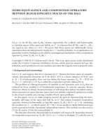
4.1.4. Time frame duration

Figure 7 shows the F-measure for the speakers talking con-
tinuously at 30 degrees (0.15 millisecond) and for three
simultaneous sources. The time frame duration is varied
from 3 milliseconds (44.1 kHz/128 point STFT) to 510 milli-
seconds (8 kHz/4096 point STFT, 32 kHz/16384).
In the single-source case, if the time frame-duration in-
creases, the F-measure increases. In the multisource case,
the F-measure maximum lies between 60 milliseconds and
130 milliseconds. Except for 8 kHz, where the maximum is at
256 milliseconds. The F-measure differs less then 3 percent
compared to that measured at 128 milliseconds. The plotted
F-measure is calculated with the minimal recall rate. If the
average recall is considered, the maximum is moved towards
longer time frame duration, the drop after the maximum is
slower and the ascending slope of the F-measure is similar to
the plotted one.
Time fr ame duration is a tradeoff between BSS accuracy
and the assumption of speech quasistationarity. Blind source
separation favors a time frame duration of 60 millisecods
or longer. Aoki et al. [37] and Baeck and Z
¨
olzer. [38]pre-
sented best source separation for 100 milliseconds (maximal
W-disjoint orthogonality). On the other hand, in speech pro-
cessing time frame durations of 30 milliseconds or below are
typically employed.
Therefore, we decided to employ a time frame dura-
tion of 64 milliseconds for 8 kHz, 16 kHz, and 32 kHz and
93 milliseconds for 22.05 kHz and 44.1 kHz for our further
experiments. Our speaker tracking experiments and the lit-

erature [41] show that under these conditions the sources
can b e separated and the quasistationarity assumption is still
valid.
4.1.5. Time frame overlap
Tabl e 4 shows for two locations (15 degrees and 30 degrees)
and for three simultaneous sources that the time frame over-
lap has small influence on the location accuracy. The results
for the tested sampling frequencies, the tested locations, and
for simultaneous sources are similar to the one reported in
Tabl e 4 . A system which only extracts location information
would therefore be implemented with nonoverlap between
the time frames to minimize the computation load.
4.1.6. Sampling frequency
If the sampling frequency is changed, that is, the frame du-
ration and the overlap is kept constant, then the influence
on the delay estimation accuracy is small, see Figure 8.For
the source location detection we do not use the entire sig-
nal spectrum. Only signals in the frequency band 200 Hz
to 3400 Hz are considered. As the time frame duration is
equivalent to the frequency resolution, the number of points
in the frequency band is independent of the sampling fre-
quency and consequently the performance is similar. The
slightly higher F-measure for 22.05 kHz and 44.1 kHz is due
to the longer time segment.
4.1.7. Conclusions
To minimize computation load and maximize the perfor-
mance, a low sampling frequency, nonoverlapping time
frames, and a time frame duration between 50 milliseconds
and 100 milliseconds should be used. The relative complex-
ity is in the range from 0.62 (8 kHz, no-overlap) to 36.15

U. Anliker et al. 11
Table 4: The percentage gives the distance in which the time frame is moved. The values are recall/ precision.
100% 75% 50% 25% 12.5%
08 kHz, STFT 512, delay 0.08 ms  15
◦
0.82/0.82 0.83/0.81 0.81/0.80 0.82/0.82 0.81/0.80
16 kHz, STFT 1024, delay 0.08 ms  15
◦
0.81/0.81 0.83/0.83 0.81/0.81 0.82/0.81 0.81/0.81
08 kHz, STFT 512, delay 0.15 ms  30
◦
0.69/0.57 0.71/0.58 0.68/0.56 0.70/0.57 0.68/0.57
16 kHz, STFT 1024, delay 0.15 ms  30
◦
0.69/0.57 0.70/0.58 0.70/0.58 0.71/0.59 0.68/0.56
3 streams (
−0.15 ms/0.0 ms/0.15 ms) 8 kHz, STFT 512 0.22/0.69 0.22/0.71 0.26/0.68 0.23/0.69 0.23/0.70
3 streams (
−0.15 ms/0.0 ms/0.15 ms) 16 kHz, STFT 1024 0.21/0.70 0.22/0.70 0.25/0.67 0.22/0.69 0.22/0.69
0.30.20.10
Expected delay (ms) 2 sources 3 sources
0
0.1
0.2
0.3
0.4
0.5
0.6
0.7
0.8

0.9
F-measure
Accuracy
8 kHz, STFT 512
16 kHz, STFT 1024
22.05 kHz, STFT 2048
32 kHz, STFT 2048
44.1 kHz, STFT 4096
Figure 8: F-measure evaluated for constant time frame duration
and 5 different sampling frequencies.
(44.1 kHz, 12.5% time frame shift). This outcome reduces
the possible parameter combinations from 120 to 24 (80%
reduction).
4.2. Speaker tracking (step A + B)
The overall system performance is evaluated in two steps.
First, the improvement of the source separation by the feed-
back loop is shown. And second, system recall and false rate
are e valuated.
4.2.1. Influence of the feedback
Tabl e 5 shows recall and precision with and without feed-
back loop. In the single-source case, if the delay is be-
low 0.15 millisecond, then the BSS algorithm retrieves the
correct location for 75% or more of the time segments.
The feedback slightly increases the recall rate. Starting from
0.19 millisecond the BSS algorithm erroneously retrieves two
sources instead of one. Precision is roughly halved compared
to delays of 0.15 millisecond and below. Depending on the
input signal either one or both locations are retrieved. The
feedback adds the missed location to the estimation if the
last segment has been classified as speech. Adding missed lo-

cation increases the recall rate. The segment of the true lo-
cation is more often classified as speech than the other one,
this leads to increased precision. If no reliable source location
is possible as for 0.27 millisecond delay, the feedback cannot
improve the situation. In the multisource case the feedback
adds delays of speaker locations which have not been de-
tected and therefore recall is increased.
4.2.2. System recall and false rate
The evaluation of the blind source separation showed that
speakers are detected in up to 80% of the cases if one indi-
vidual is speaking and the view angle is smaller than 30 de-
grees. If the speakers are located at greater angles (more to
the side) recall rapidly deteriorates. In the multisource case
recall is about half of the single-source case. We first tested
if a human can distinguish between individual speakers. The
test subject observed that the filter process introduces a click-
ing noise and that acoustical changes are in some instances
abrupt.
Tabl e 6 reports the results for one speaker at 30 degrees
and Table 7 for two simultaneous speakers. System recall,
false rate, number of retrieved speakers, and th
like
for which
the results are achie ved are stated in the table. Two simultane-
ous speakers give a lower system recall and a higher false rate
than one speaker as the source separation introduce noise
and acoustical changes. For three simultaneous speakers no
speaker identification was possible due to interferences intro-
duced by the separation.
Highest system recall and lowest false rate is shown for

8 kHz sampling frequency. The performance difference be-
tween the sampling frequencies is significantly smaller for
other data sets. The 16 kHz sampling frequency accuracy is
similar to higher sampling frequencies as the input signal is
low-pass filtered at 7.5 kHz. For other experiments best accu-
racy has been observed for sampling frequencies other than
8 kHz.
For an autonomous system the threshold th
like
has to
be independent of the data set, experiment, and number of
speakers. T he experiments showed that the optimal thresh-
old differs between data sets and experiments. We also ob-
served an intraspeaker variability which leads in some in-
stances to far more retrieved speakers than there are in the
ground truth (e.g., 16 kHz, Ta ble 6).
12 EURASIP Journal on Applied Sig nal Processing
Table 5: Recall/ precision for different locations. 16 kHz sampling frequency. [200,3400] Hz bandpass. Step (A) does not include the knowl-
edge of previous separation steps. Feedback does include location into the BSS step which has been classified as active location.
0.00 ms  0
◦
0.08 ms  15
◦
0.15 ms  30
◦
0.19 ms  45
◦
0.23 ms  60
◦
0.27 ms  85

◦
Step (A) 0.82/0.84 0.77/0.77 0.73/0.62 0.59/0.35 0.33/0.23 0.01/0.01
Feedback 0.82/0.77 0.81/0.77 0.78/0.64 0.72/0.38 0.52/0.30 0.01/0.01
Results for 2 and 3 simultaneous sources
0 ms and 0.15 ms
−0.15 ms, 0 ms, and 0.15 ms
Step (A) 0.39/0.81 0.24/0.67
Feedback 0.45/0.81 0.30/0.67
Table 6: System recall and false rate. Location 0.15 ms  30 degrees, single source, 4 speakers (1 female, 3 males).
8 kHz/512 16 kHz/1024 22.05 kHz/2048 32 kHz/2048 44.1 kHz/4096
Recall 0.64 0.43 0.32 0.43 0.43
False rate 0.36 0.55 0.64 0.51 0.47
Number of speakers 3 15 6 16 11
th
like
18 7 8 10.5 10
Table 7: System recall and false rate. Two simultaneous sources, 4 speakers (2 females, 2 males).
8 kHz/512 16 kHz/1024 16 kHz/1024 22.05 kHz/2048 32 kHz/2048 44.1 kHz/4096
Recall 0.33 0.39 0.33 0.28 0.27 0.20
False rate 0.56 0.69 0.56 0.51 0.63 0.59
Number of speakers 5 5 3 10 10 6
th
like
12 7 4 8.5 8.5 3
Table 8: Speaker confusion matrix. Two females (SP T1, SP T3) and 2 males (SP T2, SP T4) ground truth speakers. Bold represents the
mapping between retrieved and true speakers.
8 kHz/512, delay 0.08 ms  15
◦
16 kHz/1024, 2 simultaneous sources
rec

sys
= 0.50, fal
sys
= 0.51, dis
th
= 18 rec
sys
= 0.39, fal
sys
= 0.69, dis
th
= 7
SP R1 SP R2 SP R3 SP R4 SP R1 SP R2 SP R3 SP R4 SP R5
SP T1 1.00 0.00 0.00 0.00 0.00 0.36 0.00 0.00 0.48
SP T2
0.27 0.52 0.10 0.10 0.00 0.05 0.00 0.04 0.80
SP T3
1.00 0.02 0.00 0.00 0.01 0.47 0.00 0.00 0.42
SP T4
0.88 0.00 0.00 0.00 0.00 0.27 0.00 0.05 0.63
4.2.3. Speaker confusion matrix
Tabl e 8 shows the confusion matrix for a single-source at 15
degrees and two simultaneous sources. In the single source
case mostly SP R1 is retrieved. For SP T2, 52% of the time SP
R2 is retrieved.
In the multisource case, mainly SP R2 and SP R5 are re-
trieved. The SP R2 and SP R5 are not assigned to one loca-
tion. SP R2 is retrieved for the first two minutes and SP R5
afterwards. To SP R1 and SP R3 only segments are assigned
which have in total less than 1% of the ground truth speak-

ing time. For the two simultaneous sources, the mapping be-
tween retrieved and ground truth speaker looks as follows:
SP T1–SP R2, SP T2–SP R5, SP T3–SP R1, and SP T4–SP R4.
4.2.4. Conclusion
A feedback from the speaker tracking step to the BSS im-
proves the location performance. The evaluation of the sys-
tem recall, system false rate, and speaker confusion matrix
showed that the identification step can be improved and the
parameter cannot be fixed at this stage. To improve the iden-
tification step, the clicking noise introduced by the filtering
process has to be reduced by means of incorporating sp eech
properties. Additionally, the three metrics have been shown
to be a valuable tool to judge the performance.
5. CONCLUSION
In this paper, we have presented a system that combines
speaker separation and tracking in a two-step algorithm. The
system addresses the speaker tracking problem also if over-
laps between different sound sources exist. The system has
been designed taking the constraints of a mobile environ-
ment into account, such as limited available system resources
and dynamic acoustical parameters.
Additionally, we proposed a novel benchmark methodol-
ogy to evaluate accuracy and computation complexity. Our
U. Anliker et al. 13
benchmark has supported system design by reducing the
number of three parameter tuples by 80% (from 120 to 24
tuples). Further m ore, our results support the case that feed-
back from the speaker tracking step to the blind source sep-
aration can benefit location accuracy by up to 20%. We also
found that system performance deteriorated with increasing

delay (angle), and number of sources (BSS F-measure is re-
duced by each additional source by about 1/3).
By reducing the employed signal bandwidth and weight-
ing the signal spectr um the separation accuracy was im-
proved compared to the standard DUET algorithm presented
in [ 17]. We have additionally shown that for our implemen-
tation the blind source separation (based on delay estimation
accuracy) is independent of sampling frequency but highly
related to frame duration.
Issues that we did not consider include similar voices and
the influence of the environment (e.g., background noise is
different in a control room or outdoors). Once the identifica-
tion accuracy issue has been resolved, we are optimistic that
we will produce successful hardware implementations.
REFERENCES
[1] D. Moore, “The IDIAP smart meeting room,” IDIAP-COM 07,
IDIAP, 2002.
[2] C. Wooters, N. Mirghafori, A. Stolcke, et al., “The 2004 ICSI-
SRI-UW meeting recognition system,” in Lecture Notes in
Computer Science, vol. 3361, pp. 196–208, January 2005.
[3] N. Kern, B. Schiele, H. Junker, P. Lukowicz, and G. Tr
¨
oster,
“Wearable sensing to annotate meeting recordings,” Personal
Ubiquitous Computing, vol. 7, no. 5, pp. 263–274, 2003.
[4] T. Choudhury and A. Pentland, “The sociometer: a wearable
device for understanding human networks,” in Proceedings
of the Conference on Computer Supported Cooperative Work
(CSCW ’02), Workshop on Ad hoc Communications and Collab-
oration in Ubiquitous Computing Environments, New Orleans,

La, USA, November 2002.
[5] S. Kwon and S. Narayanan, “A method for on-line speaker in-
dexing using generic reference models,” in Proceedings of the
8th European Conference on Speech Communication and Tech-
nology, pp. 2653–2656, Geneva, Switzerland, September 2003.
[6] M. Nishida and T. Kawahara, “Speaker model selection us-
ing Bayesian information criterion for speaker indexing and
speaker adaptation,” in Proceedings of the 8th European Con-
ference on Speech Communication and Technology, pp. 1849–
1852, Geneva, Switzerland, September 2003.
[7] L. Lu and H J. Zhang, “Speaker change detection and tracking
in realtime news broadcasting analysis,” in Proceedings of the
10th ACM International Conference on Multimedia, pp. 602–
610, Juan les Pins, France, December 2002.
[8] G. Lathoud, I. A. McCowan, and J M. Odobez, “Unsuper-
vised location based segmentation of multi-party speech,”
in Proceedings of IEEE International Conference on Acoustics,
Speech, and Signal Processing – Meeting Recognition Workshop
(ICASSP-NIST ’04), Montreal, Canada, May 2004, IDIAP-RR
04-14.
[9] M. Siracusa, L. P. Morency, K. Wilson, J. Fisher, and T. Dar-
rell, “A multi-modal approach for determining speaker loca-
tion and focus,” in Proceedings of the International Conference
on Multi-modal Interfaces (ICMI ’03), pp. 77–80, Vancouver,
BC, Canada, November 2003.
[10] J. Ajmera, G. Lathoud, and I. A . McCowan, “Clustering and
segmenting speakers and their locations in meetings,” Re-
search Report IDIAP-RR 03-55, Dalle Molle Institute for Per-
ceptual Articicial Intelligence (IDIAP), December 2003.
[11] C. Busso, S. Hernanz, C W. Chu, et al., “Smart room: par-

ticipant and speaker localization and identification,” in Pro-
ceedings of IEEE International Conference on Acoustics, Speech,
and Signal Processing (ICASSP ’05), vol. 2, pp. 1117–1120,
Philadelphia, Pa, USA, March 2005.
[12] O. Amft, M. Lauffer, S. Ossevoort, F. Macaluso, P. Lukow-
icz, and G. Tr
¨
oster, “Design of the QBIC wearable comput-
ing platform,” in Proceedings of 15th IEEE International Con-
ference on Application-Specific Systems, Architectures and Pro-
cessors (ASAP ’04), pp. 398–410, September 2004.
[13] S. Mann, “Wearable computing as means for personal empow-
erment,” in 1st International Conference on Wearable Comput-
ing (ICWC ’98), Fairfax, Va, USA, May 1998.
[14] A. Pentland, “Wearable intelligence,” Scientific American,
vol. 276, no. 1es1, 1998.
[15] E. Shriberg, A. Stolcke, and D. Baron, “Observations on over-
lap: findings and implications for automatic processing of
multi-party conversation,” in Poceedings of 7th European Con-
ference on Speech Communication and Technology Eurospeech,
vol. 2, pp. 1359–1362, Aalborg, Denmark, September 2001.
[16] R. Ferber, Information Retrieval, dpunkt, Germany, 2003.
[17] O. Yilmaz and S. Rickard, “Blind separation of speech mix-
tures via time-frequency masking,” IEEE Transactions on Sig-
nal Processing, vol. 52, no. 7, pp. 1830–1847, 2004.
[18] S. Rickard, R. Balan, and J. Rosca, “Blind source separation
based on space-time-frequency diversity,” in Proceedings of 4th
International Symposium on Independent Component Analysis
and Blind Source Se paration, pp. 493–498, Nara, Japan, April
2003.

[19] S. Rickard and Z. Yilmaz, “On the approximate W-disjoint or-
thogonality of speech,” in Proceedings of the IEEE International
Conference on Acoustics, Speech, and Signal Processing (ICASSP
’02), vol. 1, pp. 529–532, Orlando, Fla, USA, May 2002.
[20] P. Aarabi and A. Mahdavi, “The relation between speech seg-
ment selectivity and source localization accuracy,” in Proceed-
ings of the IEEE International Conference on Acoustics, Speech,
and Signal Processing (ICASSP ’02), vol. 1, pp. 273–276, Or-
lando, Fla, USA, May 2002.
[21] S. Basu, S. Schwartz, and A. Pentland, “Wearable phased ar-
rays for sound localization enhancement,” in Proceedings of the
IEEE International Symposium on Wearable Computing (ISWC
’00), pp. 103–110, Atlanta, Ga, USA, 2000.
[22] A. Tritschler and R. Gopinath, “Improved speaker segmenta-
tion and segments clustering using the Bayesian information
criterion,” in Proceedings of the 6th European Conference on
Speech Communication and Technology (EUROSPEECH ’99),
pp. 679–682, Budapest, Hungary, September 1999.
[23] L. Lu, H. Jiang, and H. J. Zhang, “A robust audio classification
and segementation method,” in Proceedings of the 9th ACM In-
ternational Conference on Multimedia, pp. 203–211, Ottawa,
Ontario, Canada, September-October 2001.
[24] V. Peltonen, J. Tuomi, A. Klapuri, J. Huopaniemi, and T. Sorsa,
“Computational auditory scene recognition,” in Proceedings of
the IEEE International Conference on Acoustics, Speech, and Sig-
nal Processing (ICASSP ’02), vol. 2, pp. 1941–1944, Orlando,
Fla, USA, May 2002.
[25] E. Scheirer and M. Slaney, “Construction and evaluation of a
robust multifeature speech/music discriminator,” in Proceed-
ings of the IEEE International Conference on Acoustics, Speech,

14 EURASIP Journal on Applied Sig nal Processing
and Signal Processing (ICASSP ’97), vol. 2, pp. 1331–1334, Mu-
nich, Germany, April 1997.
[26] B. S. Atal, “Effectiveness of linear prediction characteristics
of the speech wave for automatic speaker identification and
verification,” The Journal of the Acoustical Society of America,
vol. 55, no. 6, pp. 1304–1312, 1974.
[27] G. Schwarz, “Estimating the dimension of a model,” The An-
nals of Statist ics, vol. 6, no. 2, pp. 461–464, 1978.
[28] P. Delacourt, D. Kryze, and C. Wellekens, “Speaker-based seg-
mentation for audio data indexing,” in Proceedings of the ESCA
Tutorial and Research Workshop (ITRW ’99). Accessing Infor-
mation in Spoken Audio, pp. 78–83, Cambridge, UK, April
1999.
[29] M. Cettolo and M. Vescovi, “Efficient audio segmentation al-
gorithms based on the BIC,” in Proceedings of the IEEE Inter-
national Conference on Acoustics, Speech, and Signal Processing
(ICASSP ’03), vol. 6, pp. 537–540, Hong Kong, April 2003.
[30] J. Ajmera, I. McCowanand, and H. Bourlard, “BIC revisited
and applied to speaker change detection,” in Proceedings of the
IEEE International Conference on Acoustics, Speech, and Signal
Processing (ICASSP ’03), Hong Kong, April 2003.
[31] J. P. Campbell, “Speaker recognition: a tutorial,” Proceedings of
the IEEE, vol. 85, no. 9, pp. 1437–1462, 1997.
[32] D. A. Reynolds and R. C. Rose, “Robust text-independent
speaker identification using Gaussian mixture speaker mod-
els,” IEEE Transactions on Speech and Audio Processing, vol. 3,
no. 1, pp. 72–83, 1995.
[33] M. Nishida and T. Kawahara, “Unsupervised speaker indexing
using speaker model selection based on Bayesian infor mation

criterion,” in Proceedings of the IEEE International Conference
on Acoustics, Speech, and Signal Processing (ICASSP ’03), vol. 1,
pp. 172–175, Hong Kong, April 2003.
[34] T. Matsui and S. Furui, “Comparison of text-independent
speaker recognition methods using VQ-distortion and dis-
crete/continuous HMMs,” in IEEE International Conference on
Acoustics, Speech, and Signal Processing (ICASSP ’92), vol. 2,
pp. 157–160, San Francisco, Calif, USA, March 1992.
[35] F. Bimbot, J. Bonastre, C. Fredouille, et al., “A tutorial on text-
independent speaker verification,” EURASIP Jounral on Ap-
plied Signal Processing, vol. 2004, no. 4, pp. 430–451, 2004.
[36] H. Kawahara and T. Irino, “Exploring temporal feature repre-
sentations of speech using neural networks,” Tech. Rep. SP88-
31, IECIE, 1988.
[37] M. Aoki, M. Okamoto, S. Aoki, H. Matsui, T. Sakurai, and Y.
Kaneda, “Sound source segregation based on estimating inci-
dent angle of each frequency component of input signals ac-
quired by multiple microphones,” Acoustical Science and Tech-
nology, vol. 22, no. 2, pp. 149–157, 2001.
[38] M. Baeck and U. Z
¨
olzer, “Real-time implementation of a
source separation algorithm,” in Proceedings of the 6th Interna-
tional Conference on Digital Audio Effects (DAFx ’03),London,
UK, September 2003.
[39] C. J. van Rijsbergen, Information retrieval,Butterworths,Lon-
don, UK, 1979.
[40] U. Anliker, J. Beutel, and M. Dyer, “A systematic approach to
the design of distributed wear able systems,” IEEE Transactions
on Computers, vol. 53, no. 8, pp. 1017–1033, 2004.

[41] J. L. He, L. Liu, and G. Palm, “A text-independent speaker
identification system based on neural networks,” in Pro-
ceedings of the International Conference on Spoken Language
Processsing (ICSLP ’94), pp. 1851–1854, Yokohama, Japan,
September 1994.
U. Anliker received the Dipl.Ing. (M.S.) de-
gree in electrical engineering from ETH
Zurich, Switzerland, in 2000. In 2000, he
joined the Wearable Computing Lab at
the Electronics Laboratory at ETH Zurich
where he is currently pursuing his Ph.D.
degree. His research interests include low
power wearable system design, blind source
separation, and speaker identification sys-
tems.
J. F. Randall is an Independent Consul-
tant supporting a number of academic
projects. He was previously a Senior Re-
search Fellow at the ETHZ (Eidgenssische
Technische Hochschule Zurich), Switzer-
land. His Bachelor of Engineering with
honours is from University of Wales Col-
lege, Cardiff, and he holds a doctorate from
the EPFL (Ecole Polytechnique F
´
ed
´
erale
de Lausanne), Switzerland. He is a Char-
tered Engineer and a Member of the IEE and IEEE. He was

the General Chair of the Second International Forum on Ap-
plied Wearable Computing in Zurich, Switzerland. His research
interests include, but are not limited to, ambient energy power
sources, context-aware wearable systems, autonomous systems,
and human-computer interfaces. Any queries should be directed
via
G. Tr
¨
oster received his M.S. degree from
the Technical University of Karlsruhe, Ger-
many, in 1978 and his Ph.D. degree from
the Technical University of Darmstadt, Ger-
many, in 1984, both in electrical engineer-
ing. He is a Professor and Head of the Elec-
tronics Laboratory, ETH Zurich, Switzer-
land. During the eight years at Telefunken
Corporation, Germany, he was responsible
for various national and international re-
search projects focused on key components for ISDN and digital
mobile phones. His field of research includes wearable computing,
reconfigurable systems, signal processing, and electronic packag-
ing. In 2000, he initiated the ETH Wearable Computing Lab as
a Centre of Excellence. The Wearable Computing Group consist-
ing of 15 Ph.D. students and additionally technical staff carries out
research covering wired and wireless on-body connection, recon-
figurable wearable computing platform, gesture recognition using
miniaturized cameras, focus-free retinal displays, context recogni-
tion comprising the design of microsensor networks, low-power
signal preprocessing, smart textiles, and algorithms for feature ex-
traction and classification. Gerhard Tr

¨
oster authored and coau-
thored more than 150 articles, and holds five patents. In 1997, he
cofounded the spin-off company u-blox AG.