Báo cáo hóa học: " Research Article Audio Key Finding: Considerations in System Design and Case Studies on Chopin’s 24 Preludes" pdf

Hindawi Publishing Corporation
EURASIP Journal on Advances in Signal Processing
Volume 2007, Article ID 56561, 15 pages
doi:10.1155/2007/56561
Research Article
Audio Key Finding: Considerations in System Design
and Case Studies on Chopin’s 24 Preludes
Ching-Hua Chuan
1
and Elaine Chew
2
1
Integrated Media Systems Center, Department of Computer Science, USC Viterbi School of Engineering,
University of Southern California, Los Angeles, CA 90089-0781, USA
2
Integrated Media Systems Center, Epstein Department of Industrial and Systems Engineering,
USC Viterbi School of Engineering, University of Southern California, Los Angeles, CA 90089-0193, USA
Received 8 December 2005; Revised 31 May 2006; Accepted 22 June 2006
Recommended by George Tzanetakis
We systematically analyze audio key finding to determine factors imp ortant to system design, and the selection and evaluation of
solutions. First, we present a basic system, fuzzy analysis spiral array center of effect generator algorithm, with three key deter-
mination policies: nearest-neighbor (NN), relative distance (RD), and average distance (AD). AD achieved a 79% accuracy rate
in an evaluation on 410 classical pieces, more than 8% higher RD and NN. We show why audio key finding sometimes outper-
forms symbolic key finding. We next propose three extensions to the basic key finding system—the modified spiral array (mSA),
fundamental frequency identification (F0), and post-weight balancing (PWB)—to improve performance, with evaluations using
Chopin’s Preludes (Romantic repertoire was the most challeng ing). F0 provided the greatest improvement in the first 8 seconds,
while mSA gave the best performance after 8 seconds. Case studies examine when all systems were correct, or all incorrect.
Copyright © 2007 C H. Chuan and E. Chew. This is an open access article distributed under the Creative Commons Attribution
License, which permits unrestricted use, dist ribution, and reproduction in any medium, provided the original work is properly
cited.
1. INTRODUCTION

Our goal in this paper is to present a systematic analysis of
audio key finding in order to determine the factors important
to system design, and to explore the strategies for selecting
and evaluating solutions. In this paper we present a basic au-
dio key-finding system, the fuzzy analysis technique with the
spiral array center of effect generator (CEG) algorithm [1, 2],
also known as FACEG, first proposed in [3]. We propose
three different policies, the nearest-neighbor (NN), the rel-
ative distance (RD), and the average distance (AD) policies,
for key determination. Based on the evaluation of the ba-
sic system (FACEG), we provide three extensions at different
stages of the system, the modified spiral array (mSA) model,
fundamental frequency identification (F0), and post-weight
balancing (PWB). Each extension is designed to improve the
system from different aspects. Specifically, the modified spi-
ral array model is built with the frequency features of audio,
the fundamental frequency identification scheme emphasizes
the bass line of the piece, and the post-weight balancing uses
the knowledge of music theory to adjust the pitch-class dis-
tribution. In particular, we consider several alternatives for
determining pitch classes, for representing pitches and keys,
and for extracting key information. The alternative systems
are evaluated not only statistically, using average results on
large datasets, but also through case studies of score-based
analyses.
The problem of key finding, that of determining the most
stable pitch in a sequence of pitches, has been studied for
more than two decades [2, 4–6]. In contrast, audio key find-
ing, determining the key from audio information, has gained
interest only in recent years. Audio key finding is far from

simply the application of key-finding techniques to audio in-
formation with some signal processing. When the problem
of key finding was first posed in the literature, key finding
was performed on fully disclosed pitch data. Audio key find-
ing presents several challenges that differ from the original
problem: in audio key finding, the system does not determine
key based on deterministic pitch information, but some au-
dio features such as the frequency distribution; furthermore,
full transcription of audio data to score may not necessarily
result in better key-finding performance.
We aim to present a more nuanced analysis of an audio
key-finding system. Previous approaches to evaluation have
2 EURASIP Journal on Advances in Signal Processing
Audio wave
FFT
Pitch-class
generation
Representation
model
Key-finding
algorithm
Key determination
Processing the signal
in all frequencies
Processing low/high
frequency separately
Peak detection
Fuzzy analysis +
peak detection
Fundamental frequency

identification +
peak detection
Spiral array
(SA)
Modified
spiral array
(mSA)
CEG
CEG with periodic
cleanup
CEG with post-
weight balancing
Nearest-neighbor search
(NN)
Relative distance policy
(RD)
Average distance policy
(AD)
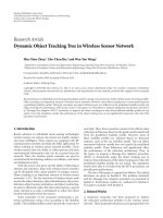
Figure 1: Audio key-finding system (fundamental + extensions).
simply reported one overall statistic for key-finding perfor-
mance [3, 7–9], which fails to fully address the importance
of the various components in the system, or the actual musi-
cal content, to system performance. We represent a solution
to audio key finding as a system consisting of several alter-
native parts in v arious stages. By careful analysis of system
performance with respect to choice of components in each
stage, we attempt to give a clearer picture of the importance
of each component, as well as the choice of music data for
testing, to key finding. Our approach draws inspiration from
multiple domains: from music theory to audio signal pro-

cessing. The system components we introduce aim to solve
the problem from different viewpoints. The modular design
allows us explore the strengths and weaknesses of each alter-
native option, so that the change in system performance due
to each choice can be made clear.
The rest of the paper is organized as follows. Section 1.1
provides a literature review of related work in audio key find-
ing. Section 2 describes the overall system diagram, with new
alternatives and extensions. The basic system, the FACEG
system, and the three key determination policies, the nearest-
neighbor (NN), relative distance (RD), and average distance
(AD) policies, are introduced in Section 3. The evaluation of
the FACEG system with the three key determination policies
follows in Section 4. Two case studies based on the musical
score are examined to illustrate situations in which audio key
finding performs better than symbolic key finding. Section 5
describes three extensions of the system: the modified spi-
ral array (mSA) approach, fundamental frequency identifica-
tion (F0), and post-weight balancing (PWB). Qualitative and
quantitative analyses and evaluations of the three extensions
are presented in Section 6. Section 7 concludes the paper.
1.1. Related work
Various state-of-the-art Audio key-finding systems were pre-
sented in the audio key-finding contest for MIREX [10].
Six groups participated in the contest, including Chuan and
Chew [11], G
´
omez [12],
˙
Izmirli [13], Pauws [14], Purwins

and Blankertz [15], and Zhu (listed alphabetically) [16].
Analysis of the six systems reveals that they share a similar
structure, consisting of some signal processing method, au-
dio characteristic analysis, key template construction, query
formation, key-finding method, and key determination cri-
teria. The major differences between the systems occur in
the audio characteristic analysis, key template construction,
and key determination criteria. In G
´
omez’s system, the key
templates are precomputed, and are generated from the
Krumhansl-Schmuckler pitch-class profiles [5], with alter-
ations to incorporate harmonics characteristic of audio sig-
nals. Two systems employing different key determination
strategies are submitted by G
´
omez: one using only the start
of a piece, and the other taking the entire piece into ac-
count. In
˙
Izmirli’s system, he constructs key templates from
monophonic instruments samples, weighted by a combina-
tion of the K-S and Temperley’s modified pitch-class profiles.
˙
Izmirli’s system tracks the confidence value for each key an-
swer, and the global key is then selected as the one having the
highest sum of confidence values over the length of the piece.
The key templates in Pauws’ and Purwins-Blankertz systems
are completely data-driven. The parameters are learned from
training data. In their systems, the key is determined based

on some statistical measure, or maximum correlation. In
contrast, Zhu builds a rule-based key-finding system; the
rules are learned from the MIDI training data. Further de-
tails of our comparative analysis of the systems can be found
in [11].
2. SYSTEM DESCRIPTION
Consider a typical audio key-finding system as shown schem-
atically in the top part of Figure 1. The audio key-finding sys-
tem consists of four main stages: processing of the audio sig-
nal to determine the frequencies present, determination of
the pitch-class description, application of a key-finding algo-
rithm, and key answer determination. Results from the key-
finding algorithm can give feedback to the pitch-class genera-
tion stage to help to constrain the pitch-class description to a
reasonable set. In this paper, we will consider several possible
alternative methods at each stage.
For example, as the basis for comparison, we construct a
basic system that first processes the audio signal using the fast
Fourier transform (FFT) on the all-frequency signal, then
generates pitch-class information using a fuzzy analysis (FA)
technique, calculates key results using the CEG algorithm
with a periodic cleanup procedure, and applies key determi-
nation policy to output the final answer. This basic system,
shown in the gray area in Figure 1, is described in detail in
C H. Chuan and E. Chew 3
Section 3, followed by an evaluation of the system using 410
classical pieces in Section 4.InSection 5, we present the de-
tails of several alternative options for the different stages of
the audio key-finding system. In the audio processing stage,
the two alternatives we consider are performing the FFT on

the all-frequency signal, or separating the signal into low
and high frequencies for individual processing. In the pitch-
class generation stage, the options are to use the peak detec-
tion method with fuzzy analysis, to use peak detection with
fundamental frequency identification, or to determine pitch
classes using sound sample templates. In the key determi-
nation stage, we consider the direct application of the spi-
ral array CEG Algorithm [1, 2], the CEG method with feed-
back to reduce noise in the pitch-class information, and the
CEG method with post-weight balancing. The lower part of
Figure 1 shows the various combinations possible, with the
alternate modules proposed, in assembling a key-finding sys-
tem. The in-depth evaluation and qualitative analysis of all
approaches are given in Section 6.
3. BASIC SYSTEM
We first construct our basic audio key-finding system as the
main reference for comparison. This system, shown in the
shaded portions of Figure 1, consists of first an FFT on the
audio sample. Then, we use the peak detection method de-
scribed in Section 3.1 and fuzzy analysis technique proposed
in Section 3.2 to generate a pitch-class description of the au-
dio signal. Finally, we map the pitch classes to the spiral array
model [1] and apply the CEG algorithm [2] to determine the
key. Distinct from our earlier approach, we explore here three
key determination policies: nearest-neighbor (NN), relative
distance (RD), and average distance (AD). Each method is
described in the subsections below. We provide an evaluation
of the system in Section 4.
3.1. Peak detection
We use the standard short-term FFT to extract frequency in-

formation for pitch identification. Music consists of streams
of notes; each note has the properties pitch and duration.
Pitch refers to the perceived fundamental frequency of the
note. The peak values on the frequency spectrum correspond
to the fundamental frequencies of the pitches present, and
their harmonics. We use the frequency at the peak value to
identify the pitch height, and map the peak spectral magni-
tude to the pitch weight. Pitches are defined on the logarith-
mic scale in frequency. A range of frequencies, bounded by
the midpoints between the reference frequencies, is deemed
acceptable for the recognition of each pitch. We focus our at-
tention on the pitches in the range between C
1
(32 Hz) and
B
6
(1975 Hz), which covers most of the common pitches in
our music corpus.
We synthesize audio wave files from MIDI at 44.1kHz
and with 16-bit precision. We process audio signal using FFT
with nonoverlapped Hanning windows. The window size is
setat0.37 second, corresponding to N
= 2
14
samples. Other
sample sizes were tested in the range of 2
10
to 2
15
(i.e., win-

dow size of 0.0232 to 0.74 second), but these did not perform
as well. Let x(n) be the input signal, where n
= 0, , N − 1.
The power spectrum is obtained using the equation
X(k)
=
1
N
N−1

n=0
x( n)W
kn
N
,(1)
where W
N
= e
− j2π/n
,andk = 0, 1, , N − 1. We then calcu-
late the magnitude from the power spectr um as follows:
M(k)
=


X(k)


=



X(k)
2
real
+ X(k)
2
img

. (2)
We set the reference fundamental frequency of A
4
at 440 Hz.
Let h(p) be the number of half steps between a pitch p and
the pitch A
4
.Forexample,h(p) =−9 when p = C
4
.The
reference fundamental frequency of pitch p is then given by
F0
ref
(p) = 440 × 2
h(p)/12
. (3)
We employ a local maximum selection (LMS) method [7]to
determine the presence of pitches and their relative weights.
The midpoint between two adjacent reference fundamen-
tal frequencies forms a boundary. We examine M(k) in the
frequency band between two such adjacent boundaries sur-
rounding each pitch p. The LMS method is based on two

assumptions: (1) a peak value should be larger than the av-
erage to its left and to its right in the given frequency band;
and (2) only one (the largest) peak value should be chosen
in each frequency band. The value M(k) satisfying the above
conditions for the frequency band around p, M
∗
(p), is cho-
sen as the weight of that pitch. This method allows us to con-
sider each pitch equally, so that the system is unaffected by
the logarithmic scale of pitch frequencies.
We apply the FFT to the audio signals w ith two differ-
ent setups. Under the first option, we process the signal as
a whole, with a window size of 0.37 second, to generate the
frequency magnitude for each pitch. In the second option,
we partition the signals into two subbands, one for higher
pitches (frequencies higher than 261 Hz, i.e., pitches higher
than C
4
), and one for lower ones. We use the same window
size to process the higher-pitch signals, and use a larger and
overlapped w indow size for the lower-pitch signals. The win-
dow size is relatively large compared to the ones typically
used in transcription systems. We give two main reasons for
our choice of window size. First, a larger window captures the
lower pitches more accurately, which provide the more valu-
able pitch information in key finding. Second, a larger win-
dow smoothes the pitch information, allowing the method
to be more robust to pitch variations less important to key
identification such as grace notes, passing tones, non-chord
tones, and chromatic embellishments.

3.2. Fuzzy analysis technique
The peak detection method described above generates pitch-
class distributions with limited accuracy. We design the fuzzy
analysis technique to clarify the frequency magnitudes ob-
tained from the FFT, in order to generate more accurate
pitch-class distributions for key finding. The main idea be-
hind the fuzzy analysis technique is that one can verify the
4 EURASIP Journal on Advances in Signal Processing
existence of a pitch using its overtone series. Hence, we can
emphasize the weight of a pitch that has been validated by
its overtone series, and reduce the weight of a pitch that has
been excluded due to the absence of its strongest overtones.
The problems stem from the fact that mapping of the
frequency magnitude directly to pitch weight as input to a
key-finding algorithm results in unbalanced pitch-class dis-
tributions that are not immediately consistent with existing
key templates. We have identified several sources of errors
(see [3]) that include uneven loudness of pitches in an audio
sample, insufficient resolution of lower-frequency pitches,
tuning problems, and harmonic effects. In spite of the un-
balanced pitch-class distributions, the key answer generally
stays within the ballpark of the correct one, that is, the an-
swer given is t ypically a closely related key. Some examples of
closely related keys are the dominant major/minor, the rela-
tive minor/major, and the parallel major/minor keys.
The fuzzy analysis technique consists of three steps. The
first step uses information on the overtone series to clarify the
existence of the pitches in the lower frequencies. The second
step, which we term adaptive level weighting, scales (multi-
plies) the frequency magnitudes by the relative signal density

in a predefined range, so as to focus on frequency ranges con-
taining most information. After the frequency magnitudes
have been folded into twelve pitch classes, we apply the third
step to refine the pitch-class distribution. The third step sets
all normalized pitch class values 0.2 and below to zero, and
all values 0.8 and above to one. Details of each step are given
below. After the three-part fuzzy analysis technique, we in-
troduce the periodic cleanup procedure for preventing the
accumulation of low-level noise over time.
Clarifying lower frequencies
In the first step, we use the overtone series to confirm the
presence of pitches below 261 Hz (C
4
). Because of the log-
arithmic scale of pitch frequencies, lower pitches are more
closely located on the linear frequency scale than higher ones.
The mapping of lower frequencies to their corresponding
pitch number is noisy and error prone, especially when us-
ing discrete frequency boundaries. There exists greater sep-
aration between the reference frequencies of higher pitches,
and the mapping of higher frequencies to their correspond-
ing pitches is a more accurate process. For lower pitches, we
use the first overtone to confirm their presence and refine
their weights.
We use the idea of the membership value in fuzzy logic
to represent the likelihood that a pitch has been sounded.
Assume that P
i, j
represents the pitch of class j at register
i, for example, middle C (i.e., C

4
)isP
4,0
. We consider the
pitch range i
= 2,3, 4, 5, 6, and j = 1, , 12, which includes
pitches ranging from C
2
(65 Hz) to B
6
(2000 Hz). The mem-
bership value of P
i, j
is defined as
mem

P
i, j

=
M
∗

P
i, j

max
p

M

∗
(p)

. (4)
Next, we define the membership negation value for lower
pitches, a quantity that represents the fuzzy likelihood that
a pitch is not sounded. Let the membership negation value
be
∼ mem

P
i, j

=
max

mem

P
i, j+1

,mem

P
i+1, j

,mem

P
i+1, j+1


,
(5)
where i
= 2, 3 and j = 1, ,12,becauseweconsideronly
the lower-frequency pitches, pitches below C
4
.Thisvalueis
the maximum of the membership values of the pitch one
half-step above (P
i, j+1
), and the first overtones of the pitch
itself (P
i+1, j
), and that of the pitch one half-step above the
first overtone. The membership value of a l ower-frequency
pitch is set to zero if its membership negation value is larger
than its membership value:
mem

Pi
j

=
⎧
⎨
⎩
0if∼ mem

P

i, j

> mem

Pi
j

,
mem

Pi
j

if ∼ mem

Pi
j

≤
mem

Pi
j

,
(6)
where i
= 2, 3 and j = 1, , 12. This step is based on the idea
that if the existence of the pitch a half-step above, as indicated
by mem(P

i, j+1
) and mem(P
i+1, j+1
), is stronger than that of
the pitch itself, then the pitch itself is unlikely to have been
sounded. And if the signal for the existence of the pitch is
stronger in the upper registers, then we can ignore the mem-
bership value of the present pitch.
Adaptive level weighting
The adaptive level weight for a given range, a scaling factor,
is the relative density of signal in that range. We scale the
weight of each pitch class by this adaptive level weight in or-
der to focus on the regions with the greatest amount of pitch
information. For example, the adaptive level weight for reg-
ister i (which includes pitches C
i
through B
i
), Lw
i
,isdefined
as
Lw
i
=

12
j=1
M


P
i, j


6
k
=2

12
j
=1
M

P
k, j

,(7)
where i
= 2, , 6. We generate the weight for each pitch
class, mem
C
(C
j
), by summing the membership values of that
pitch over all registers, and multiplying the result by the cor-
responding adaptive level weight:
mem
C

C

j

=
6

i=2
Lw
∗
i
mem

P
i, j

,(8)
where j
= 1, , 12.
Flatten high and low values
To reduce minor differences in the membership values of im-
portant pitch classes, and to eliminate low-level noise, we in-
troduce the last step in this section. We set the pitch-class
membership values to one if they are greater than 0.8, and
zero if they are less than 0.2 (constants determined from
held-out data). This flat output for high membership values
prevents louder pitches from dominating the weight.
C H. Chuan and E. Chew 5
Periodic cleanup procedure
Based on our observations, errors tend to accumulate over
time. To counter this effect, we implemented a periodic
cleanup procedure that takes place every 2.5 seconds. In this

cleanup step, we sort the pitch classes in ascending order and
isolate the four pitches with the smallest membership values.
We set the two smallest values to zero, a reasonable choice
since most scales consist of only seven pitch classes. For the
pitch classes with the third and fourth smallest membership
values, we consult the current key assigned by the CEG algo-
rithm; if the pitch class does not belong to the key, we set the
membership value to zero as well.
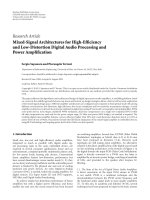
3.3. Spiral array model and the center of
effect algorithm
The spiral arr ay model, proposed by Chew in [1], is a
three-dimensional model that represents pitches, and any
pitch-based objects that can be described by a collection of
pitches, such as intervals, chords, and keys, in the same three-
dimensional space for easy comparison. On the spiral array,
pitches are represented as points on a helix, and adjacent
pitches are related by intervals of perfect fifths, while verti-
cal neighbors are related by major thirds. The pitch spiral is
shown on Figure 2(a). Central to the spiral array is the idea
of the center of effect (CE), the representing of pitch-based
objects as the weighted sum of their lower-level components.
The CE of a key is shown on Figure 2(b). Further details for
the construction of the spiral array model are given in [1, 2].
In the CEG algorithm, key selection is performed by a
nearest-neighbor search in the spiral array space. We will call
this the nearest-neighbor (NN) policy for key determination.
The pitch classes in a given segment of music is mapped to
their corresponding positions in the spiral array, and their CE
generated by a linear weighting of these pitch positions. The
algorithm identifies the most likely key by searching for the

key representation closest to the CE. The evolving CE creates
a path that tr aces its dynamically changing relationships to
the chord and key structures represented in the model [17].
Previous applications of the CEG algorithm have used the
relative pitch durations as the CE weights, either directly [2]
or through a linear filter [ 17]. Here, in audio key finding, we
use the normalized pitch-class distribution derived from the
frequency weights to generate the CE.
One more step remains to map any numeric representa-
tion of pitch to its letter name for key analysis using the spiral
array. The pitch spelling algorithm, described in [18, 19], is
applied to assign letter names to the pitches so that they can
be mapped to their corresponding representations in the spi-
ral array for key finding. The pitch spelling algorithm uses
the current CE, generated by the past five seconds of mu-
sic, as a proxy for the key context, and assigns pitch names
through a nearest-neighbor search for the closest pitch-class
representation. To initialize the process, all pitches in the first
time chunk are spelt closest to the pitch class D in the spiral
array, then the CE of these pitches is generated, and they are
respelt using this CE.
Major 3rd
Perfect 5th
(a)
CE of key
Tonic
(b)
Figure 2: (a) Pitch spiral in the spiral array model, and (b) the gen-
erating of a CE to represent the key.
If |d

j,t
− d
k,t
| <d,
If
d
i,t
< d
k,t
,
choose key i as the answer;
Else, choose key k as the answer;
Else, choose key i as the answer.
Algorithm 1: Related distance policy.
3.4. Key determination: relative distance policy
In the audio key-finding systems under consideration, we
generate an answer for the key using the cumulative pitch-
class information (from time 0 until the present) at every
analysis window, which eventually evolves into an answer for
the global key for the whole duration of the music example.
Directly reporting the key with the shor test distance to CE a s
the answer at each analysis window, that is, the NN policy,
does not fully reflect the extent of the tonal analysis infor-
mation provided by the spiral array model. For example, at
certain times, the CE can be practically equidistant from two
different keys, showing strong ambiguity in key determina-
tion. S ometimes the first key answer (the one with the short-
est distance to CE) may result from a local chord change, ca-
dence, or tonicization, and the second answer is actually the
correct global key. The next two key determination policies

seek to address this problem.
We first introduce the relative distance key determination
policy with distance threshold d, notated (RD, d). In the RD
policy, we examine the first two keys with the shortest dis-
tances to the CE. If the distance difference between the first
two keys is larger then the threshold d, we report the first
key as the answer. Otherwise, we compare the average dis-
tances of the two keys from the beginning to the current time
chunk. The one with shorter average distance is reported as
the answer.
Formally , let d
i, j
be the distance from the CE to key i at
time j,wherei
= 1, , 24. At time t, assume that keys i and
k are the closest keys to the CE with distances d
j,t
and d
k,t
,re-
spectively. Algorithm 1 describes the (RD,d) policy in pseu-
docode.
TheRDpolicyattemptstocorrectfortonalambiguities
introduced by local changes. The basic assumption underly-
ing this method is that the NN policy is generally correct.
6 EURASIP Journal on Advances in Signal Processing
In cases of ambiguity, which are identified as moments in
time when the first and second closest keys are less than the
threshold distance apart from each other, then we use the
average distance policy to determine which among the two

most likely candidates is the best choice. The next section de-
scribes the average distance policy in greater detail.
In this paper, we test two values of d. The choice of d
depends on the distance between keys in the spiral array. As-
sume d
1
denotes the shortest, and d
2
the second shortest, dis-
tance between any two keys in the spiral array model. Then
we constrain the value of d to the range
αd
1
≤ d ≤ βd
2
,(9)
where 0 <α, β
≤ 0.5. In this paper we set both α and β
equal to 0.25. Intuitively, this means that the CE should lie in
the center half of the line segment connecting two very close
keys, if there is ambiguity between the two keys.
3.5. Key determination: average distance policy
The average distance key determination policy (AD) is in-
spired by the method used by
˙
Izmirli in his winning sub-
mission to the MIREX 2005 audio key-finding competition
[13, 20], where only the global key answer w as evaluated.
˙
Izmirli’s system tracks the confidence value for each key an-

swer, a number based on the correlation coefficient between
the query and key template. The global key was then selected
as the one having the highest sum of confidence values over
the length of the piece.
In the spiral array, the distance from each key to the cur-
rent CE can serve as a confidence indicator for that key. In
the AD policy, we use the average distance of the key to the
CE at all time chunks to choose one key as the answer for the
whole testing duration of the piece.
Formally , at time t,if
d
j,t
= MIN
i=1, ,24

d
i,t

,choosekeyj as the answer. (10)
We explore the advantages and the disadvantages of the (RD,
d) and (AD) policies in the rest of the paper.
4. EVALUATION OF THE BASIC SYSTEM
In this paper we test the systems in two stages. In the first
stage, we use 410 classical music pieces to test the basic sys-
tems described in Section 3, that is, the audio key-finding
system using fuzzy analysis and the CEG algorithm, with the
three key determination policies, (NN), (RD, d), and (AD).
Both the local key answer (the result at each unit time) and
the global key answer (one answer for each sample piece) are
considered for the ev aluation. The results are analyzed and

classified by key relationships, as well as stylistic periods. At
the second stage of the evaluation, we use audio recordings of
24 Chopin Preludes to test the extensions of the audio key-
finding system.
We choose excerpts from 410 classical music pieces by
various composers across different time and stylistic peri-
ods, ranging from Baroque to Contemporary, to evaluate the
Table 1: Results analysis of global key answers across periods ob-
tained from fuzzy analysis technique and CEG algorithm.
Categories Baro
∗
Class
Early
Roman
Late
Con.
roman. roman.
CORR ∗∗ 80 95.772.47672.982.8
DOM 16.80 25.38 5.90
SUBD 0 0.90 4 0 1
REL 0 0.90 6 5 3
PAR 2.11.70 2 1 1
Others 0 0.92.34 10
Num. 95 115 87 50 34 29
∗
Baro = baroque, Class = classical, Roman = romantic, Con. =
contemporary.
∗∗
CORR = correct, DOM = dominant, SUBD = subdominant,
REL

= relative, PAR = parallel, Other = other.
methods. Table 1 shows the distribution of pieces across the
various classical genres. Most of the chosen pieces are concer-
tos, preludes, and symphonies, which consist of polyphonic
sounds from a variety of instruments. We regard the key of
each piece stated explicitly by the composer in the title as the
ground truth for the evaluation. We use only the first fifteen
seconds of the first movement so that the test samples are
highly likely to remain in the stated key for the entire dura-
tion of the sample.
In order to facilitate comparison of audio key finding
from symbolic and audio data, we collected MIDI sam-
ples from , and used the
Winamp software with 44.1 kHz sampling rate to render
MIDI files into audio (wave format). We concurrently tested
four different systems on the same pieces. The first system
applied the CEG algorithm with the nearest-neighbor pol-
icy, CEG(NN) to MIDI files, the second applied the CEG
algorithm with the nearest-neighbor policy and fuzzy anal-
ysis technique, FACEG(NN), and the third and the fourth
are similar to the second with the exception that they
employ the relative distance policy in key determination,
FACEG(RD, d), with different distance thresholds. The last
system, FACEG(AD), applies the relative distance policy with
average distances instead.
Two types of results are shown in the following sections.
Section 5.1 presents the averages of the results of all periods
over time for the four systems. Each system reported a key
answer every 0.37 second, and the answers are classified into
five categories: correct, dominant, relative, parallel, and oth-

ers. Two score-based analyses are given to demonstrate the
examples in which audio key-finding system outp erforms the
MIDI key-finding system that takes explicit note information
as input. In Section 5.2, the global key results given by the
audio key-finding system with fuzzy analysis technique and
CEG algorithm are shown for each stylistic period.
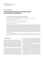
4.1. Overall results over time
Figure 3(a) shows the average correct rates of the five systems
over time on 410 classical music pieces. We can observe that
C H. Chuan and E. Chew 7
in the second half of the testing period, from 8 to 15 seconds,
four of the systems, all except FACEG(AD), achieve almost
the same results by the percentage correct measure.
The relative distance key determination policy using av-
erage distance FACEG(AD) performed best. Its correct per-
centage is almost 10% higher than the other systems from
8 to 15 seconds. Notice that the improved correct rate of
FACEG(AD) is mainly due to the reduction of dominant and
relative errors shown in Figures 3(b) and 3(c). The relative
distance policy using threshold distance (RD, d) slightly out-
performs the systems with only the nearest-neighbor (NN)
policy in audio key finding. The results of the systems with
the RD and AD policies maintain the same correct rates from
5 seconds to the end. The longer-term stability of the results
points to the advantage of the RD and AD policies for choos-
ing the global key.
The CEG(NN) system outperforms all four audio sys-
tems in the first five seconds. The RD policy even lowers
the correct rate of the FACEG(NN) audio key-finding sys-
tem. The results show that audio key-finding system requires

more time at the beginning to develop a clearer pitch-class
distribution. The RD policy may change correct answers to
the incorrect ones at the beginning if the pitch-class infor-
mation at the first few seconds is ambiguous.
Figures 3(b) to 3(e) illustrate the results in dominant,
relative, paral lel, and others categories. Most differences be-
tween the CEG(NN) system and the FACEG audio key-
finding systems can be explained in the dominant and paral-
lel errors, shown in Figures 3(b) and 3(d).Wecanusemusic-
theoretic counterpoint rules to explain the errors. In a com-
position, doubling of a root or the fifth of a chord is pre-
ferred over doubling the third. The third is the distinguishing
pitch between major and minor chords. When this chord is
the tonic, the reduced presence of thirds may cause a higher
incidence of parallel major/minor key errors in the first four
seconds. For audio examples, the third becomes even weaker
because the harmonics of the root and the fifth are more
closely aligned, which explains why audio key-finding sys-
tems have more parallel errors than the MIDI key-finding
system CEG(NN). The ambiguity between parallel major and
minor keys subsides once the system gathers more pitch-class
information.
In the relative and other error categories, shown in Fig-
ures 3(c) and 3(e), the audio key-finding systems perform
slightly better than the MIDI key-finding system. We present
two examples with score analysis in Figures 4 and 5 to
demonstrate how the audio key-finding systems—FACEG
(NN), FACEG (RD, 0.1), FACEG (RD, 0.17), FACEG (AD)—
outperform the MIDI key-finding system.
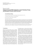
4.2. When audio outperforms symbolic key finding

Figure 4 shows the first four measures of Bach’s Double Con-
certo in D minor for two violins, BWV1043. For the whole
duration of the four measures, all audio systems give the cor-
rect key answer, D minor. In contrast, the MIDI key-finding
system returns the answer F major in the first two measures,
80
75
70
65
60
55
50
Correct rate (%)
0 1 2 3 4 5 6 7 8 9 10 11 12 13 14 15
Time (s)
(a) Correct rate (%)
18
16
14
12
10
8
6
4
2
Dominant error (%)
0 1 2 3 4 5 6 7 8 9 10 11 12 13 14 15
Time (s)
(b) Dominant error (%)
7

5
3
1
Relative error (%)
0 1 2 3 4 5 6 7 8 9 10 11 12 13 14 15
Time (s)
(c) Relative error (%)
18
16
14
12
10
8
6
4
2
0
Parallel error (%)
0 1 2 3 4 5 6 7 8 9 10 11 12 13 14 15
Time (s)
(d) Parallel error (%)
18
16
14
12
10
8
6
4
2

Other error (%)
0 1 2 3 4 5 6 7 8 9 10 11 12 13 14 15
Time (s)
CEG (NN)
FACEG (NN)
FACEG (RD, 0.1)
FACEG (RD, 0.17)
FACEG (AD)
(e) Other error (%)
Figure 3: Results of first fifteen seconds of 410 classical pieces, clas-
sified into five categories.
8 EURASIP Journal on Advances in Signal Processing
Pitch class distribution (MIDI)
0.2
0.1
0
CDEFGABb
Pitch class distribution (audio)
0.16
0.1
0
CDEF GABb
MIDI: F major, audio: D minor
Violin I
Violin II
Piano
MIDI: G major, audio: D minor
Pitch class distribution
(MIDI)
0.3

0.2
0.1
0
CDEFGABb
(audio)
Pitch class distribution
0.18
0.1
0
CDEF GABb
Figure 4: Pitch-class distribution of Bach concertos in D minor.
then changes the answer to G major at the end. We can ex-
plain the results by studying the pitch-class distributions for
both the MIDI and audio systems at the end of the second
and fourth measures.
The pitch-class distribution of the MIDI system at the
second measure does not provide sufficiently significant dif-
ferences between the pitch sets belonging to F major and D
minor; however, the high weight on pitch class A, the second
harmonic of the pitch D, in the corresponding distribution
derived from audio helps to break the tie to result in the an-
swer, D minor. At the end of the second measure and the
beginning of the third, there are two half-note G’s in the bass
line of the piano par t. These relatively long notes bias the an-
swer towards G major in the MIDI key-finding system. The
audio key-finding systems are not affected by these long notes
because the effect of the overlapping harmonics results in a
strong D, and a not-as-high weight on G in the pitch-class
distribution.
We give another example in Figure 5, which shows the

firsteightmeasuresofBrahms’Symphony No. 4 in E mi-
nor, Op.98. Both the MIDI and audio key-finding systems
report correct answers for the first six measures. At measures
6 through 8, the chords progress from vi (pitches C, E, G)
to III (pitches G, B, D) to VII (pitches D, F
#
, A) in E minor,
which correspond to the IV, I, and V chords in G major. Af-
ter these two measures the answer of the MIDI key-finding
system becomes G major. This example shows that having
explicit information of only the fundamental pitches present
makes the MIDI key-finding system more sensitive to the lo-
cal tonal changes.
4.3. Results of global key across periods
We use the average of the distances between the CE and
the key over all time chunks to determine the global key.
The one which has the shortest average distance is chosen
to be the answer. Tabl e 1 lists the results of global key an-
swers, broken down by stylistic periods, obtained from the
audio key-finding, FACEG(AD), systems. The period classi-
fications are as follows: Baroque (Bach and Vivaldi), Classical
(Haydn and Mozart), Early Romantic (Beethoven and Schu-
bert), Romantic (Chopin, Mendelssohn, and Schumann),
Late Romantic (Brahms and Tchaikovsky), and Contempo-
rary (Copland, Gershwin, and S hostakovich). The results
themselves are separated into six categories as well: Cor rect,
Dominant, Subdominant, Relative, Parallel, and Other (in
percentages).
Notice that in Tab le 1 , the results vary significantly from
one period to another. The best results are those of the Clas-

sical period, which attains the highest correct percentage
rate of 95.7% on 115 pieces. The worst results are those of
pieces from the Early Romantic period, having many more
C H. Chuan and E. Chew 9
Pitch class distribution (MIDI)
0.3
0.2
0.1
0
CDEF GAB
Pitch class distribution (audio)
0.2
0.1
0
CDEF
#
GAB
MIDI: E minor, audio: E minor
2Flute
2 klarinette in A
2fagotte
In E
1
2
4horner
In C
2
4
1. violine
2. violine

Bratsche
Violoncell
Kontraba 3
MIDI: G major, audio: E minor
Allegro non troppo
Pitch class distribution (MIDI)
0.3
0.2
0.1
0
CDEF
#
GAB
distribution
(audio)
Pitch class
0.2
0.1
0
CDEF
#
GAB
Figure 5: Pitch-class distributions of Brahms symphony number 4 in E minor.
errors on the dominant and others categories. The variances
in Tab le 1 show clearly the dependency between the system
performance and the music style. Lower correct rates could
be interpreted as an index of the difficulty of the test data.
5. SYSTEM EXTENSIONS
In this section, we propose three new alternatives for the
pitch-class generation and the key-finding stages to improve

audio key finding as was first presented in the system out-
line given in Figure 1. These methods include modifying the
spiral array model using sampled piano audio signals, funda-
mental frequency identification, and post-weight balancing.
The three approaches affect different stages in the prototyp-
ical system, and use different domains of knowledge. In the
first alternative, we modify the spiral ar ray model so that the
positions of the tonal entities reflect the frequency features of
audio signals. The second alternative affects pitch-class gen-
eration; we use the information from the harmonic series to
identify the fundamental frequencies. The third method of
post-weight balancing is applied after the key-finding algo-
rithm; it uses the key-finding answer to refine the pitch-class
distribution. Each of the three approaches is described in the
subsections to follow.
5.1. Modified spiral array with piano signals
Since the pitch-class distribution for each audio sample is
constructed using the frequency magnitudes derived from
the FFT, in order to compare the CE of this distribution to
an object of the same type, we propose to prepare the spiral
array to also generate tonal representations based on audio-
signal frequency features. In this section, we describe how
we modify the major and minor key spirals so that the po-
sitions of key spirals are constructed according to the fre-
quency features of the audio signals. The advantages of the
proposed modification are that the modified spiral array can
manage the diversity of the frequency features of audio sig-
nals, and tolerate the errors from pitch detection method. A
similar idea is proposed by
˙

Izmirli to modify the Krumhansl-
Schmuckler key-finding method to address audio signals in
[13].
Figure 6 shows the sequence of steps for remapping the
spiral array representations for audio. The mapping uses the
10 EURASIP Journal on Advances in Signal Processing
Monophonic
pitch sample
Peak detection
fuzzy analysis
Classifier
Calculate
pitch
position
Calculate
pitch
position
Figure 6: System diagram of reconstructing pitches in spiral array
model.
frequency distribution of monophonic pitch samples to first
classify pitches into subclasses based on their harmonic pro-
file, then calculates the new position of each pitch for each
subclass. The monophonic pitch samples, piano sounds from
Bb
0
to C
8
, are obtained from the University of Iowa Musi-
cal Instrument Samples online [21]. The classification step
is essential because tone samples from different registers ex-

hibit different harmonic characteristics. Hence, the represen-
tations are regenerated for each subclass.
Formally, for each monophonic pitch sample, we apply
the peak detection method and fuzzy analysis technique to
generate a pitch-class distribution for that pitch, mem(C
j
),
i
= 1,2, , 12. Each pitch then is classified into several sub-
classes according to the pitch-class distribution. The classifi-
cation can be done by any existing classifiers, such as k near-
est neighbors. The classification must satisfy the constraint
that each class consists of pitches that are close to one an-
other. This constraint is based on the assumption that pitches
in the same range are likely to have similar pitch-class distri-
butions. For the purposes of the tests in this paper, we classify
the pitches into five classes manually.
The new position of the pitch representation in the spiral
array, for each subclass, is recomputed using these weights.
Assume P
i
represents the original position of pitch class i in
the spiral array model. The new position of pitch class i, P

i
,
is defined as
Pi

=

1
n
12

j=1
mem

C
j

×
p
j
, (11)
where j
= 1, ,12andn is the size of the subclass. Figure 7
shows conceptually the generating of the new position for
pitch class C.
Once we obtain the new position of pitches, we can calcu-
late the new position of keys for each subclass by a weig h ted
linear combination of the positions of the triads. The com-
posite key spirals are generated in real time as the audio sam-
ple is being analyzed. We weight the key representation from
each subclass in a way similar to that for the level weights
method described in Section 3.2. That is to say, the level
weight for a given subclass is given by the relative density of
pitches from that subclass. The position of each key in a key
spiral is the sum of the corresponding key representations for
each subclass, multiplied by its respective level weight. As-
sume T

i
is the original position of key i in the spiral array,
the new position of key i, T

i
, is calculated by
T

i
= Lw
i
× T

j
, (12)
Revised CE
New pitch positions
Figure 7: Recalculating pitch position using pitch-class distribu-
tion.
0.5
0.4
0.3
0.2
0.1
0
0 100 200300400 500600700
Frequency (Hz)
(a)
1.4
1.2

0.8
0.4
0
0 100 200 300 400 500600700
Frequency (Hz)
(b)
Figure 8: Frequency responses of pitches (a) Bb
0
and (b) F
1
using
FFT.
where Lw
i
is the level weight for subclass i and T

j
is the com-
posite position for key j in subclass i, j
= 1, ,24 for 24
possible keys.
As the final step, we perform the usual nearest-neighbor
search between the CE generated by the pitch-class distribu-
tion of the audio sample and the key representations to de-
termine the key.
5.2. Fundamental frequency identification
Audio signals from music differ from speech signals in three
main aspects: the frequency range, the location of the funda-
mental frequency, and the characteristic of the harmonic se-
ries. Compared to human voices, instruments can sound in

a much wider range of frequencies. Furthermore, the lower
pitches are typically organized in such a way as to highline the
tonal structure of the music sample, while the higher pitches
are less important structurally, and may contain many su-
perfluous accidentals. However, the structur ally more im-
portant lower pitches cannot always be detected using sig-
nal processing methods such as the FFT. Also, se veral lower
pitches may generate similar distributions in the frequency
spectrum. Missing information in the lower registers seri-
ously compromises the results of key finding. Figure 8 shows
the FFT output for pitches Bb
0
and F
1
.Itisimportantto
note that these two pitches have similar frequency distribu-
tions, yet neither of their fundamental frequencies appear in
C H. Chuan and E. Chew 11
Table 2: Frequency and pitch relations of seven harmonics.
Frequency ratio 1 2 3 4 5 6 7
Pitch relation
∗∗∗
1 8va 8va + P5 16va 16va + M3 16va + P5 16va + m7
Semitone distance 0 12 19 24 28 31 34
∗∗∗
: P5: per fect fifth, M3: major third, m7: minor seventh.
the FFT. In the case of pitch Bb
0
, none of the pitches in the
pitch class Bb is presented. This example reveals a key consid-

eration as to why audio key finding frequently suffers from
dominant errors. The audio signals of each individual pitch
are collected from the piano recordings on the Iowa Univer-
sity website [21].
Many systems for automatic transcription that use fun-
damental frequency to identify pitch have been proposed re-
cently [22, 23]. The transcription problem requires the ex-
traction of multiple fundamental frequencies of simultane-
ously sounding pitches. We, instead, are concerned with find-
ing only the lowest pitch in the bass. We use the first seven
harmonics to identify each fundamental frequency. The fre-
quency ratio (multiple of the fundamental frequency) and
the pitch relation of the harmonic structure are given in
Table 2. We use this harmonic structure as a template for lo-
cating the fundamental frequencies as follows. Given an au-
dio signal, first we extract the frequencies with the largest and
second largest frequency magnitudes. Then we move the har-
monic template so as to find all possible ways to cover the
two frequencies, and calculate the total number of frequen-
cies that are both in the harmonic template and the extracted
frequency spectrum. The highest scoring option gives the lo-
cation of the fundamental frequency. We employ a heur istic
to break ties. Ties happen because not all the harmonics ap-
pear for a tone of a given fundamental pitch. When an octave
pair is encountered, it is unclear if this represents the funda-
mental pitch class, or the fifth above the fundamental. The
heuristic is based on our observations, and prefers the inter-
pretation of the fifth when finding an octave pair in the lower
registers.
Using a window size that is three times larger for low fre-

quencies than higher ones (0.37 second), we tested the above
method on monophonic piano samples of pitches ranging
from Bb
0
to B
3
obtained f rom the Iowa University website
[21]. For the 38 samples, we successfully identified the fun-
damental frequencies of 33 pitches, with 4 octave errors and
1 perfect fifth er ror. The octave error does not affect key find-
ing.
5.3. Post-weight balancing
In audio key finding, unbalanced pitch-class distribution is
often obtained using the frequency spectrum derived from
the FFT. One particularly problematic example occurs w hen
the weight of a certain pitch class is much higher than the
others. The pitch class dominates the weight distribution so
much so that the CE is strongly biased by that pitch class, and
cannot fairly represent the presence of the other pitch classes.
Let K
3
be the set of three closest keys and K
2
is any
subset with two keys of K
3
.
(1) If K
2
contains a relative major/minor pair, then the

tonic of K
3
\K
2
is labeled as overweighted.
(2) If K
2
contains a parallel major/minor pair, then the
tonic of K
2
is labeled as overweighted.
(3)Overweightedpitchclassisassignedtheaverage
weight of pitches in K
3
.
Algorithm 2: Post-weight balancing.
The relative distance policy in key determination, in which
the system compares the distance difference between the first
two keys, cannot solve this unbalanced distribution problem.
Similarly, one cannot readily eliminate the problem by sim-
ply examining the low-level features such as the frequency of
the audio signal.
To solve the problem of unbalanced weight distributions,
we design a post-weight balancing mechanism. We use high-
level knowledge of the relations between keys to determine
which pitch class has been weighted too heavily. The post-
weight balancing mechanism is based on two principles: (1)
if the three closest keys contain a relative major/minor pair,
then the tonic of the other key is likely overweighted; (2) if
the three closest keys contain a parallel major/minor pair,

then the tonic of the pair is likely overweighted.
Once the overweighted pitch class is identified, we re-
duce its weight in the pitch-class distribution, and reapply
the CEG algorithm to generate a new answer with the ad-
justed pitch-class distribution. The new answer is then ver-
ified again using the post-weig ht balancing mechanism to
specifically disambiguate the relative or parallel major/minor
answers. To differentiate between relative major/minor keys,
we compare the weights of the respective tonic pitch classes.
The one with larger weight is chosen as the answer. To dif-
ferentiate between parallel major/minor keys, we examine
the weights of the nondiatonic pitches in each candidate
key. The p ost-weight balancing algorithm is summarized in
Algorithm 2.
6. IN-DEPTH ANALYSIS OF RESULTS
In order to explore the possible approaches for improv-
ing audio key-finding system outlined in Section 5,wetest
five systems on Evgeny Kissin’s CD recordings of Chopin’s
Twenty-Four Preludes for piano (ASIN: B00002DE5F). We
chose this test set for three reasons: (1) it represents one of
12 EURASIP Journal on Advances in Signal Processing
80
70
60
50
40
30
20
10
Correct rate (%)

0123456789101112131415
Time (s)
Sys (FA, SA/CEG)
Sys (FA, SA/CEG, PWB)
Sys (mSA/CEG)
Sys (FA, mSA/CEG)
Sys (F0, SA/CEG)
Figure 9: Correct rate of five extended systems on Chopin’s 24 Pre-
ludes.
the most challenging key-finding datasets we have tested to
date—in a previous study (see [3]), we discovered that the
results for this test set was farthest from that for MIDI; (2) the
audio recording created using an acoustic piano allows us to
test the systems’ robustness in the presence of some timbral
effects; and (3) a minor but aesthetic point, all 24 keys are
represented in the collection.
The five systems selected for testing consist of combina-
tions of the approaches described in Sections 3 and 5,witha
focus on the three new alternatives introduced in Section 5.
We introduce a notation for representing the systems. The
fivesystemsareasfollows:
(a) the basic system, sys(FA, SA/CEG);
(b) FACEG with post-weight balancing, sys(FA, SA/CEG,
PWB);
(c) the modified spiral array with CEG, sys(mSA/CEG);
(d) FACEG with modified spiral array, sys(FA, mSA/CEG);
(e) fundamental frequency identification with CEG,
sys(F0, SA/CEG).
We have ascertained in Section 4.1 that the best key determi-
nation policy was the AD, average distance policy, which is

nowemployedinallfivesystems.
The first system, sys(FA, SA/CEG), serves as a reference,
a basis for comparison. The second system, sys(FA, SA/CEG,
PWB), tests the effectiveness of the post-weight balancing
scheme applied to the basic system. The fourth system,
sys(FA, mSA/CEG), tests the effectiveness of the modifica-
tions to the spiral array based on audio samples, in compari-
son to the basic system. To further test the power of the mod-
ified spiral array, we take away the fuzzy analysis layer from
(d) to arrive at the third system, sys(mSA/CEG). The fifth
system, sys(F0, SA/CEG), tests the effectiveness of the funda-
mental frequency identification scheme relative to the basic
system.
The overall results for all five extended s ystems are shown
in Figure 9. The system employing fundamental frequency
identification with the CEG algorithm, sys(F0, CEG), out-
performs the others in the first 8 seconds. The systems us-
ing the modified spiral array model, sys(mSA/CEG) and
SR R DR
STD
SP P DP
(a) Key map
022
0126
011
(b) FA, SA/CEG
014
1132
020
(c) FA, SA/CEG,

PWB
121
0163
000
(d) mSA/CEG
121
0173
000
(e) FA, mSA/CEG
131
0134
000
(f) F0, SA/CEG
Figure 10: Results of five systems on Chopin’s 24 Preludes T: tonic,
D: dominant, S: subdominant, R: relative, P: parallel.
Table 3: Summary of the results of five systems categorizing the
pieces by the number of the correct answers.
no. of sys w. corr. ans. 5 4 3 2 1 0
Piece 6, 8, 17, 14, 15, 2, 4, 10, 1, 3, 5, 9,
Prelude no. 19, 20, 24 21, 23 7, 12 22 11, 16 13, 18
sys(FA, mSA/CEG), achieve the best correct rates after 8 sec-
onds, and significantly higher correct rates from 12 to 15
seconds. In comparison to the original system, sys(FA, CEG),
the post-weight balancing used in sys(FA, CEG, PWB) im-
proves the results slightly.
Figure 10 shows the cross-section of results at fifteen sec-
onds for the five systems. Each result is represented in a key
map, where the tonic (the ground truth) is in the center, and
the dominant, subdominant, relative, parallel are to the right
and left, and above, and below the tonic, respectively. The

number inside each grid is the number of the answers that
fall in that category. Answers that are out of the range of the
key map are not shown.
Figure 10(b) shows the results of the original system, the
fuzzy analysis technique with spiral array CEG algorithm.
The results of system extensions are given in Figures 10(c)
through 10(f). Notice that the FACEG system with modi-
fied spiral array model, Figure 10(e), gets the most correct
answers, which implies that including the frequency features
within the model could be the most effective way to improve
the system. This result is confirmed by Figure 9.
In Tab le 3 , we categorize the pieces by the number of sys-
tems that report correct answers. By analyzing pieces with
the most or least number of correct answers, we can better
understand which kinds of musical patterns pose the great-
est difficulty for all systems, as well as the advantages of one
system over the others for certain pieces. The results summa-
rized in Tabl e 3 suggest that the ease of arriving at a correct
key solution is independent of the tempo of the piece.
C H. Chuan and E. Chew 13
0.9
0.7
0.5
0.3
0.1
Distance in spiral array
0 1 2 3 4 5 6 7 8 9 10 11
12
13 14 15
Time (s)

Eb major
C minor
G
A
Db
C minor
G
Db
Eb
Db
G
Db
Eb
g
D
C
minor
1st answer
2nd answer
Largo.
ff
Figure 11: Key answers over time of sys(FA, CEG) on Chopin’s Pre-
lude number 20 in C minor.
We now focus on the analysis of some best- and worst-
case answers for audio key finding. Chopin’s Prelude No. 20 in
Cminoris one of the pieces for which all of the systems gave
a correct answer, even though it could be interpreted as being
in four different keys in each of the first four bars. Figure 11
shows the first part of the score corresponding to the audio
sample analyzed, the audio wave of the first fifteen seconds,

and the top two key answers over time, and the distances of
these key representations to the CE of the audio sample. In
the spiral array model, shorter distances correspond to more
certain answers. The results over time presented in Figure 11
show the two key representations closest to the current cu-
mulative CE at each time sample. The closest answer is C
minor for most of the time, except from 8.14 to 13.32 sec-
onds, when the closest answer is Eb major, while C minor is
relegated to the second closest answer. The graph shows the
chord sequence’s brief tonicization in Eb major at the end of
measure three, before reaching G major at the end of mea-
sure four, which acts as the dominant to the key of C minor.
Chopin’s Prelude No. 9 in E major is an example in which
all five systems reported B major as the key, the dominant of
E. Figure 12 shows the score for the first part of the piece, the
audio wave of the first fifteen seconds, and the top two key
answers over time for the four audio systems. From Figures
12(a) to 12(d), we observe the following two common behav-
iors in all graphs: (1) for most of the time during the fifteen
seconds, the top-ranked answer is B major, while the second
answer traverses through related keys; and (2) the first and
second answers are almost equidistant from the CE in the
middle part, between 7 and 8 seconds.
The test duration (first fifteen seconds) corresponds to
the first two and half measures of the piece. From the score,
the chord progression of the first measure is I-V-I-IV in E
major, which unequivocally sets up the key as E major. The
dominant errors of all systems can be attributed to the au-
dio attributes of Evgeny Kissin’s expressive performance. In
the recording, Kissin emphasizes the pitch B

3
at each beat
C
G
E
f#
G
D
B
F#
F# b
b
b
bb
b
b
F#
F#
c
c
F# F#
c#
c#
Eb Eb
Eb
Eb
Eb
E
E
E

E
E
E
E
EE
b
Eb
Eb
D
D
c#
f#
G
Largo
f sostenuto
With Leo
0.35
0.25
0.15
0.05
Distance in spiral array
0 1 2 3 4 5 6 7 8 9 10 11 12 13 14 15
Time (s)
Bmajor
Bmajor
(a) sys(FA, SA/CEG)
C
C
G
E

f#
f#
G
G
D
B
F#
F#
b
b
b
b
b
b
b
F#
F#
F#
F#
F#
f#
f#
c#
c#
f#
f#
D
D
Eb
Eb

Eb
Eb
Eb
E
E
EE
E
E
E
E
Eb
0.35
0.25
0.15
0.05
Distance in spiral array
0 1 2 3 4 5 6 7 8 9 10 1112131415
Time (s)
Bmajor
Bmajor
(b) sys(FA, SA/CEG, PWB)
C
C
C
G
ea
D
B
b
b

b
b
e
e
e
B
E
E
G
c
g
a
a
e
G
b
A
B
e
B
b
A
A
F#
B
B
b
b
b
b

b
F#
F#
F#
g
g
g
b
b
F#
F#
F#
g
B
F#
F#
F#
F#
F#
0.35
0.25
0.15
0.05
Distance in spiral array
0 1 2 3 4 5 6 7 8 9 10 1112131415
Time (s)
Bmajor
Emajor
(c) sys(mSA/CEG)
C

C
C
G
e
D
G
B
B
b
b
b
b
e
e
e
e
B
B
B
c
c
g
e
E
G
C
b
b
A
B

e
B
b
b
b
F#
F#
B
bbb
b
f#
F#
F#
F#
F#
F#
F#
b
D
f# f#
b
b
b
bF
#
D
0.35
0.25
0.15
0.05

Distance in spiral array
0 1 2 3 4 5 6 7 8 9 10 11 12 13 14 15
Time (s)
Bmajor
Emajor
(d) sys(FA, mSA/CEG)
E
B
B
B
B
E
E
B
B
B
BB
B
B
e
e
b
b
b
F#
B
B
F#
F#
F#

D
D
F#
E
F#
0.35
0.25
0.15
0.05
Distance in spiral array
0 1 2 3 4 5 6 7 8 9 10 11 12 13 14 15
Time (s)
1st answer
2nd answer
(e) sys(F0, SA/CEG)
Figure 12: Key answers over time on Chopin’s Prelude number 9 in
Emajor.
14 EURASIP Journal on Advances in Signal Processing
as it is an important pitch that is repeated frequently in the
melodic line. The emphasis on the pitch B
3
, and later on the
lowest note B
1
, results in the larger weight of B in the pitch-
class distribution. Even though the notes in the score and the
chords as early as the first bar clearly show E major as the key,
the prominence of the pitch B in the performance overshad-
ows the answer so that B major and B minor appear most
frequently as top choices for this piece, even though the key

of E major is ranked first or second at least once in the first
two seconds for all systems.
The results in Figures 12(a) and 12(b) show that post-
weight balancing does not improve the answers in this case,
where the pitches emphasized in the expressive performance
dominate the results. The PWB method may be more ef-
fective if the parameters for the weight adjustments are op-
timized through learning. Compared with the other three
systems, the F0 method employed in system (e) appears to
have stabilized the results, and to react most sensitively to
changing pitches in the lower registers. Sys(F0, SA/CEG) gets
the correct answer within the first second, which is quicker
than the others. In (c) and (d), sys (mSA/CEG) and sys(FA,
mSA/CEG), the answers based on the modified spiral array
model, appear more random than the other systems, and
are difficult to explain directly from the score. Using the fre-
quency distribution of the pitches instead of the apparent du-
ration does not appear to have been very helpful in this case.
7. CONCLUSIONS AND DISCUSSION
We have presented a fundamental audio key-finding sys-
tem, FACEG, with three key determination policies of (NN),
(RD), and (AD). We evaluated the basic system by comparing
the results between the audio key-finding systems, with the
three different key determination policies, as well as a sym-
bolic key-finding system. We showed that the fundamental
audio key-finding system with the average distance key de-
termination policy, FACEG (AD), is superior as it achieves
generally 10% higher correct rates than the other systems. We
showed that the stylistic period of the classical pieces could be
used as an indicator for the difficulty of key finding for that

test set.
We also presented three possible extensions to the ba-
sic system: the modified spiral array (mSA), fundamen-
tal frequency identification (F0), and post-weight balancing
(PWB) scheme. We evaluated the three methods by con-
structing five audio key-finding systems with different com-
binations of possible extensions, and provided qualitative as
well as quantitative analyses of their key-finding performance
on recordings of Chopin’s Preludes for piano. We observed
that the fuzzy analysis system with the modified spiral array
performs best, by the average correct rate metric. The over-
all performance of the five systems matched our expectations
that identifying the fundamental frequencies is helpful in the
first 8 seconds when fewer notes have been sounded; and the
systems employing the modified spiral array, which incor-
porated audio frequency features in its weights, become the
most effective after 8 seconds, when more notes have been
played.
We further provided detailed analyses on the case when
all five audio systems gave the correct answer and on another
case when all five systems failed. The result of the case studies
presented some evidence against the summary statistics as a
metric for key finding, and demonstrated the specific advan-
tages and disadvantages of the system extensions.
Each of the improvements proposed to the specific sys-
tem addressed in this paper can also be employed in other
audio key-finding systems. For example, modifying an exist-
ing model with instr ument-specific signals (as in the mod-
ified spiral array method of Section 5.1) can be applied to
any other key matching algorithm, such as the Krumhansl-

Schmuckler method; fundamental frequency identification
(Section 5.2) can be applied to the transcription of mono-
phonic bass instruments, such as cello, with appropriate har-
monic templates; post-weight balancing (Section 5.3)canbe
directly plugged into any audio key-finding system for refin-
ing pitch-class distributions based on the key answer.
In this paper, our test data comprised of audio synthe-
sized from MIDI (mostly symphonies and concertos), and
of audio from acoustic piano. Methods such as the mod-
ified spiral array (Section 5.1), and post-weight balancing
(Section 5.3), and analyses of when audio outperforms MIDI
key finding (Section 4.2) can be highly dependent on the in-
strumental timbre of the training and test data. Timbre is a
variable that requires systematic study in the future.
The constant Q transform is another option for extract-
ing frequency information from audio signal. The constant
Q transform is closely related to the FFT, except that the
frequency-resolution ratio remains constant. This constant
ratio confers two major advantages to the constant Q: first,
with a proper choice of center frequency, the output of the
constant Q transform corresponds to musical notes; second,
the constant Q transform uses higher time resolutions for
higher frequencies, which better models the human auditory
system. One of the design choices for the present audio key-
finding system was to concentrate on lower frequencies, be-
causebassnotespresentstrongandstablecuesforthekey;
thus, our decision was to use the proposed fuzzy analysis
technique to confirm lower frequencies using the overtones.
In the future, we plan to explore other techniques using the
constant Q transform for audio key finding.

REFERENCES
[1] E. Chew, “Towards a mathematical model of tonality,” Doc-
toral dissertation, Department of Operations Research, Mas-
sachusetts Institute of Technology, Cambridge, Mass, USA,
2000.
[2] E. Chew, “Modeling tonality: applications to music cognition,”
in Proceedings of the 23rd Annual Meeting of the Cognitive Sci-
ence Society (CogSci ’01), pp. 206–211, Edinburgh, Scotland,
UK, August 2001.
[3] C H. Chuan and E. Chew, “Fuzzy analysis in pitch-class deter-
mination for polyphonic audio key finding,” in Proceedings of
the 6th International Conference on Music Information Retrieval
(ISMIR ’05), pp. 296–303, London, UK, September 2005.
[4] H. C. Longuet-Higgins and M. J. Steedman, “On interpreting
bach,” in Machine Intelligence, vol. 6, pp. 221–241, Edinburgh
University Press, Edinburgh, Scotland, UK, 1971.
C H. Chuan and E. Chew 15
[5] C. L. Krumhansl, “Quantifying tonal hierarchies and key dis-
tances,” in Cognitive Foundations of Musical Pitch,chapter2,
pp. 16–49, Oxford University Press, New York, NY, USA, 1990.
[6] D . Temperley , “What’s key for key? the Krumhansl-Schmu-
ckler key-finding algorithm reconsidered,” Music Perception,
vol. 17, no. 1, pp. 65–100, 1999.
[7] C H. Chuan and E. Chew, “Polyphonic audio key finding us-
ing the spiral array CEG algorithm,” in Proceedings of IEEE In-
ternational Conference on Multimedia and Expo (ICME ’05),
pp. 21–24, Amsterdam, The Netherlands, July 2005.
[8] E. G
´
omez and P. Herrera, “Estimating the tonality of poly-

phonic audio files: cognitive versus machine learning mod-
elling strategies,” in Proceedings of 5th International Confer-
ence on Music Information Retrieval (ISMIR ’04), pp. 92–95,
Barcelona, Spain, October 2004.
[9] S. Pauws, “Musical key extraction from audio,” in Proceedings
of 5th International Conference on Music Information Retrieval
(ISMIR ’04), pp. 96–99, Barcelona, Spain, October 2004.
[10] 1st Annual Music Information Retrieval Evaluation eX-
change, MIREX 2005, />Main
Page.
[11] C H. Chuan and E. Chew, “Audio key finding using FACEG:
fuzzy analysis with the CEG algorithm,” in Abstract of the
1st Annual Music Information Retrieval Evaluation eXchange
(MIREX ’05), London, UK, September 2005.
[12] E. G
´
omez, “Key estimation from polyphonic audio,” in Ab-
stract of the 1st Annual Music Information Retr ieval Evaluation
eXchange (MIREX ’05), London, UK, September 2005.
[13]
¨
O.
˙
Izmirli, “An algorithm for audio key finding,” in Abstract
of the 1st Annual Music Information Retrieval Evaluation eX-
change (MIREX ’05), London, UK, September 2005.
[14] S. Pauws, “KEYEX: audio key extraction,” in Abstract of the
1st Annual Music Information Retrieval Evaluation eXchange
(MIREX ’05), London, UK, September 2005.
[15] H. Purwins and B. Blankertz, “Key finding in audio,” in Ab-

stract of the 1st Annual Music Information Retr ieval Evaluation
eXchange (MIREX ’05), London, UK, September 2005.
[16] Y. Zhu, “An audio key finding algorithm,” in Abstract of the
1st Annual Music Information Retrieval Evaluation eXchange
(MIREX ’05), London, UK, September 2005.
[17] E.ChewandA.R.J.Franc¸ois, “Interactive multi-scale visual-
izations of tonal evolution in MuSA.RT Opus 2,” Computers in
Entertainment, vol. 3, no. 4, pp. 1–16, 2005, special issue on
Music Visualization.
[18] E. Chew and Y C. Chen, “Mapping MIDI to the spiral array:
disambiguating pitch spellings,” in Proceedings of the 8th IN-
FORMS Computing Society Conference (ICS ’03), pp. 259–275,
Chandler, Ariz, USA, January 2003.
[19] E. Chew and Y C. Chen, “Real-time pitch spelling using the
spiral array,” Computer Music Journal, vol. 29, no. 2, pp. 61–
76, 2005.
[20]
¨
O.
˙
Izmirli, “Template based key finding from audio,” in
Proceedings of the Internat ional Computer Music Conference
(ICMC ’05), Barcelona, Spain, September 2005.
[21] Electronic Music Studios in the University of Iowa, http://ther-
emin.music.uiowa.edu/MIS.html.
[22] A. P. Klapuri, “Multiple fundamental frequency estimation
based on harmonicity and spectral smoothness,” IEEE Trans-
actions on Speech and Audio Processing, vol. 11, no. 6, pp. 804–
816, 2003.
[23] A. Klapuri, “A perceptually motivated multiple-F0 estimation

method,” in Proceedings of IEEE Workshop on Applications of
Signal Processing to Audio and Acoustics,NewPaltz,NY,USA,
October 2005.
Ching-Hua Chuan received B.S. and M.S.
degrees in electrical engineering from Na-
tional Taiwan University in 1999 and 2001,
respectively. She is currently pursuing a
Ph.D. degree in computer science at Viterbi
School of Engineering, University of South-
ern California. Since 2004, she has worked
as a Graduate Research Assistant in the
Music Computation and Cognition (Mu-
CoaCo) Laboratory at the Integrated Media
Systems Center (IMSC), a National Science Foundation Engineer-
ing Research Center. In 2005, she organized the audio key find-
ing competition with Mardirossian and Chew in the First Annual
Music Information Retrieval Evaluation Exchange (MIREX). Her
research interests include audio signal processing, music content
analysis, expressive performance study, and artificial intelligence.
She has presented and/or published papers at national and interna-
tional conferences such as the International Conference on Music
Information Retrieval (ISMIR), International Conference on Mul-
timedia and Expo (ICME), and the INFORMS Computing Soci-
ety’s biennial meeting. As a guitarist, she has performed in several
all-female rock bands.
Elaine Chew is currently the Viterbi Early
Career Chair Assistant Professor at the Ep-
stein Department of Industrial and Systems
Engineering in the University of Southern
California, Viterbi School of Engineering,

and the Founder and Director of the Mu-
sic Computation and Cognition Laboratory
at the Integrated Media Systems Center. She
is a Recipient of the prestigious Presiden-
tial Early Career Award in Science and En-
gineering for her research on performer-centered approaches to
computer-assisted music making, and her efforts to integrate re-
search and education at the intersection of music and engineering,
following a Career Award from the National Science Foundation.
She received her Ph.D. and S.M. degrees in operations research
from the Massachusetts Institute of Technology. She received her
B.A.S. degree in music per formance (distinction) and mathemati-
cal and computational sciences (honors) from Stanford University,
and the Fellowship and Licentiate Diplomas from Trinity College,
London, (FTCL and LTCL) in piano performance. Since h er Ph.D.
dissertation on mathematical modeling of tonality, she has pub-
lished numerous refereed articles in journals and at conferences.
She is on the founding editorial boards of ACM Computers in En-
tertainment, the Journal of Mathematics and Music, and the Jour-
nal of Music and Meaning, and on editors’ panel for Computing in
Musicology.