EURASIP Journal on Applied Signal Processing 2003:6, 530–542 c 2003 Hindawi Publishing pdf

EURASIP Journal on Applied Signal Processing 2003:6, 530–542
c
 2003 Hindawi Publishing Corporation
An FPGA Implementation of (3, 6)-Regular Low-Density
Parity-Check Code Decoder
Tong Zhang
Department of Electrical, Computer, and Systems Engineering, Rensselaer Polytechnic Institute, Troy, NY 12180, USA
Email:
Keshab K. Parhi
Department of Electrical and Computer Engineering, University of Minnesota, Minneapolis, MN 55455, USA
Email:
Received 28 February 2002 and in revised for m 6 December 2002
Because of their excellent error-correcting performance, low-density parity-check (LDPC) codes have recently attracted a lot of
attention. In this paper, we are interested in the practical LDPC code decoder hardware implementations. The direct fully parallel
decoder implementation usually incurs too high hardware complexity for many real applications, thus partly parallel decoder
design approaches that can achieve appropriate trade-offs between hardware complexity and decoding throughput are highly
desirable. Applying a joint code and decoder design methodology, we develop a high-speed (3,k)-regular LDPC code partly parallel
decoder architecture based on which we implement a 9216-bit, rate-1/2(3, 6)-regular LDPC code decoder on Xilinx FPGA device.
This partly parallel decoder supports a maximum symbol throughput of 54 Mbps and achieves BER 10
−6
at 2 dB over AWGN
channel while performing maximum 18 decoding iterations.
Keywords and phrases: low-density parity-check codes, error-correcting coding, decoder, FPGA.
1. INTRODUCTION
In the past few years, the recently rediscovered low-density
parity-check (LDPC) codes [1, 2, 3] have received a lot of at-
tention and have been widely considered as next-generation
error-correcting codes for telecommunication and magnetic
storage. Defined as the null space of a very sparse M × N
parity-check matrix H, an LDPC code is typically represented
by a bipartite graph, usually called Tanner graph, in which

one set of N variable nodes corresponds to the set of code-
word, another set of M check nodes corresponds to the set
of parity -check constraints and each edge corresponds to
a nonzero entry in the parity-check mat rix H. (A bipartite
graph is one in which the nodes can be partitioned into two
sets, X and Y , so that the only edges of the graph are be-
tween the nodes in X and the nodes in Y.) An LDPC code
is known as ( j, k)-regular LDPC code if each variable node
has the degree of j and each check node has the degree of
k, or in its parity-check matrix each column and each row
have j and k nonzero entries, respectively. The code rate of a
( j, k)-regular LDPC code is 1 − j/k provided that the parity-
check matrix has full rank. The construction of LDPC codes
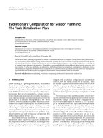
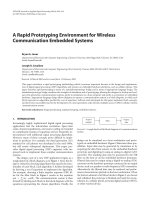
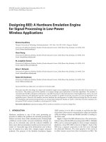
is typically random. LDPC codes can be effectively decoded
by the iterative belief-propagation (BP) algorithm [3] that,
as illustrated in Figure 1, directly matches the Tanner graph:
decoding messages are iteratively computed on each variable
node and check node and exchanged through the edges be-
tween the neighboring nodes.
Recently, tremendous efforts have been devoted to ana-
lyze and improve the LDPC codes error-correcting capabil-
ity, see [4, 5, 6, 7 , 8, 9, 10, 11] and so forth. Besides their
powerful error-correcting capability, another important rea-
son why LDPC codes attract so many attention is that the
iterative BP decoding algorithm is inherently fully parallel,
thus a great potential decoding speed can be expected.
The high-speed decoder hardware implementation is ob-
viously one of the most crucial issues determining the extent
of LDPC applications in the real world. The most natural so-
lution for the decoder architecture design is to directly in-

stantiate the BP decoding algorithm to hardware: each vari-
able node and check node are physically assigned their own
processors and all the processors are connected through an
interconnection network reflecting the Tanner graph con-
nectivity. By completely exploiting the parallelism of the BP
decoding algorithm, such fully parallel decoder can achieve
very high decoding speed, for example, a 1024-bit, rate-1/2
LDPC code fully parallel decoder with the maximum symbol
throughput of 1 Gbps has been physically implemented us-
ing ASIC technology [12]. The main disadvantage of such
An FPGA Implementation of (3, 6)-Regular LDPC Code Decoder 531
Check nodes
Variable n od es
Check-to-variable
message
Variable-to-check
message
Figure 1: Tanner graph representation of an LDPC code and the decoding messages flow.
fully parallel design is that with the increase of code length,
typically the LDPC code length is very large (at least several
thousands), the incurred hardware complexity will become
more and more prohibitive for many practical purposes,
for example, for 1-K code length, the ASIC decoder imple-
mentation [12]consumes1.7M gates. Moreover, as pointed
out in [12], the routing overhead for implementing the en-
tire interconnection network will become quite formidable
due to the large code length and randomness of the Tan-
ner graph. Thus high-speed partly parallel decoder de-
sign approaches that achieve appropriate trade-offsbetween
hardware complexity and decoding throughput are highly

desirable.
For any given LDPC code, due to the randomness of its
Tanner graph, it is nearly impossible to directly develop a
high-speed par tly parallel decoder architecture. To circum-
vent this difficulty, Boutillon et al. [13]proposedadecoder-
first code design methodology: instead of trying to conceive
the high-speed partly parallel decoder for any given ran-
dom LDPC code, use an available high-speed partly par-
allel decoder to define a constrained random LDPC code.
We may consider it as an application of the well-known
“Think in the reverse direction” methodology. Inspired by
the decoder-first code design methodology, we proposed
a joint code and decoder design methodology in [14]for
(3,k)-regular LDPC code partly parallel decoder design. By
jointly conceiving the code construction and partly paral-
lel decoder architecture design, we presented a (3,k)-regular
LDPC code partly parallel decoder structure in [14], which
not only defines very good (3,k)-regular LDPC codes but
also could potentially achieve high-speed partly parallel
decoding.
In this paper, applying the joint code and decoder design
methodology, we develop an elaborate (3,k)-regular LDPC
code high-speed partly parallel decoder architecture based
on which we implement a 9216-bit, rate-1/2(3, 6)-regular
LDPC code decoder using Xilinx Virtex FPGA (Field Pro-
grammable G ate Ar ray) de vice. In this work, we significantly
modify the original decoder structure [14] to improve the de-
coding throughput and simplify the control logic design. To
achieve good error-correcting capability, the LDPC code de-
coder architecture has to possess randomness to some extent,

which makes the FPGA implementations more challenging
since FPGA has fixed and regular hardware resources. We
propose a novel scheme to realize the random connectivity
by concatenating two routing networks, where all the ran-
dom hardwire routings are localized and the overall routing
complexity is significantly reduced. Exploiting the good min-
imum distance property of LDPC codes, this decoder em-
ploys parity check as the earlier decoding stopping criterion
to achieve adaptive decoding for energy reduction. With the
maximum 18 decoding iterations, this FPGA partly parallel
decoder supports a maximum of 54 Mbps symbol through-
put and achieves BER (bit error rate) 10
−6
at 2 dB over
AWGN channel.
This paper begins with a brief description of the LDPC
code decoding algorithm in Section 2.InSection 3,webriefly
describe the joint code and decoder design methodology for
(3,k)-regular LDPC code partly para llel decoder design. In
Section 4, we present the detailed high-speed partly parallel
decoder architecture design. Finally, an FPGA implementa-
tion of a (3, 6)-regular LDPC code partly parallel decoder is
discussed in Section 5.
2. DECODING ALGORITHM
Since the direct implementation of BP algorithm will incur
too high hardware complexity due to the large number of
multiplications, we introduce some logarithmic quantities
to convert these complicated multiplications into additions,
which lead to the Log-BP algorithm [2, 15].
Before the description of Log-BP decoding algorithm,

we introduce some definitions as follows. Let H denote the
M × N sparse parity-check matrix of the LDPC code and
H
i,j
denote the entry of H at the position (i, j). We de-
fine the set of bits n that participate in parity-check m as
ᏺ(m) ={n : H
m,n
= 1}, and the set of parity-checks m in
which bit n participates as ᏹ(n) ={m : H
m,n
= 1}.Wede-
note the set ᏺ(m) with bit n excluded by ᏺ(m) \ n, and the
set ᏹ(n) with parity-check m excluded by ᏹ(n) \ m.
Algorithm 1 (Iterative Log-BP Decoding Algorithm).
Input
The prior probabilities p
0
n
= P(x
n
= 0) and p
1
n
= P(x
n
= 1) =
1 − p
0
n

, n = 1, ,N;
Output
Hard decision x ={x
1
, ,x
N
};
Procedure
(1) Initialization: For each n, compute the intrinsic (or
channel) message γ
n
= log p
0
n
/p
1
n
and for each (m, n) ∈
532 EURASIP Journal on Applied Signal Processing
High-speed partly
parallel decoder
Random input H
3
Constrained random
parameters
Construction of

H =

H

1
H
2

Deterministic
input

H
(3,k)-regular LDPC code
ensemble defined by
H =


H
H
3

Selected code
Figure 2: Joint design flow diagram.
{(i, j) | H
i,j
= 1},compute
α
m,n
= sign

γ
n

log


1+e
−|γ
n
|
1 − e
−|γ
n
|

, (1)
where
sign

γ
n

=



+1,γ
n
≥ 0,
−1,γ
n
< 0.
(2)
(2) Iterative decoding
(i) Horizontal (or check node computation) step: for

each (m, n) ∈{(i, j) | H
i,j
= 1},compute
β
m,n
= log

1+e
−α
1 − e
−α


n

∈ᏺ(m)\n
sign

α
m,n


, (3)
where α =

n

∈ᏺ(m)\n
|α
m,n


|.
(ii) Vertical (or variable node computation) step: for
each (m, n) ∈{(i, j) | H
i,j
= 1},compute
α
m,n
= sign

γ
m,n

log

1+e
−|γ
m,n
|
1 − e
−|γ
m,n
|

, (4)
where γ
m,n
= γ
n
+


m

∈ᏹ(n)\m
β
m

,n
.Foreach
n, update the pseudoposterior log-likelihood ratio
(LLR) λ
n
as
λ
n
= γ
n
+

m∈ᏹ(n)
β
m,n
. (5)
(iii) Decision step:
(a) perform hard decision on {λ
1
, ,λ
N
} to ob-
tain x ={x

1
, ,x
N
} such that x
n
= 0 if
λ
n
> 0 and x
n
= 1 if λ ≤ 0;
(b) if H·x = 0, the n a lgorithm terminates, else go
to horizontal step until the preset maximum
number of iterations have occurred.
We cal l α
m,n
and β
m,n
in the above algorithm extrinsic
messages, where α
m,n
is delivered from variable node to check
node and β
m,n
is delivered from check node to variable node.
Each decoding iteration can be performed in fully paral-
lel fashion by physically mapping each check node to one in-
dividual check node processing unit (CNU) and each variable
node to one individual variable node processing unit (VNU).
Moreover, by delivering the hard decision x

i
from each VNU
to its neighboring CNUs, the parity-check H · x can be eas-
ily performed by all the CNUs. Thanks to the good min-
imum distance property of LDPC code, such adaptive de-
coding scheme can effectively reduce the average energy con-
sumption of the decoder without performance degradation.
In the partly parall el decoding, the operations of a cer-
tain number of check nodes or variable nodes are time-
multiplexed, or folded [16], to a single CNU or VNU. For
an LDPC code with M check nodes and N variable nodes, if
its partly parallel decoder contains M
p
CNUs and N
p
VNUs,
we denote M/M
p
as CNU folding factor and N/N
p
as VNU
folding factor.
3. JOINT CODE AND DECODER DESIGN
In this section, we briefly describe the joint (3,k)-regular
LDPC code and decoder design methodology [14]. It is well
known that the BP (or Log-BP) decoding algorithm works
well if the underlying Tanner graph is 4-cycle free and does
not contain too many short cycles. Thus the motivation of
this joint design approach is to construct an LDPC code that
not only fits to a high-speed partly parallel decoder but also

has the average cycle length as large as possible in its 4-cycle-
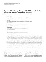
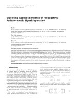
free Tanner graph. This joint design process is outlined as fol-
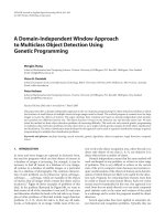
lows and the corresponding schematic flow diagram is shown
in Figure 2.
(1) Explicitly construct two matrices H
1
and H
2
in such a
way that

H = [H
T
1
, H
T
2
]
T
defines a (2,k)-regular LDPC
code C
2
whose Tanner graph has the girth
1
of 12.
(2) Develop a partly parallel decoder that is configured by
a set of constrained random parameters and defines
a(3,k)-regular LDPC code ensemble, in which each
code is a subcode of C
2

and has the parity-check matrix
H
= [

H
T
, H
T
3
]
T
.
(3) Select a good (3,k)-regular LDPC code from the code
ensemble based on the criteria of large Tanner graph
average cycle length and computer simulations. Typi-
cally the parity-check matrix of the selected code has
only few redundant checks, so we may assume that the
code rate is always 1 − 3/k.
1
Girth is the length of a shortest cycle in a graph.
An FPGA Implementation of (3, 6)-Regular LDPC Code Decoder 533

H=

H
1
H
2

=

L
I
1,1
I
2,1
.
.
.
I
k,1
I
1,2
I
2,2
.
.
.
I
k,2
00 0
···
I
1,k
I
2,k
.
.
.
I
k,k

0
0
0
P
1,1
P
2,1
···P
k,1
0
P
1,2
P
2,2
···
P
k,2
0
0
.
.
.
P
1,k
P
2,k
···
P
k,k
0

L · k
L · k
N = L · k
2
Figure 3: Structure of

H = [H
T
1
, H
T
2
]
T
.
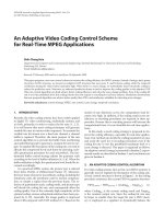
Construction of

H = [H
T
1
, H
T
2
]
T
The structure of

H is shown in Figure 3, where both H
1
and

H
2
are L · k by L · k
2
submatrices. Each block matrix I
x,y
in
H
1
is an L × L identity matrix and each block matrix P
x,y
in H
2
is obtained by a cyclic shift of an L × L identity ma-
trix. Let T denote the right cyclic shift operator where T
u
(Q)
represents right cyclic shifting matrix Q by u columns, then
P
x,y
= T
u
(I)whereu = ((x − 1) · y)modL and I represents
the L × L identity matrix, for example, if L = 5, x = 3, and
y = 4, we have u = (x − 1) · y mod L = 8mod5 = 3, then
P
3,4
= T
3
(I) =








00010
00001
10000
01000
00100







. (6)
Notice that in both H
1
and H
2
, each row contains k 1’s
and each column contains a single 1. Thus, the matrix

H =
[H
T

1
, H
T
2
]
T
defines a (2,k)-regular LDPC code C
2
with L ·
k
2
variable nodes and 2L · k check nodes. Let G denote the
Tanner graph of C
2
, we have the following theorem regarding
to the girth of G.
Theorem 1. If L cannot be factored as L = a · b,wherea, b ∈
{0, ,k− 1}, then the girth of G is 12 and there is at least one
12-cycle passing each check node.
Partly parallel decoder
Based on the specific structure of

H, a principal ( 3,k)-regular
LDPC code partly para llel decoder structure was presented in
[14]. This decoder is configured by a set of constrained ran-
dom parameters and defines a (3,k)-regular LDPC code en-
semble. Each code in this ensemble is essentially constructed
by inserting extra L · k check nodes to the high-gir th (2,k)-
regular LDPC code C
2

under the constraint specified by the
decoder. Therefore, it is reasonable to expect that the codes
in this ensemble more likely do not contain too many short
cycles and we may easily select a good code from it. For real
applications, we can select a good code from this code ensem-
ble as follows: first in the code ensemble, find several codes
with relatively high-average cycle lengths, then select the one
leading to the best result in the computer simulations.
The principal partly parallel decoder structure presented
in [14] has the following properties.
(i) It contains k
2
memory banks, each one consists of sev-
eral RAMs to store all the decoding messages associ-
ated with L variable nodes.
(ii) Each memory bank associates with one address gener-
ator that is configured by one element in a constrained
random integer set ᏾.
(iii) It contains a configurable random-like one-dimen-
sional shufflenetwork᏿ with the routing complexity
scaled by k
2
.
(iv) It contains k
2
VNUs and k CNUs so that the VNU and
CNU folding factors are L·k
2
/k
2

= L and 3L·k/k = 3L,
respectively.
(v) Each iteration completes in 3L clock cycles in which
only CNUs work in the first 2L clock cycles and both
CNUs and VNUs work in the last L clock cycles.
Over all the possible ᏾ and ᏿, this decoder defines a (3,k)-
regular LDPC code ensemble in which each code has the
parity-check matrix H = [

H
T
, H
T
3
]
T
, where the submatrix
H
3
is jointly specified by ᏾ and S.
4. PARTLY PARALLEL DECODER ARCHITECTURE
In this paper, applying the joint code and decoder design
methodology, we develop a high-speed (3,k)-regular LDPC
code partly parallel decoder architecture based on which a
9216-bit, rate-1/2(3, 6)-regular LDPC code partly parallel
decoder has been implemented using Xilinx Virtex FPGA
device. Compared with the structure presented in [14], this
partly parallel decoder architecture has the following distinct
characteristics.
(i) It employs a novel concatenated configurable ran-

dom two-dimensional shuffle network implementa-
tion scheme to realize the random-like connectivity
with low routing overhead, which is especially desir-
able for FPGA implementations.
(ii) To improve the decoding throughput, both the VNU
folding factor and CNU folding factor are L instead of
L and 3L in the structure presented in [14].
(iii) To simplify the control logic design and reduce the
memory bandwidth requirement, this decoder com-
pletes each decoding iteration in 2 L clock cycles in
which CNUs and VNUs work in the 1st and 2nd L
clock cycles, alternatively.
Following the joint design methodology, we have that this
decoder should define a (3,k)-regular LDPC code ensemble
in which each code has L
· k
2
variable nodes and 3L · k check
nodes and, as illustrated in Figure 4, the parity-check ma-
trix of each code has the form H = [H
T
1
, H
T
2
, H
T
3
]
T

where H
1
and H
2
have the explicit struc tures as shown in Figure 3 and
the random-like H
3
is specified by certain configuration pa-
rameters of the decoder. To facilitate the descr iption of the
534 EURASIP Journal on Applied Signal Processing
H=




H
1
H
2
H
3




=
Leftmost column
L
h
(k,2)

1
Rightmost column
h
(k,2)
L
I
1,1
.
.
.
I
k,1
I
1,2
.
.
.
I
k,2
···
I
1,k
.
.
.
I
k,k
L · k
P
1,1

···
P
k,1
P
1,2
···
P
k,2
.
.
.
P
1,k
···
P
k,k
L · k
L · k
H
(k,2)
L · k
2
Figure 4: The parity-check matrix.
decoder architecture, we introduce some definitions as fol-
lows: we denote the submatrix consisting of the L consecutive
columns in H that go through the block matrix I
x,y
as H
(x,y)
in which, from left to right, each column is labeled as h

(x,y)
i
with i increasing from 1 to L, a s shown in Figure 4.Welabel
the variable node corresponding to column h
(x,y)
i
as v
(x,y)
i
and
the L variable nodes v
(x,y)
i
for i = 1, ,Lconstitute a variable
node g roup VG
x,y
. Finally, we arrange the L · k check nodes
corresponding to all the L·k rows of submatrix H
i
into check
node group CG
i
.
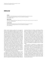
Figure 5 shows the principal structure of this partly par-
allel decoder. It mainly contains k
2
PE blocks PE
x,y
,for1≤ x
and y ≤ k, three bidirectional shufflenetworksπ

1
, π
2
,and
π
3
,and3· k CNUs. Each PE
x,y
contains one memory bank
RAMs
x,y
that stores all the decoding messages, including the
intrinsic and extrinsic messages and hard decisions, associ-
ated with all the L var iable nodes in the variable node group
VG
x,y
, and contains one VNU to perform the variable node
computations for these L variable nodes. Each bidirectional
shufflenetworkπ
i
realizes the extrinsic message exchange be-
tween all the L·k
2
variable nodes and the L·k check nodes in
CG
i
.Thek CNU
i,j
,forj = 1, ,k, perform the check node
computations for al l the L · k check nodes in CG

i
.
This decoder completes each decoding iteration in 2L
clock cycles, and during the first and second L clock cycles,
it works in check node processing mode and variable node
processing mode, respectively. In the check node processing
mode, the decoder not only performs the computations of
all the check nodes but also completes the extrinsic message
exchange between neighboring nodes. In variable node pro-
cessing mode, the decoder only performs the computations
of all the variable nodes.
The intrinsic and extrinsic messages are all quantized to
five bits and the iterative decoding datapaths of this partly
parallel decoder are illustrated in Figure 6, in which the dat-
apaths in check node processing and variable node process-
ing are represented by solid lines and dash dot lines, respec-
tively. As show n in Figure 6,eachPEblockPE
x,y
contains
five RAM blocks: EXT RAM i for i = 1, 2, 3, INT RAM, and
DEC RAM. Each EXT RAM i has L memory locations and
the location with the address d − 1(1≤ d ≤ L) contains
the extrinsic messages exchanged between the variable node
v
(x,y)
d
in VG
x,y
and its neighboring check node in CG
i

.The
INT RAM and DEC RAM store the intrinsic message and
hard decision associated with node v
(x,y)
d
at the memory lo-
cation with the address d − 1(1≤ d ≤ L). As we wil l see
later, such decoding messages storage strategy could greatly
simplify the control logic for generating the memory access
address.
For the purpose of simplicit y, in Figure 6 we do not show
the datapath from INT RAM to EXT RAM i’s for extrinsic
message initialization, which can be easily realized in L clock
cycles before the decoder enters the iterative decoding pro-
cess.
4.1. Check node processing
During the check node processing, the decoder performs the
computations of all the check nodes and realizes the extrinsic
message exchange between all the neighboring nodes. At the
beginning of check node processing, in each PE
x,y
the mem-
ory location with address d − 1inEXTRAM i contains 6-
bit hybrid data that consists of 1-bit hard decision and 5-bit
variable-to-check extrinsic message associated with the vari-
able node v
(x,y)
d
in VG
x,y

. In each clock cycle, this decoder
performs the read-shuffle-modify-unshuffle-write operations
to convert one variable-to-check extrinsic message in each
EXT RAM i to its check-to-variable counterpart. As illus-
trated in Figure 6, we may outline the datapath loop in check
node processing as follows:
(1) read:one6-bithybriddatah
(i)
x,y
is read from each
EXT RAM i in each PE
x,y
;
(2) shuffle:eachhybriddatah
(i)
x,y
goes through the shuffle
network π
i
and arrives at CNU
i,j
;
(3) modify:eachCNU
i,j
performs the parity check on the 6
input hard decision bits and generates the 6 output 5-
bit check-to-variable extrinsic messages β
(i)
x,y
based on

the 6 input 5-bit variable-to-check extrinsic messages;
(4) unshuffle: send each check-to-variable extr insic mes-
sage β
(i)
x,y
back to the PE block via the same path as its
variable-to-check counterpart;
(5) write:writeeachβ
(i)
x,y
to the same memory location in
EXT RAM i as its var iable-to-check counterpart.
All the CNUs deliver the parity-check results to a central
control block that will, at the end of check node processing,
determine whether all the parity-check equations specified
by the parity-check matrix have been satisfied, if yes, the de-
coding for current code frame will terminate.
To achieve higher decoding throughput, we implement
the read-shuffle-modify-unshuffle-write loop operation by
five-stage pipelining as show n in Figure 7, where CNU is
one-stage pip elined. To make this pipelining scheme feasi-
ble, we realize each bidirectional I/O connection in the three
An FPGA Implementation of (3, 6)-Regular LDPC Code Decoder 535
Active during
variable node processing
PE
1,1
VNU
RAMs
1,1

PE
2,1
VNU
RAMs
2,1
···
PE
k,k
VNU
RAMs
k,k
···
π
1
(regular & fixed)
···
π
2
(regular & fixed)
···
π
3
(random-like &
configurable)
CNU
1,1
···
CNU
1,k
CNU

2,1
···
CNU
2,k
CNU
3,1
···
CNU
3,k
Active during
check node processing
Figure 5: The principal (3,k)-regular LDPC code partly parallel decoder structure.
···
CNU
1,j
6bits
5bits
π
1
(regular & fixed)
h
(1)
x,y
···
CNU
2,j
6bits
5bits
π
2

(regular & fixed)
h
(2)
x,y
···
CNU
3,j
6bits
5bits
π
3
(random-like &
configurable)
h
(3)
x,y
PE
x,y
{h
(i)
x,y
} 18 bits
{β
(i)
x,y
}
15 bits
EXT RAM 1
EXT RAM 2
EXT RAM 3

18 bits
{h
(i)
x,y
}
{β
(i)
x,y
}
15 bits
INT RAM
5bits
VNU
1bit
DEC RAM
Figure 6: Iterative decoding datapaths.
CNU
Read
6bits
Shuffle
6bits
CNU
(1st half)
CNU
(2nd half)
5bits
Unshuffle
5bits
Write
Figure 7: Five-stage pipelining of the check node processing datapath.

shuffle networks by two distinct sets of wires with opposite
directions, which means that the hybrid data from PE blocks
to CNUs and the check-to-variable extrinsic messages from
CNUs to PE blocks are carried on distinct sets of wires. Com-
pared with sharing one set of wires in time-multiplexed fash-
ion, this approach has higher wire routing overhead but ob-
viates the logic gate overhead due to the realization of t ime-
multiplex and, more importantly, make it feasible to directly
pipeline the datapath loop for higher decoding throughput.
In this decoder, one address generator AG
(i)
x,y
associates
with one EXT RAM i in each PE
x,y
. In the check node pro-
cessing, AG
(i)
x,y
generates the address for reading hybrid data
and, due to the five-stage pipelining of datapath loop, the ad-
dress for writing back the check-to-variable message is ob-
tained via delaying the read address by five clock cycles. It
is clear that the connectivity among all the variable nodes
and check nodes, or the entire parity-check matrix, realized
by this decoder is jointly specified by all the address genera-
tors and the three shufflenetworks.Moreover,fori = 1, 2, 3,
the connectivity among all the var iable nodes and the check
nodes in CG
i

is completely determined by AG
(i)
x,y
and π
i
.Fol-
lowing the joint design methodology, we implement all the
address generators and the three shufflenetworksasfollows.
4.1.1 Implementations of AG
(1)
x,y
and π
1
The bidirectional shufflenetworkπ
1
and AG
(1)
x,y
realize the
connectivity among all the variable nodes and all the check
nodes in CG
1
as specified by the fixed submatr ix H
1
.Recall
536 EURASIP Journal on Applied Signal Processing
π
3
Input data
from PE blocks

a
1,1
···
a
1,k
.
.
.
a
k,1
···
a
k,k
.
.
.
.
.
.
r = 0 ···L − 1
ROM
R
s
(r)
1
a
1,1
···
a
1,k

Ψ
(r)
1
(R
1
or Id)
1bit
b
1,1
b
1,k
···
.
.
.
1bit
s
(r)
k
a
k,1
···
a
k,k
Ψ
(r)
k
(R
k
or Id)

b
k,1
··· b
k,k
Stage I: intrarow shuffle
r = 0 ···L − 1
ROM
C
1bit
s
(c)
1
b
1,1
.
.
.
b
k,1
Ψ
(c)
1
(C
1
or Id)
c
1,1
.
.
.

c
k,1
1bit
s
(c)
k
b
1,1
.
.
.
···
b
k,1
Ψ
(c)
k
(C
k
or Id)
c
1,1
.
.
.
c
k,1
Output data
to CNU
3,j

’s
c
1,1
···
c
1,k
.
.
.
.
.
.
.
.
.
c
k,1
···
c
k,k
Stage II: intracolumn shuffle
Figure 8: Forward path of π
3
.
that node v
(x,y)
d
corresponds to the column h
(x,y)
i

as illustrated
in Figure 4 and the extrinsic messages associated with node
v
(x,y)
d
are always stored at address d − 1. Exploiting the ex-
plicit structure of H
1
, we easily obtain the implementation
schemes for AG
(1)
x,y
and π
1
as follows:
(i) each AG
(1)
x,y
is realized as a log
2
L-bit binary counter
that is cleared to zero at the beginning of check node
processing;
(ii) the bidirectional shufflenetworkπ
1
connects the k
PE
x,y
with the same x-index to the same CNU.
4.1.2 Implementations of AG

(2)
x,y
and π
2
The bidirectional shufflenetworkπ
2
and AG
(2)
x,y
realize the
connectivity among all the variable nodes and all the check
nodes in CG
2
as specified by the fixed matrix H
2
. Similarly,
exploiting the extrinsic messages storage strategy and the ex-
plicit structure of H
2
, we implement AG
(2)
x,y
and π
2
as follows:
(i) each AG
(2)
x,y
is realized as a log
2

L-bit binary counter
that only counts up to the value L − 1 and is loaded
with the value of ((x − 1) · y)modL at the beginning
of check node processing;
(ii) the bidirectional shufflenetworkπ
2
connects the k
PE
x,y
with the same y-index to the same CNU.
Notice that the counter load value for each AG
(2)
x,y
directly
comes from the construction of each block matrix P
x,y
in H
2
as descr ibed in Section 3.
4.1.3 Implementations of AG
(3)
x,y
and π
3
The bidirectional shufflenetworkπ
3
and AG
(3)
x,y
jointly de-

fine the connectivity among all the variable nodes and all the
check nodes in CG
3
, which is represented by H
3
as illustrated
in Figure 4. In the above, we show that by exploiting the spe-
cific structures of H
1
and H
2
and the extrinsic messages stor-
age strategy, we can directly obtain the implementations of
each AG
(i)
x,y
and π
i
,fori = 1, 2. However, the implementa-
tions of AG
(3)
x,y
and π
3
are not easy because of the following
requirements on H
3
:
(1) the Tanner graph corresponding to the parity-check
matrix H = [H

T
1
, H
T
2
, H
T
3
]
T
should be 4-cycle free;
(2) to make H random to some extent, H
3
should be
random-like.
As proposed in [14], to simplify the design process, we
separately conceive AG
(3)
x,y
and π
3
in such a way that the im-
plementations of AG
(3)
x,y
and π
3
accomplish the above first and
second requirements, respectively.
Implementations of AG

(3)
x,y
We implement each AG
(3)
x,y
as a log
2
L-bit binary counter
that counts up to the value L − 1 and is initialized with a
constant value t
x,y
at the beginning of check node process-
ing. Each t
x,y
is selected in random under the following two
constraints:
(1) given x, t
x,y
1
= t
x,y
2
,forally
1
,y
2
∈{1, ,k};
(2) given y, t
x
1

,y
− t
x
2
,y
≡ ((x
1
− x
2
) · y)modL,forall
x
1
,x
2
∈{1, ,k}.
It can be proved that the above two constraints on t
x,y
are
sufficient to make the entire parity-check matrix H always
correspond to a 4-cycle free Tanner graph no matter how we
implement π
3
.
Implementation of π
3
Since each AG
(3)
x,y
is realized as a counter, the pattern of shuf-
fle network π

3
cannot be fixed, otherwise the shufflepattern
of π
3
will be regularly repeated in the H
3
, which means that
H
3
will always contain very regular connectivity patterns no
matter how random-like the pattern of π
3
itself is. Thus we
should make π
3
configurable to some extent. In this paper,
we propose the following concatenated configurable random
shuffle network implementation scheme for π
3
.
Figure 8 shows the forward path (from PE
x,y
to CNU
3,j
)
of the bidirectional shufflenetworkπ
3
. In each clock cycle, it
An FPGA Implementation of (3, 6)-Regular LDPC Code Decoder 537
realizes the data shufflefroma

x,y
to c
x,y
by two concatenated
stages: intrarow shuffleandintracolumn shuffle. Firstly, the
a
x,y
data block, where each a
x,y
comes from PE
x,y
, passes an
intrarow shuffle network array in which each shufflenetwork
Ψ
(r)
x
shuffles the k input data a
x,y
to b
x,y
for 1 ≤ y ≤ k.Each
Ψ
(r)
x
is configured by 1-bit control signal s
(r)
x
leading to the
fixed random permutation R
x

if s
(r)
x
= 1, or to the identity
permutation (Id) otherwise. The reason why we use the Id
pattern instead of another random shuffle pattern is to min-
imize the routing overhead, and our simulations suggest that
there is no gain on the error-correcting performance by using
another random shuffle pattern instead of Id pattern. The k-
bit configuration word s
(r)
changes every clock cycle and all
the Lk-bit control words are stored in ROM R. Next, the b
x,y
data block goes through an intracolumn shufflenetworkar-
ray in which each Ψ
(c)
y
shuffles the kb
x,y
to c
x,y
for 1 ≤ x ≤ k.
Similarly, each Ψ
(c)
y
is configured by 1-bit control signal s
(c)
y
leading to the fixed random p ermutation C

y
if s
(c)
y
= 1, or to
Id otherwise. The k-bit configuration word s
(c)
y
changes ev-
ery clock cycle and all the Lk-bit control words are stored
in ROM C. As the output of forward path, the kc
x,y
with the
same x-index are delivered to the same CNU
3,j
. To realize the
bidirectional shuffle, we only need to implement each config-
urable shufflenetworkΨ
(r)
x
and Ψ
(c)
y
as bidirectional so that
π
3
can unshuffle the k
2
data backward from CNU
3,j

to PE
x,y
along the same route as the forward path on distinct sets of
wires. Notice that, due to the pipelining on the datapath loop,
the backward path control signals are obtained via delaying
the forward path control signals by three clock cycles.
To make the connectivity realized by π
3
random-like and
change each clock cycle, we only need to randomly generate
the control words s
(r)
x
and s
(c)
y
for each clock cycle and the
fixed shufflepatternsofeachR
x
and C
y
. Since most modern
FPGA devices have multiple metal layers, the implementa-
tions of the two shuffle arrays can be overlapped from the
bird’s-eye view. Therefore, the above concatenated imple-
mentation scheme will confine all the routing wires to small
area (in one row or one column), which will significantly
reduce the possibility of routing congestion and reduce the
routing overhead.
4.2. Variable node processing

Compared with the above check node processing, the opera-
tions performed in the variable node processing is quite sim-
ple since the decoder only needs to carry out all the variable
node computations. Notice that at the beginning of variable
node processing, the three 5-bit check-to-variable extrinsic
messages associated with each variable node v
(x,y)
d
are stored
at the address d − 1 of the three EXT RAM i in PE
x,y
.The
5-bit intrinsic message associated with variable node v
(x,y)
d
is
also stored at the address d −1ofINT RAM in PE
x,y
.Ineach
clock cycle, this decoder performs the read-modify-write op-
erations to convert the three check-to-variable extrinsic mes-
sages associated with the same variable node to three hybrid
data consisting of variable-to-check extrinsic messages and
VNU
Read
5bits
VNU
(1st half)
VNU
(2nd half)

6bits
1bit
Write
Figure 9: Three-stage pipelining of the variable node processing
datapath.
hard decisions. As shown in Figure 6, we may outline the dat-
apath loop in variable node processing as follows:
(1) read:ineachPE
x,y
, three 5-bit check-to-variable ex-
trinsic messages β
(i)
x,y
and one 5-bit intrinsic messages
γ
x,y
associated with the same variable node are read
from the three EXT RAM i and INT RAM at the same
address;
(2) modify: based on the input check-to-variable extrinsic
messages and intrinsic message, each VNU generates
the 1-bit hard decision
x
x,y
and three 6-bit hybrid data
h
(i)
x,y
;
(3) write:eachh

(i)
x,y
is written back to the same memory
location as its check-to-variable counterpart and x
x,y
is written to DEC RAM.
The forward path from memory to VNU and backward
path from VNU to memory are implemented by distinct sets
of w ires and the entire read-modify-write datapath loop is
pipelined by three-stage pipelining as illustrated in Figure 9.
Since all the extrinsic and intrinsic messages associated
with the same variable node are stored at the same address
in different RAM blocks, we can use only one binary counter
to generate all the read address. Due to the pipelining of the
datapath, the write address is obtained via delaying the read
address by three clock cycles.
4.3. CNU and VNU architectures
Each CNU carries out the operations of one check node,
including the parity check and computation of check-to-
variable extrinsic messages. Figure 10 shows the CNU archi-
tecture for check node with the degree of 6. Each input x
(i)
is a 6-bit hybrid data consisting of 1-bit hard decision and
5-bit variable-to-check extrinsic message. The parity check is
performed by XORing all the six 1-bit hard decisions. Each
5-bit variable-to-check extrinsic messages is represented by
sign-magnitude format with a sign bit and four magnitude
bits. The architecture for computing the check-to-variable
extrinsic messages is directly obtained from (3). The func-
tion f (x) = log((1 + e

−|x|
)/(1 − e
−|x|
)) is realized by the LUT
(lookup table) that is implemented as a combinational logic
block in FPGA. Each output 5-bit check-to-variable extrinsic
message y
(i)
is also represented by sign-magnitude format.
Each VNU generates the hard decision and all the
variable-to-check extrinsic messages associated with one
variable node. Figure 11 shows the VNU architecture for
variable node with the degree of 3. With the input 5-bit in-
trinsic message z and three 5-bit check-to-variable extrinsic
messages y
(i)
associated with the same variable node, VNU
538 EURASIP Journal on Applied Signal Processing
X
(1)
6
51
X
(2)
6
51
X
(3)
6
51

X
(4)
6
51
X
(5)
6
51
X
(6)
6
51
41 41 41 41 41 41
6
LUT
6
LUT
6
LUT
6
LUT
6
LUT
6
LUT
41
5
y
(1)
41

5
y
(2)
41
5
y
(3)
41
5
y
(4)
41
5
y
(5)
41
5
y
(6)
Pipeline
1
Parity-check result
Figure 10: Architecture for CNU with k = 6.
Z
5
Pipeline
S-to-T: Sign magnitude to two’s complement
T-to-S: Two’s complement to sign-magnitude
1
Hard decision

y
(1)
5
S-to-T
y
(2)
5
S-to-T
y
(3)
5
S-to-T
T-to-S
76
LUT
4
1
6
X
(1)
T-to-S
76
LUT
4
1
6
X
(2)
T-to-S
7

6
LUT
4
1
6
X
(3)
Figure 11: Architecture for VNU with j = 3.
generates three 5-bit variable-to-check extrinsic messages
and 1-bit hard decision according to (4)and(5), respectively.
To enable each CNU to receive the hard decisions to per-
form parity check as described above, the hard decision is
combined with each 5-bit variable-to-check extrinsic mes-
sage to form 6-bit hybrid data x
(i)
as shown in Figure 11.
Since each input check-to-variable extrinsic message y
(i)
is
represented by s ign-magnitude format, we need to convert
it to two’s complement format before performing the addi-
tions. Before going through the LUT that realizes f (x) =
log((1 + e
−|x|
)/(1 − e
−|x|
)), each data is converted back to the
sign-magnitude format.
4.4. Data Input/Output
This partly parallel decoder works simultaneously on three

consecutive code frames in two-stage pipelining mode: while
one frame is being iteratively decoded, the next frame is
loaded into the decoder, and the hard decisions of the
previous frame are read out from the decoder. Thus each
INT RAM contains two RAM blocks to store the intrinsic
messages of both current and next frames. Similarly, each
DEC RAM contains two RAM blocks to store the hard de-
cisionsofbothcurrentandpreviousframes.
The design scheme for intrinsic message input and hard
decision output is heavily dependent on the floor planning of
An FPGA Implementation of (3, 6)-Regular LDPC Code Decoder 539
Intrinsic
data
5
Load
address
log
2
L + log
2
k
2

log
2
L
log
2
k
2


Binary decoder
k
2
PE block
select
log
2
L
Read
address
PE
1,1
1
PE
1,2
2
PE
2,1
1
PE
2,2
2
.
.
.
.
.
.
PE

k,1
1
PE
k,2
2
···
···
···
···
k − 1
PE
1,k
k
k − 1
PE
2,k
k
.
.
.
k − 1
PE
k,k
k
k
2
Decoding
output
Figure 12: Data input/output structure.
the k

2
PE blocks. To minimize the routing overhead, we de-
velop a square-shaped floor planning for PE blocks as illus-
trated in Figure 12 and the corresponding data input/output
scheme is described in the following.
(1) Intrinsic data input. The intrinsic messages of next
frame is loaded, 1 symbol per clock cycle. As shown
in Figure 12, the memory location of each input in-
trinsic data is determined by the input load ad-
dress that has the width of (log
2
L + log
2
k
2
)bits
in which log
2
k
2
 bits specify w hich PE block (or
which INT RAM) is being accessed and the other
log
2
L bits locate the memory location in the selected
INT RAM. As shown in Figure 12, the primary intrin-
sic data and load address input directly connect to the
k PE blocks PE
1,y
for 1 ≤ y ≤ k,andfromeachPE

x,y
the intrinsic data and load address are delivered to the
adjacent PE block PE
x+1,y
in pipelined fashion.
(2) Decoded data output. The decoded data (or hard deci-
sions) of the previous frame is read out in pipelined
fashion. As shown in Figure 12, the primary log
2
L-
bit read address input directly connects to the k PE
blocks PE
x,1
for 1 ≤ x ≤ k,andfromeachPE
x,y
the
read address are delivered to the adjacent block PE
x,y+1
in pipelined fashion. Based on its input read address,
each PE block outputs 1-bit hard decision per clock
cycle. Therefore, as illustrated in Figure 12, the width
of pipelined decoded data bus increases by 1 after go-
ing through one PE block, and at the rightmost side,
we obtain kk-bit decoded output that are combined
together as the k
2
-bit primary decoded data output.
5. FPGA IMPLEMENTATION
Applying the above decoder architecture, we implemented
a(3,6)-regular LDPC code partly parallel decoder for L =

256 using Xilinx Virtex-E XCV2600E device with the pack-
age FG1156. The corresponding LDPC code length is N =
L · k
2
= 256 · 6
2
= 9216 and code rate is 1/2. We obtain
the constrained random parameter set for implementing π
3
and each AG
(3)
x,y
as follows: first generate a large number of
parameter sets from which we find few sets leading to rela-
tively high Tanner graph average cycle length, then we select
one set leading to the best performance based on computer
simulations.
The target XCV2600E FPGA device contains 184 large
on-chip block RAMs, each one is a fully synchronous dual-
port 4K-bit RAM. In this decoder implementation, we con-
figure each dual-port 4K-bit RAM as two independent
single-port 256 × 8-bit RAM blocks so that each EXT RAM i
can be realized by one single-port 256 × 8-bit RAM block.
Since each INT RAM contains two RAM blocks for storing
the intrinsic messages of both current and next code frames,
we use two single-port 256 × 8-bit RAM blocks to imple-
ment one INT RAM. Due to the relatively small memory size
requirement, the DEC RAM is realized by distributed RAM
that provides shallow RAM structures implemented in CLBs.
Since this decoder contains k

2
= 36 PE blocks, each one in-
corporates one INT RAM and three EXT RAM i’s, we to-
tally utilize 180 single-port 256 × 8-bit RAM blocks (or 90
dual-port 4K-bit RAM blocks). We manually configured the
placement of each PE block according to the floor-planning
scheme as shown in Figure 12. Notice that such placement
540 EURASIP Journal on Applied Signal Processing
Table 1: FPGA resources utilization statistics.
Resource Number Utilization rate Resource Number Utilization rate
Slices 11,792 46% Slices Registers 10,105 19%
4 input LUTs 15,933 31% Bonded IOBs 68 8%
Block RAMs 90 48% DLLs 1 12%
PE
1,1
PE
2,1
PE
3,1
PE
4,1
PE
5,1
PE
6,1
PE
1,2
PE
2,2
PE

3,2
PE
4,2
PE
5,2
PE
6,2
PE
1,3
PE
2,3
PE
3,3
PE
4,3
PE
5,3
PE
6,3
PE
1,4
PE
2,4
PE
3,4
PE
4,4
PE
5,4
PE

6,4
PE
1,5
PE
2,5
PE
3,5
PE
4,5
PE
5,5
PE
6,5
PE
1,6
PE
2,6
PE
3,6
PE
4,6
PE
5,6
PE
6,6
Figure 13: The placed and routed decoder i mplementation.
scheme exactly matches the structure of the configurable
shufflenetworkπ
3
as described in Section 4.1.3, thus the

routing overhead for implementing the π
3
is also minimized
in this FPGA implementation.
From the architecture description in Section 4, we know
that, during each clock cycle in the iterative decoding, this
decoder need to perform both read and write operations on
each single-port RAM block EXT RAM i. Therefore, sup-
pose the primary clock frequency is W, we must generate
a2× W clock signal as the RAM control signal to achieve
read-and-write operation in one clock cycle. This 2 × W
clock signal is gener ated using the delay-locked loop (DLL)
in XCV2600E.
To facilitate the entire implementation process, we exten-
sively utilized the highly optimized Xilinx IP cores to instan-
tiate many function blocks, that is, all the RAM blocks, all
the counters for generating addresses, and the ROMs used to
store the control signals for shufflenetworkπ
3
.Moreover,all
the adders in CNUs and VNUs are implemented by ripple-
carry adder that is exactly suitable for Xilinx FPGA imple-
mentations thanks to the on-chip dedicated fast arithmetic
carry chain.
This decoder was described in the VHDL (hardware de-
scription language) and SYNOPSYS FPGA Express was used
to synthesize the VHDL implementation. We used the Xil-
inx Development System tool suite to place and route the
synthesized implementation for the target XCV2600E device
with the speed option −7. Tabl e 1 shows the hardware re-

source utilization statistics. Notice that 74% of the total uti-
lized slices, or 8691 slices, were used for implementing all
the CNUs and VNUs. Figure 13 shows the placed and routed
design in which the placement of all the PE blocks are con-
strained based on the on-chip RAM block locations.
Based on the results reported by the Xilinx static timing
analysis tool, the maximum decoder clock frequency can be
56 MHz. If this decoder performs s decoding iterations for
each code frame, the total clock cycle number for decoding
one frame will be 2s
· L + L, where the extra L clock cycles
is due to the initialization process, and the maximum sym-
bol decoding throughput will be 56 · k
2
· L/(2s · L + L) =
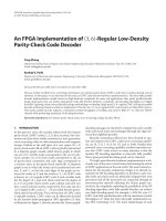
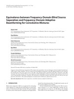
56·36/(2s+1)Mbps. Here,we set s = 18 and obtain the max-
imum symbol decoding throughput as 54 Mbps. Figure 14
shows the corresponding performance over AWGN channel
with s = 18, including the BER, FER (frame error rate), and
the average iteration numbers.
6. CONCLUSION
Due to the unique characteristics of LDPC codes, we be-
lieve that jointly conceiving the code construction and
partly parallel decoder design should be a key for practi-
cal high-speed LDPC coding system implementations. In
this paper, applying a joint design methodology, we devel-
oped a (3,k)-regular LDPC code high-speed partly paral-
lel decoder architecture design and implemented a 9216-
bit, rate-1/2(3, 6)-regular LDPC code decoder on the Xil-
inx XCV2600E FPGA device. The detailed decoder architec-

ture and floor planning scheme have been presented and a
concatenated configurable random shuffle network imple-
mentation is proposed to minimize the routing overhead
for the random-like shuffle network realization. With the
maximum 18 decoding iterations, this decoder can achieve
up to 54 Mbps symbol decoding throughput and the BER
10
−6
at 2 dB over AWGN channel. Moreover, exploiting
the good minimum distance property of LDPC code, this
decoder uses parity check after each iteration as earlier
stopping criterion to effectively reduce the average energy
consumption.
An FPGA Implementation of (3, 6)-Regular LDPC Code Decoder 541
10
0
10
−1
10
−2
10
−3
10
−4
10
−5
10
−6
BER/FER
11.522.5

E
b
/N
0
(dB)
BER
FER
18
16
14
12
10
8
6
4
Average number of iterations
11.522.533.5
E
b
/N
0
(dB)
Figure 14: Simulation results on BER, FER and the average itera-
tion numbers.
REFERENCES
[1] R. G. Gallager, “Low-density parity-check codes,” IRE Trans-
actions on Information Theory, vol. IT-8, no. 1, pp. 21–28,
1962.
[2] R.G.Gallager, Low-Density Parity-Check Codes, MIT Press,
Cambridge, Mass, USA, 1963.

[3] D. J. C. MacKay, “Good error-correcting codes based on very
sparse matrices,” IEEE Transactions on Information Theory,
vol. 45, no. 2, pp. 399–431, 1999.
[4] M.C.DaveyandD.J.C.MacKay, “Low-densityparitycheck
codes over GF(q),” IEEE Communications Letters, vol. 2, no.
6, pp. 165–167, 1998.
[5] M. Luby, M. Mitzenmacher, M. Shokrollahi, and D. Spiel-
man, “Improved low-density parity-check codes using irregu-
lar graphs and belief propagation,” i n Proc. IEEE International
Symposium on Information Theory, p. 117, Cambridge, Mass,
USA, August 1998.
[6] T. Richardson and R. Urbanke, “The capacity of low-density
parity-check codes under message-passing decoding,” IEEE
Transactions on Information Theory, vol. 47, no. 2, pp. 599–
618, 2001.
[7] T. Richardson, M. Shokrollahi, and R. Urbanke, “Design
of capacity-approaching irregular low-density parity-check
codes,” IEEE Transactions on Information Theory, vol. 47, no.
2, pp. 619–637, 2001.
[8] S Y. Chung, T. Richardson, and R. Urbanke, “Analysis of
sum-product decoding of low-density parity-check codes us-
ing a Gaussian approximation,” IEEE Transactions on Infor-
mation Theory, vol. 47, no. 2, pp. 657–670, 2001.
[9] M. Luby, M. Mitzenmacher, M. Shokrollahi, and D. A. Spiel-
man, “Improved low-density parity-check codes using irreg-
ular graphs,” IEEE Transactions on Information Theory, vol.
47, no. 2, pp. 585–598, 2001.
[10] S Y. Chung, G. D. Forney, T. Richardson, and R. Urbanke,
“On the design of low-density parity-check codes within
0.0045 dB of the Shannon limit,” IEEE Communications Let-

ters, vol. 5, no. 2, pp. 58–60, 2001.
[11] G. Miller and D. Burshtein, “Bounds on the maximum-
likelihood decoding error probability of low-density parity-
check codes,” IEEE Transactions on Information Theory, vol.
47, no. 7, pp. 2696–2710, 2001.
[12] A. J. Blanksby and C. J. Howland, “A 690-mW 1-Gb/s 1024-b,
rate-1/2 low-density parity-check code decoder,” IEEE Journal
of Solid-State Circuits, vol. 37, no. 3, pp. 404–412, 2002.
[13] E. Boutillon, J. Castura, and F. R. Kschischang, “Decoder-
first code design,” in Proc. 2nd International Symposium on
Turbo Codes and Related Topics, pp. 459–462, Brest, France,
September 2000.
[14] T. Zhang and K. K. Parhi, “VLSI implementation-oriented
(3,k)-regular low-density parity-check codes,” in IEEE Work-
shop on Signal Processing Systems (SiPS), pp. 25–36, Antwerp,
Belgium, September 2001.
[15] M. Chiani, A. Conti, and A. Ventura, “Evaluation of low-
density parity-check codes over block fading channels,” in
Proc. IEEE International Conference on Communications,pp.
1183–1187, New Orleans, La, USA, June 2000.
[16] K. K. Parhi, VLSI Digital Signal Processing Systems: Design and
Implementation, John Wiley & Sons, New York, USA, 1999.
Tong Zhang received his B.S. and M.S.
degrees in electrical engineering from the
Xian Jiaotong University, Xian, China, in
1995 and 1998, respectively. He received the
Ph.D. degree in electrical engineering from
the University of Minnesota in 2002. Cur-
rently, he is an Assistant Professor in Elec-
trical, Computer, and Systems Engineering

Department at Rensselaer Polytechnic Insti-
tute. His current research interests include
design of VLSI architectures and circuits for digital signal pro-
cessing and communication systems, with the emphasis on error-
correcting coding and multimedia processing.
542 EURASIP Journal on Applied Signal Processing
Keshab K. Parhi is a Distinguished McK-
night University Professor in the Depart-
ment of Electrical and Computer Engineer-
ing at the University of Minnesota, Min-
neapolis. He was a Visiting Professor at
Delft University and Lund University, a
Visiting Researcher at NEC Corporation,
Japan, (as a National Science Foundation
Japan Fellow), and a Technical Director DSP
SystemsatBroadcomCorp.Dr.Parhi’sre-
search interests have spanned the areas of VLSI architectures for
digital signal and image processing, adaptive digital filters and
equalizers, error control coders, cryptography architectures, high-
level architecture transformations and synthesis, low-power digital
systems, and computer arithmetic. He has published over 350 pa-
pers in these areas, authored the widely used textbook VLSI Digital
Signal Processing Systems (Wiley, 1999) and coedited the reference
book Digital Signal Processing for Multimedia Digital Sig nal Process-
ing Systems (Wiley, 1999). He has received numerous best paper
awards including the most recent 2001 IEEE WRG Baker Prize Pa-
per Award. He is a Fellow of IEEE, and the recipient of a Golden
Jubilee medal from the IEEE Circuits and Systems Society in 1999.
He is the recipient of the 2003 IEEE Kiyo Tomiyasu Technical Field
Award.