EURASIP Journal on Applied Signal Processing 2003:8, 841–859 c 2003 Hindawi Publishing doc

EURASIP Journal on Applied Signal Processing 2003:8, 841–859
c
 2003 Hindawi Publishing Corporation
A Domain-Independent Window Approach
to Multiclass Object Detection Using
Genetic Programming
Mengjie Zhang
School of Mathematical and Computing Sciences, Victoria University of Wellington, P.O. Box 600, Wellington, New Zealand
Email:
Victor B. Ciesielski
School of Computer Science and Information Technology, RMIT University, GPO Box 2476v Melbourne, 3001 Victoria, Australia
Email:
Peter Andreae
School of Mathematical and Computing Sciences, Victoria University of Wellington, P.O. Box 600, Wellington, New Zealand
Email:
Received 30 June 2002 and in revis ed form 7 March 2003
This paper describes a domain-independent approach to the use of genetic programming for object detection problems in which
the locations of small objects of multiple classes in large images must be found. The evolved program is scanned over the large
images to locate the objects of interest. The paper develops three terminal sets based on domain-independent pixel statistics
and considers two different function sets. The fitness function is based on the detection rate and the false alarm rate. We have
tested the method on three object detection problems of increasing difficulty. This work not only extends genetic programming
to multiclass-object detection problems, but also shows how to use a single evolved genetic program for both object classification
and localisation. The object classification map developed in this approach can be used as a general classification strategy in genetic
programming for multiple-class classification problems.
Keywords and phrases: machine learning, neural networks, genetic algorithms, object recognition, target detection, computer
vision.
1. INTRODUCTION
As more and more images are captured in electronic form,
the need for programs which can find objects of interest in
a database of images is increasing. For example, it may be
necessary to find all tumors in a database of x-ray images,

all cyclones in a database of satellite images, or a particular
face in a database of photographs. The common character-
isticofsuchproblemscanbephrasedas“givensubimage
1
,
subimage
2
, , subimage
n
which are examples of the objects
of interest, find all images which contain this object and its
location(s).” Figure 10 shows examples of problems of this
kind. In the problem illustr ated by Figure 10b,wewantto
find centers of all of the Australian 5-cent and 20-cent coins
and determine whether the head or the tail side is up. Exam-
ples of other problems of this kind include target detection
problems [1, 2, 3], where the task is to find, say, all tanks,
trucks, or helicopters in an image. Unlike most of the cur-
rent work in the object recognition area, where the task is to
detect only objects of one class [1, 4, 5], our objective is to
detect objects from a number of classes.
Domain independence means that the same method will
work unchanged on any problem, or at least on some range
of problems. This is very difficult to achieve at the current
state of the art in computer vision because most systems re-
quire careful analysis of the objects of interest and a determi-
nation of which features are likely to be useful for the detec-
tion task. Programs for extrac ting these features must then
be coded or found in some feature librar y. Each new vision
system must be handcrafted in this way. Our approach is to

work from the raw pixels directly or to use easily computed
pixel statistics such as the mean and variance of the pixels
in a subimage and to evolve the programs needed for object
detection.
Several approaches have been applied to automatic ob-
ject detection and recognition problems. Typically, they use
842 EURASIP Journal on Applied Signal Processing
multiple independent stages, such as preprocessing, edge de-
tection, segmentation, feature extraction, and object classifi-
cation [6, 7], which often results in some efficiency and effec-
tiveness problems. The final results rely too much upon the
results of earlier stages. If some objects are lost in one of the
early stages, it is very difficult or impossible to recover them
in the later stage. To avoid these disadvantages, this paper in-
troduces a single-stage approach.
There have been a number of reports on the use of ge-
netic programming (GP) in object detection and classifica-
tion [8, 9]. Winkeler and Manjunath [10]describeaGP
system for object detection in which the evolved functions
operate directly on the pixel values. Teller and Veloso [11]
describe a GP system and a face recognition application in
which the evolved programs have a local indexed memory.
All of these approaches are based on detecting one class of
objects or two-class classification problems, that is, objects
versus everything else. GP naturally lends itself to binary
problems as a program output of less than 0 can be inter-
preted as one class and greater than or equal to 0 as the other
class. It is not obvious how to use GP for more than two
classes. The approach in this paper will focus on object de-
tection problems in which a number of objects in more than

two classes of interest need to be localised and classified.
1.1. Outline of the approach to object detec tion
A brief outline of the method is as follows.
(1) Assemble a database of images in which the locations
and classes of all of the objects of interest are manually
determined. Split these images into a training set and
atestset.
(2) Determine an appropriate size (n × n)ofasquare
which will cover all single objects of interest to form
the input field.
(3) Invoke an evolutionary process with images in the
training set to generate a program which can deter-
mine the class of an object in its input field.
(4) Apply the generated program as a moving window
template to the images in the test set and obtain the
locations of all the objects of interest in each class. Cal-
culate the detection rate (DR) and the false alarm rate
(FAR) on the test set as the measure of performance.
1.2. Goals
The overall goal of this paper is to investigate a learn-
ing/adaptive, single-stage, and domain-independent ap-
proach to multiple-class object detection problems without
any preprocessing, segmentation, and specific feature extrac-
tion. This approach is based on a GP technique. Rather
than using specific image features, pixel statistics are used
as inputs to the evolved programs. Specifically, the following
questionswillbeexploredonasequenceofdetectionprob-
lems of increasing difficulty to determine the strengths and
limitations of the method.
(i) What image features involving pixels and pixel statis-

tics would make useful terminals?
(ii) Will the 4 standard arithmetic operators be sufficient
for the func tion set?
(iii) How can the fitness function be constructed, given that
there are multiple classes of interest?
(iv) How will performance vary with increasing difficulty
of image detection problems?
(v) Will the performance be better than a neural network
(NN) approach [12] on the same problems?
1.3. Structure
The remainder of this paper gives a brief literature survey,
then describes the main components of this approach includ-
ing the terminal set, the function set, and the fitness func-
tion. After describing the three image databases used here, we
present the experimental results and compare them with an
NN method. Finally, we analyse the results and the evolved
programs and present our conclusions.
2. LITERATURE REVIEW
2.1. Object detection
The term object detection here refers to the detection of small
objects in large images. This includes b oth object classifica-
tion and object localisation. Object classification refers to the
task of discriminating between images of different kinds of
objects, where each image contains only one of the objects of
interest. Object localisation refers to the task of identifying the
positions of all objects of interest in a large image. The object
detection problem is similar to the commonly used terms au-
tomatic target recognition and automatic object recognition.
We classify the existing object detection systems into
three dimensions based on whether the approach is segmen-

tation free or not, domain independent or specific, and on
the number of object classes of interest in an image.
2.1.1 Segmentation-based versus single stage
According to the number of independent stages used in the
detection procedure, we divide the detection methods into
two categories.
(i) Segmentation-based approach, which uses multiple in-
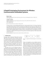
dependent stages for object detection. Most research on ob-
ject detection involves 4 stages: preprocessing, segmentation,
feature e xtraction,andclassification [13, 14, 15], as shown in
Figure 1. The preprocessing stage aims to remove noise or
enhance edges. In the segmentation stage, a number of co-
herent regions and “suspicious” regions which might con-
tain objects are usually located and separated from the entire
images. The feature extraction stage extracts domain-specific
features from the segmented regions. Finally, the classifica-
tion stage uses these features to distinguish the classes of
the objects of interest. The algorithms or methods for these
stages are generally domain specific. Learning paradigms,
such as NNs and genetic algorithms/programming, have
usually been applied to the classification stage. In general,
each independent stage needs a program to fulfill that spe-
cific task and, accordingly, multiple programs are needed for
object detection problems. Success at each stage is critical
Multiclass Object Detection Using Genetic Programming 843
Source
databases
Preprocessing Segmentation
Feature
extraction

Classification
(1) (2) (3) (4)
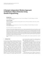
Figure 1: A typical procedure for object detection.
to achieving good final detection performance. Detection of
trucks and tanks in visible, multispectral infrared, and syn-
thetic aperture radar images [2], and recognition of tanks in
cluttered images [6] are two examples.
(ii) Single-stage approach, which uses only a single stage
to detect the objects of interest in large images. There is only a
single program produced for the whole object detection pro-
cedure. The major property of this approach is that it is seg-
mentation free. Detecting tanks in infrared images [3]and
detecting small targets in cluttered images [16]basedona
single NN are examples of this approach.
While most recent work on object detection problems
concentrates on the segmentation-based approach, this pa-
per focuses on the single-stage approach.
2.1.2 Domain-specific approach versus
domain-independent approach
In terms of the generalisation of the detection systems, there
are two major approaches.
(i) Domain-specific object detection, which uses specific
image features as inputs to the detector or classifier. These
features, which are usually highly domain dependent, are ex-
tracted from entire images or segmented images. In a lentil
grading and quality assessment system [17], for example, fea-
tures such as brigh tness, colour, size, and perimeter are ex-
tracted and used as inputs to an NN classifier. This approach
generally involves a time-consuming investigation of good
features for a specific problem and a handcrafting of the cor-

responding feature extraction programs.
(ii) Domain-independent object detection, which usually
uses the raw pixels directly (no features) as inputs to the
detector or classifier. In this case, feature selec tion, extrac-
tion, and the handcrafting of corresponding programs can
be completely removed. This approach usually needs learn-
ing and adaptive techniques to learn features for the detec-
tion task. Directly using raw image pixel data as input to
NNs for detecting vehicles (tanks, trucks, cars, etc.) in in-
frared images [1] is such an example. However, long learn-
ing/evolution times are usually required due to the large
number of pixels. Furthermore, the approach generally re-
quires a large number of training examples [18]. A special
case is to use a small number of domain-independent, pixel
level features (referred to as pixel statistics) such as the mean
and variance of some portions of an image [19].
2.1.3 Multiple class versus single class
Regarding the number of object classes of interest in an im-
age, there are two main types of detection problems.
(i) One-class object detection problem, where there are
multiple objec ts in each image, however they belong to a sin-
gle class. One special case in this category is that there is only
oneobjectofinterestineachsourceimage.Innature,these
problems contain a binary classification problem: object ver-
sus nonobject, also called object versus backg round. Examples
are detecting small targets in thermal infr ared images [16]
and detecting a particular face in photograph images [20].
(ii) Multiple-class object detection problem, where there
are multiple object classes of interest, each of which has mul-
tiple objects in each image. Detection of handwritten digits

in zip code images [21] is an example of this kind.
It is possible to view a multiclass problem as series of bi-
nary problems. A problem with objects 3 classes of interest
can be implemented as class1 against everything else, class2
against everything else, and class 3 against everything else.
However, these are not independent detectors as some meth-
ods of dealing with situations when two detectors repor t an
object at the same location must be provided.
In general, multiple-class object detection problems are
more difficult than one-class detection problems. This paper
is focused on detecting multiple objec ts from a number of
classes in a set of images, which is particularly difficult. Most
research in object detection which has been done so far be-
longs to the one-class object detection problem.
2.2. Performance evaluation
In this paper, we use the DR and FAR to measure the per-
formance of multiclass object detection problems. The DR
refers to the number of small objects correctly repor ted by a
detection system as a percentage of the total number of ac-
tual objects in the image(s). The FAR, also called false alarms
per object or false alarms/obj ect [16], refers to the number
of nonobjects incorrectly reported as objects by a detection
system as a percentage of the total number of actual objects
in the image(s). Note that the DR is between 0 and 100%,
while the FAR may be greater than 100% for difficult object
detection problems.
The main goal of objec t detection is to obtain a high DR
and a low FAR. There is, however, a trade-off between them
for a detection system. Trying to improve the DR often results
in an increase in the FAR, and vice versa. Detecting objects in

images with very cluttered backgrounds is an extremely dif-
ficult problem where FARs of 200–2000% (i.e., the detection
system suggests that there are 20 times as many objects as
there really are) are common [5, 16].
Most research which has been done in this area so far only
presents the results of the classification stage (only the final
stage in Figure 1) and assumes that all other stages have been
properly done. However, the results presented in this paper
are the performance for the whole detection problem (both
the localisation and the classification).
844 EURASIP Journal on Applied Signal Processing
2.3. Related work—GP for object detection
Since the early 1990s, there has been only a small amount
of work on applying GP techniques to object classification,
object detection, and other vision problems. This, in part,
reflects the fact that GP is a relatively young discipline com-
pared with, say, NNs.
2.3.1 Object classification
Tackett [9, 22] uses GP to assign detected image features to a
target or nontarget category. Seven primitive image features
and twenty statistical features are extracted and used as the
terminal set. The 4 standard arithmetic operators and a logic
function are used as the function set. The fitness function is
based on the classification result. The approach was tested
on US Army NVEOD Terrain Board imagery, where vehicles,
such as tanks, need to be classified. The GP method outper-
formed both an NN classifier and a binar y tree classifier on
the same data, producing lower rates of false positives for the
same DRs.
Andre [ 23 ] uses GP to evolve f unctions that traverse an

image, calling upon coevolved detectors in the form of hit-
miss matrices to guide the search. These hit-miss matrices
are evolved with a two-dimensional genetic algorithm. These
evolved functions are used to discriminate between two let-
ters or to recognise single digits.
Koza in [24, Chapter 15] uses a “turtle” to walk over a
bitmap landscape. This bitmap is to be classified either as a
letter “L,” a letter “I,” or neither of them. The turtle has ac-
cess to the values of the pixels in the bitmap by moving over
them and calling a detector primitive. The turtle uses a deci-
sion tree process, in conjunction with negative primitives, to
walk over the bitmap and decide which category a particular
landscape falls into. Using automatically defined functions as
local detectors and a constrained syntactic structure, some
perfect scoring classification programs were found. Further
experiments showed that detectors can be made for different
sizes and positions of letters, although each detector has to
be specialised to a given combination of these factors.
Te l ler an d Ve lo s o [11] use a GP method based on the
PADO language to perform face recognition tasks on a
database of face images in which the evolved programs have
a local indexed memory. The approach was tested on a
discrimination task between 5 classes of images [25]and
achieved up to 60% correct classification for images without
noise.
Robinson and McIlroy [26] apply GP techniques to the
problem of eye location in grey-level face images. The in-
put data from the images is restricted to a 3000-pixel block
around the location of the eyes in the face image. This ap-
proach produced promising results over a very small train-

ing set, up to 100% tr ue positive detection with no false pos-
itives, on a three-image training set. Over larger sets, the GP
approach performed less well however, and could not match
the performance of NN techniques.
Winkeler and Manjunath [10] produce genetic programs
to locate faces in images. Face samples are cut out and
scaled, then preprocessed for feature extraction. The statis-
tics gleaned from these segments are used as terminals in GP
which evolves an expression returning how likely a pixel is
to be part of a face image. Separate experiments process the
grey-scale image directly, using low-level image processing
primitives and scale-space filters.
2.3.2 Object detec tion
All of the reported GP-based object detection approaches be-
long to the one-class object detection category. In these detec-
tion problems, there is only one object class of interest in the
large images.
Howard et al. [19] present a GP approach to automatic
detection of ships in low-resolution synthetic aperture radar
imagery. A number of random integer/real constants and
pixel statistics are used as terminals. The 4 arithmetic op-
erators and min and max operators constitute the function
set. The fitness is based on the number of the true positive
and false positive objects detected by the evolved program.
A two-stage evolution strategy was used in this approach. In
the first stage, GP evolved a detector that could correctly dis-
tinguish the target (ship) pixels from the nontarget (ocean)
pixels. The best detector was then applied to the entire im-
age and produced a number of false alarms. In the second
stage, a brand new run of GP was tasked to discriminate be-

tween the clear targets and the false alarms as identified in the
first stage and another detector was generated. This two-stage
process resulted in two detectors that were then fused using
the min function. These two detectors return a real number,
which if greater than zero denotes a ship pixel, and if zero or
less denotes an ocean pixel. The approach was tested on im-
ages chosen from commercial SAR imagery, a set of 50 m and
100 m resolution images of the English Channel taken by the
European Remote Sensing satellite. One of the 100 m resolu-
tion images was used for training, two for validation, and two
for testing. The training was quite successful with perfec t DR
and no false alarms, while there was only one false positive
in each of the two test images and the two validation images
which contained 22, 22, 48, and 41 t rue objects.
Isaka [27] uses GP to locate mouth corners in small
(50 × 40) images taken from images of faces. Processing each
pixel independently using an approach based on relative in-
tensities of surrounding pixels, the GP approach was shown
to perform comparably to a template matching approach on
the same data.
A list of object detection related work based on GP is
shown in Ta b l e 1 .
3. GP ADAPTED TO MULTICL ASS OBJECT DETECTION
3.1. The GP system
Inthissection,wedescribeourapproachtoaGPsystemfor
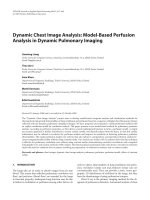
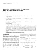
multiple-class object detection problems. Figure 2 shows an
overview of this approach, which has a learning process and
a testing procedure. In the learning/e volutionary process, the
evolved genetic programs use a square input field which is
large enough to contain each of the objects of interest. The

programs are applied in a m oving window fashion to the
Multiclass Object Detection Using Genetic Programming 845
Table 1: Object detection-related work based on GP.
Problems Applications Authors Year Source
Object classification
Tank detection
(classification)
Tackett 1993 [9]
Tackett 1994 [22]
Letter recognition
Andre 1994 [23]
Koza 1994 [24]
Face recognition Teller and Veloso 1995 [11]
Small target classification
Stanhope and Daida 1998 [28]
Winkeler and Manjunath 1997 [10]
Shape recognition Teller and Veloso 1995 [25]
Eye recognition Robinson and McIlroy 1995 [26]
Object detection
Ship detection Howard et al. 1999 [19]
Mouth detection Isaka 1997 [27]
Small target detection Benson 2000 [29]
Vehicle detection Howard et al. 2002 [30]
Other vision problems
Edge detection Lucier et al. 1998 [31]
San Mateo trail problem
Koza 1992 [32]
Koza 1993 [33]
Image analysis
Howard et al. 2001 [34]

Poli 1996 [35]
Model interpretation Lindblad et al. 2002 [36]
Stereoscopic vision Graae et al. 2000 [37]
Image compression Nordin and Banzhaf 1996 [38]
entire images in the training set to detect the objects of inter-
est. In the test procedure, the best evolved genetic program
obtained in the learning process is then applied to the en-
tire images in the test set to measure objec t detection perfor-
mance.
The learning/evolutionary process in our GP approach is
summarised as follows.
(1) Initialise the population.
(2) Repeat until a termination criterion is satisfied.
(2.1) Evaluate the individual programs in the current
population. Assign a fitness to each program.
(2.2) Until the new population is fully created, repeat
the following:
(i) select programs in the current generat ion;
(ii) perform genetic operators on the selected
programs;
(iii) insert the result of the genetic operations
into the new generation.
(3) Present the best individual in the population as the
output—the learned/evolved genetic program.
In this system, we used a tree-like program structure
to represent genetic programs. The ramped half-and-half
method was used for generating the programs in the initial
population and for the mutation operator. The proportional
selection mechanism and the reproduction, crossover, and
mutation operators were used in the learning process.

In the remainder of this section, we address the other as-
pects of the learning/evolutionary system: (1) determination
of the terminal set, (2) determination of the function set, (3)
development of a classification strategy, (4) construction of
the fitness measure, and (5) selection of the input parame-
ters and determination of the termination str ategy.
3.2. The terminal sets
For object detection problems, terminals generally corre-
spond to image features. In our approach, we designed three
different terminal sets: local rectilinear features, circular fea-
tures, and “pixel features.” In all these cases, the features are
statistical properties of regions of the image, and we refer to
them as pixel statistics.
3.2.1 Terminal set I—rectilinear features
In the first terminal set, twenty pixel statistics, F
1
to F
20
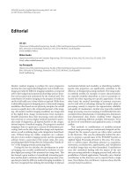
in Table 2, are extracted from the input field as shown in
Figure 3. The input field must be sufficiently large to contain
the biggest object and some background, yet small enough to
include only a single object. In this way, the evolved program,
as a detector, could automate the “human eye system” of
identifying pixels/object centres which stand out from their
local surroundings.
In Figure 3, the grey-filled circle denotes an object of in-
terest and the square A
1
B
1

C
1
D
1
represents the input field.
846 EURASIP Journal on Applied Signal Processing
Detection results
Object detection (GP testing)
General programs
Entire images
(detection test set)
GP learning/evolutionary process
Entire images
(detection training set)
Figure 2: An overview of the GP approach for multiple-class object
detection.
Table 2: Twenty pixel statistics. (SD: standard deviation.)
Pixel statistics
Regions and lines of interest
Mean SD
F
1
F
2
big square A
1
B
1
C
1

D
1
F
3
F
4
small central square A
2
B
2
C
2
D
2
F
5
F
6
upper left square A
1
E
1
OG
1
F
7
F
8
upper right square E
1

B
1
H
1
O
F
9
F
10
lower left square G
1
OF
1
D
1
F
11
F
12
lower right square OH
1
C
1
F
1
F
13
F
14
central row of the big square G

1
H
1
F
15
F
16
central column of the big square E
1
F
1
F
17
F
18
central row of the small square G
2
H
2
F
19
F
20
central column of the small square E
2
F
2
The five smaller squares represent local regions from which
pixel statistics will b e computed. The 4 central lines (rows
and columns) are also used for a similar purpose.

1
The mean
and standard deviation of the pixels comprising each of these
regions are used as two separate features. There are 6 regions
giving 12 features, F
1
to F
12
. We also use pixels along the main
axes (4 lines) of the input field, giving features F
13
to F
20
.
In addition to these pixel statistics, we use a terminal
which generates a random constant in the range [0, 255].
This corresponds to the range of pixel intensities in grey-level
images.
These pixel statistics have the following characteristics.
(i) They are symmetrical.
1
These lines can be considered special local regions. If the input field size
n is an even number, each of these “lines” is a rectangle consisting of two
rows or two columns of pixels.
(ii) Local regional features (from small squares and lines)
are included. This assists the finding of object centres
in the sweeping procedure—if the evolved program is
considered as a moving window template, the match
between the template and the subimage forming the
input field will be better when the moving template is

close to the centre of an object.
(iii) They are domain-independent and easy to extract.
These features belong to the pixel level and can be part
of a domain-independent preexisting feature library of
terminals from which the GP evolutionary process is
expected to automatically learn and select only those
relevant to a particular domain. This is quite different
from the traditional image processing and computer
vision approaches where the problem-specific features
are often needed.
(iv) The number of these features is fixed. In this approach,
the number of features is always twenty no matter what
size the input field is. This is particularly useful for the
generalisation of the system implementation.
3.2.2 Terminal set II—circular features
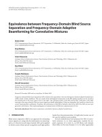
The second terminal set is based on a number of circular
features, as shown in Figure 4.Thefeatureswerecomputed
based on a series of concentric circles centred in the input
field. This terminal set focused on boundaries rather than re-
gions. The gap between the radii of two neighbouring circles
is one pixel. For instance, if the input field is 19 × 19 pix-
els, then the number of central circles wil l be 19/2+1= 10
(the central pixel is considered as a circle with a zero radius);
accordingly, there would be 20 features. Compared with the
rectilinear terminal set, the number of these circular fea-
tures in this terminal set depends on the size of the input
field.
3.2.3 Terminal set III—pixels
The goal of this terminal set is to investigate the use of raw
pixels as terminals in GP. To decrease the computation cost,

we considered a 2 × 2 square, or 4 pixels, as a single pixel.
The average value of the 4 pixels in the square was used as
the value of this pixel, as shown in Figure 5.
3.3. The function sets
We used two different function sets in the exper iments: 4
arithmetic operations only, and a combination of arithmetic
and transcendental functions.
3.3.1 Function set I
In the first function set, the 4 standard arithmetic operations
were used to form the nonterminal nodes:
FuncSet1
={+, −, ∗,/}. (1)
The +, −,and∗ operators have their usual meanings—
addition, subtraction, and multiplication, while / represents
“protected” division which is the usual division operator
Multiclass Object Detection Using Genetic Programming 847
n
n
n/2 n/2
n/2 n/2
D
1
F
1
C
1
D
2
F
2

C
2
G
1
G
2
O
H
2
H
1
A
2
E
2
B
2
A
1
E
1
B
1
Squares:
A
1
B
1
C
1

D
1
, A
2
B
2
C
2
D
2
,
A
1
E
1
OG
1
, E
1
B
1
H
1
O,
G
1
OF
1
D
1

, OH
1
C
1
F
1
Rows and columns (lines):
G
1
H
1
, E
1
F
1
, G
2
H
2
, E
2
F
2
Size of the lines:
G
2
H
2
= A
2

B
2
= E
2
F
2
= B
2
C
2
:
User defined; Default = n/2
Figure 3: The input field and the image regions and lines for feature selection in constructing terminals.
O
C
1
C
2
··· C
i
···C
n
Features
Local boundaries
Mean SD
F
1
F
2
Central pixel

F
3
F
4
Circular boundary C
1
F
5
F
6
Circular boundary C
2
.
.
.
.
.
.
.
.
.
F
(2i+1)
F
(2i+2)
Circular boundary C
i
.
.
.

.
.
.
.
.
.
F
(2n+1)
F
(2n+2)
Circular boundary C
n
Figure 4: The input field and the image boundaries for feature extra ction in constructing terminals.
Figure 5: Pixel terminals.
except that a divide by zero gives a result of zero. Each of
these functions takes two arguments. This function set was
designed to investigate whether the 4 standard arithmetic
functions are sufficient for the multiple-class object detec-
tion problems.
A generated program consisting of the 4 functions and
a number of rectilinear terminals is shown in Figure 6.The
LISP form of this program is shown in Figure 7.
This program performed particularly well for the coin
images.
3.3.2 Function set II
We also designed a second function set. We hypothesized
that convergence might be quicker if the function values were
close to the range (
−1, 1) and more functions might lead to
better results if the 4 ar ithmetic functions were not sufficient.

We introduced some transcendental functions, that is, the
absolute function dabs, the trigonometric sine function sin,
the logarithmetic function log, and the exponent (to base e)
function exp, to form the second function set:
FuncSet2
={+, −, ∗,/,dabs, sin, log, exp}. (2)
3.4. Object classification strategy
The output of a genetic program in a standard GP sys-
tem is a floating point number. Genetic programs can be
848 EURASIP Journal on Applied Signal Processing
F
16
F
14
+ F
5
+
F
11
F
14
· F
20
F
11
+ F
12
− F
14
− (F

9
· F
11
· F
1
· F
10
− F
9
· F
17
) ·
F
5
F
18
−

F
17
+(F
11
+ F
12
) · F
20
+

F
2

+ 145.765 −
F
6
F
11

· (133.082 − F
17
) ·
F
11
F
14
· F
20

+

(F
6
− F
5
− F
3
· F
6
) ·
F
1
+ 145.765 + F

16
· F
10
F
18
− F
12

· [F
17
+(F
17
+ F
12
) · F
20
+ F
14
· F
12
· (F
1
+ F
12
− F
17
)]
Figure 6: A generated program for the coin detection problem.
(+ (- (+ (+ (/ F
16

F
14
) F
5
)(+(/(/F
11
(* F
14
F
20
)) F
11
)(-F
12
F
14
))) (- (* (- (* (* (* F
9
F
11
) F
1
) F
10
)(*F
9
F
17
)) (/ F
5

F
18
)) (-
(+ (+ F
17
(* (+ F
11
F
12
) F
20
)) (* (- (+ F
2
145.765) (/ F
6
F
11
)) (-
133.082 F
17
))) (/ F
11
(* F
14
F
20
))))) (* (- (* (- (- F
6
F
5

)(*F
3
F
6
)) (/ (+ (+ F
1
145.765) (* F
16
F
10
)) F
18
)) F
12
)(+(+F
17
(* (+ F
17
F
12
) F
20
)) (* (+ F
14
F
12
)(-(+F
1
F
12

) F
17
)))))
Figure 7: LISP format of the generated program in Figure 6.
used to perform one-class object detection tasks by utilis-
ing the division between negative and nonnegative num-
bers of a genetic program output. For example, negative
numbers can correspond to the background and nonneg-
ative numbers to the objects in the (single) class of inter-
est. This is similar to binary classification problems in stan-
dard GP where the division between negative and nonneg-
ative numbers acts as a natural boundary for a distinction
between the two classes. Thus, genetic programs generated
by the standard GP evolutionary process primarily have the
ability to represent and process binary classification or one-
class object detection tasks. However, for the multiple-class
object detection problems described here, where more than
two classes of objects of interest are involved, the standard
GP classification strategy mentioned above cannot be ap-
plied.
In this approach, we develop a different strategy which
uses a program classification map, as shown in Figure 8,for
the multiple-class object detection problems. Based on the
output of an evolved genetic program, this map can identify
which class of the object located in the current input field be-
longs to. In this map, m refers to the number of object classes
of interest, v is the output value of the evolved program, and
T is a constant defined by the user, which plays a role of a
threshold.
3.5. The fitness function

Since the goal of object detection is to achieve both a high DR
and a low FAR, we should consider a multiobjective fitness
function in our GP system for multiple-class object detection
problems. In this approach, the fitness function is based on
a combination of the DR and the FAR on the images in the
training set during the learning process. Figure 9 shows the
object detection procedure and how the fitness of an evolved
genetic program is obtained.
The fitness of a genetic program is obtained as follows.
(1) Apply the program as a moving n×n window template
(n is the size of the input field) to each of the training
images and obtain the output value of the program at
each possible window position. Label each window po-
sition with the “detected” object according to the ob-
ject classification strategy described in Figure 8.Call
this data structure a detection map. An object in a de-
tection map is associated with a floating point pro-
gram output.
(2) Find the centres of objects of interest only.Thisisdone
as follows. Scan the detection map for an object of in-
terest. When one is found, mark this point as the centre
of the object and continue the scan n/2 pixels later in
both horizontal and vertical directions.
(3) Match these detected objects with the known locations
of each of the desired true objects and their classes. A
match is considered to occur if the detected object is
within tolerance pixels of its known true location. A
tolerance of 2 means that an object whose true loca-
tion is (40, 40) would be counted as correctly located
at (42, 38) but not at (43, 38). The tolerance is a con-

stant parameter defined by the user.
(4) Calculate the DR and the FAR of the evolved program.
(5) Compute the fitness of the program as follows:
fitness(FAR, DR)
= W
f
× FAR + W
d
× (1 − DR), (3)
Multiclass Object Detection Using Genetic Programming 849
Class =




































background,v<0,
class 1, 0 ≤ v ≤ T,
class 2,T≤ v ≤ 2T,
.
.
.
.
.
.
class i, (i − 1) × T ≤ v ≤ i × T,
.
.
.
.

.
.
class m, v ≥ i × T,
Background
Class 1
.
.
.
Class i
.
.
.
Class m
0
T
···
i × T
···
(m− 1)× T
v
Figure 8: Mapping of program output to an object classification.
Compute fitness
Calculate DR and FAR
Match objects
Find object centre
Sweep programs
on training images
Figure 9: Object detection and fitness calculation.
where W
f

and W
d
are constant weights which reflect
the relative importance of FAR versus DR.
2
With this design, the smaller the fitness, the better the
performance. Zero fitness is the ideal case, which corre-
sponds to the situation in which all of the objects of inter-
est in each class are correctly found by the evolved program
without any false alarms.
3.6. Main parameters
Once a GP system has been created, one must choose a set
of parameters for a run. Based on the roles they play in the
learning/evolutionar y process, we group these parameters
2
Theoretically, W
f
and W
d
could be replaced by a single parameter since
they have only one degree of freedom. However, the two cases of using a sin-
gle and double parameters have different effects for stopping the evolution-
ary process. For convenience, we use two parameters.
into three categories: search parameters, genetic parameters,
and fitness parameters.
3.6.1 Search parameters
The search parameters used here include the number of in-
dividuals in the population (population-size), the maximum
depth of the ra ndomly generated programs in the initial pop-
ulation (initial-max-depth), the maximum depth permitted

for programs resulting from crossover and mutation opera-
tions (max-depth), and the maximum generations the evo-
lutionary process can run (max-generations). These parame-
ters control the search space and when to stop the learning
process. In theory, the larger these parameters, the more the
chance of success. In practice, however, it is impossible to set
them very large due to the limitations of the hardware and
high cost of computation.
There is another search parameter, the size of the input
field (input-size), which decides the size of the moving win-
dow in which a genetic program is computed in the program
sweeping procedure.
3.6.2 Genetic parameters
The genetic parameters decide the number of genetic pro-
grams used/produced by different genetic operators in the
mating pool to produce new programs in the next gener-
ation. These parameters include the percentage of the best
individuals in the cur rent population that are copied un-
changed to the next generation (reproduction-rate), the per-
centage of individuals in the next generation that are to be
produced by crossover (cross-rate), the percentage of individ-
uals in the next generation that are to be produced by muta-
tion (mutati on-rate
= 100%−reproduction-rate−cross-rate),
the probability that, in a crossover operation, two termi-
nals will be swapped (cross-term), and the probability that,
in a crossover operation, random subtrees will be swapped
(cross-func = 100% − cross-term).
3.6.3 Fitness parameters
The fitness parameters include a threshold parameter (T)

in the object classification algorithm, a tolerance parameter
850 EURASIP Journal on Applied Signal Processing
Table 3: Parameters used for GP training for the three databases.
Parameter kinds Parameter names Easy images Coin images Retina images
Search parameters
Population-size 100 500 700
Initial-max-depth 4 5 6
Max-depth 8 12 20
Max-generations 100 150 150
Input-size 14 × 14 24 × 24 16 × 16
Genetic parameters
Reproduction-rate 10% 1% 2%
Cross-rate 65% 74% 73%
Mutation-rate 25% 25% 25%
Cross-term 15% 15% 15%
Cross-func 85% 85% 85%
Fitness parameters
T 100 100 100
W
f
50 50 50
W
d
1000 1000 3000
Tolerance (pixels) 2 2 2
(tolerance) in object matching, and two constant weight
parameters (W
f
and W
d

) reflecting the relative importance
of the DR and the FAR in obtaining the fitness of a genetic
program.
3.6.4 Parameter values
Good selection of these parameters is crucial to success. The
parameter values can be very different for various object de-
tection tasks. However, there does not seem to be a reliable
way of apriorideciding these parameter values. To obtain
good results, these parameter values were carefully chosen
through an empirical search in experiments. Values used are
shown in Ta b le 3 .
For detecting circles and squares in the easy images, for
example, we set the population size to 100. On each itera-
tion, 10 programs are created by reproduction, 65 programs
by crossover, and 25 by mutation. Of the 65 crossover pro-
grams, 10 (15%) are generated by swapping terminals and
55 (85%) by swapping subtrees. The programs are randomly
initialised with a maximum depth of 4 at the beginning and
the depth can be increased to 8 during the evolutionary pro-
cess. We also use 100, 50, 1000, and 2 as the constant pa-
rameters T, W
f
, W
d
,andtolerance, which are used for the
program classification and the calculation of the fitness func-
tion. The maximum generation permitted for the evolution-
ary process is 100 for this detection problem. The size of the
input field is the same as that used in the NN approach [12],
that is, 14 × 14.

3.7. Termination criteria
In this approach, the learning/evolutionary process is termi-
nated when one of the following conditions is met.
(i) The detection problem has been solved on the training
set, that is, all objects in each class of interest in the
training set have been correctly detected with no false
alarms. In this case, the fitness of the best individual
program is zero.
(ii) The number of generations reaches the predefined
number, max-generations. Max-generations was deter-
mined empirically in a number of preliminary runs as
a point before overtraining generally occurred. While
it would have been possible to use a validation set to
determine when to stop training, we have not done
this. Comparison of training and test DRs and FARs
indicated that overfitting was not significant.
4. THE IMAGE DATABASES
We used three different databases in the experiments. Exam-
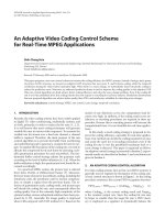
ple images and key characteristics are given in Figure 10.The
databases were selected to provide detection problems of in-
creasing difficult y. Database 1 (easy) was generated to give
well-defined objects against a uniform background. The pix-
els of the objects were generated using a Gaussian genera-
tor with different means and variances for each class. There
are three classes of small objects of interest in this database:
black circles (class1), grey squares (class2), and white circles
(class3). The Australian coin images (database 2) were in-
tended to be somewhat harder and were taken with a CCD
camera over a number of days with relatively similar illumi-
nation. In these images, the background varies slightly in dif-

ferent areas of the image and between images, and the objects
to be detected are more complex, but still regular. There are
4 objec t classes of interest: the head side of 5-cent coins (class
head005), the head side of 20-cent coins (class head020), the
tail side of 5-cent coins (class tail005), and the tail side of 20-
cent coins (class tail020). All the objects in each class have
a similar size. They are located at arbitrary positions and
with some rotations. The retina images (database 3) were
taken by a professional photographer with special appara-
tus at a clinic and contain very irregular objects on a very
Multiclass Object Detection Using Genetic Programming 851
Number of images: 10
Object classes: 3
Image size 700 × 700
(a) Easy (circles and squares).
Number of images: 20
Object classes: 4
Image size 640 × 680
(b) Medium difficulty (coins).
Number of images: 15
Object classes: 2
Image size 1024 × 1024
(c) Very difficult (retinas).
Figure 10: Object detection problems of increasing difficulty.
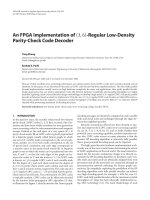
Figure 11: An enlarged view of one piece of the retina images.
cluttered background. The objective is to find two classes of
retinal pathologies—haemorrhages and microaneurisms. To
give a clear view of representative samples of the target ob-
jects in the retina images, one sample piece of these images is
presented in Figure 11. In this figure, haemorrh age and mi-

croaneurism examples are labeled using white surrounding
squares.
5. EXPERIMENTAL RESULTS
We performed three groups of experiments, as shown in
Table 4. The first group of experiments is based on the first
two terminal sets (rectilinear features and circular features)
and the first function set (the 4 standard arithmetic func-
tions). The second group of experiments uses the third ter-
minal set consisting of raw “pixel” and the first function set.
The third group of experiments uses the first terminal set
consisting of rectilinear features and the second function set
consisting of additional transcendental functions.
Table 4: Three groups of experiments.
Experiments Terminal sets Function sets
I
TermSet1 (rectilinear) FuncSet1
TermSet2 (circular) FuncSet1
II TermSet3 (pixels) FuncSet1
III TermSet1 (rectilinear) FuncSet2
In these experiments, 4 out of 10 images in the easy im-
age database are used for training and 6 for testing. For the
coin images, 10 out of 20 are used for training and 10 for
testing. For the retina images, 10 are used for training and
5 for testing. The total number of objects is 300 for the easy
image database, 400 for the Australian coin images, and 328
for the retina images. The results presented in this section
were achieved by applying the evolved genetic programs to
the images in the test sets.
5.1. Experiment I
This group constitutes the major part of the investiga-

tion. T he main goal here is to investigate whether this
GP approach can be applied to multiple-class object detec-
tion problems of increasing difficulty. The parameters used
in these exper iments are shown in Table 3 (Section 3.6.4).
The average performance of the best 10 genetic programs
(evolved from 10 runs) for the easy and the coin databases,
and the average performance of the best 5 genetic programs
(out of 5 runs, due to the high computational cost) for the
retina images are presented.
The results are compared with those obtained using an
NN approach for object detection on the same databases
852 EURASIP Journal on Applied Signal Processing
[12, 39]. The NN method used was the same as the GP
method shown in Section 1.1, except that the evolutionary
process was replaced by a network training process in step
(3) and the generated genetic program was replaced by a
trained network. In this group of experiments, the networks
also used the same set of pixel statistics as TermSet1 (recti-
linear) as inputs. Considerable effort was expended in deter-
mining the best network architectures and training parame-
ters. The results presented here are the best results achieved
by the NNs and we believe that the comparison with the GP
approach is a fair one.
5.1.1 Easy images
Table 5 shows the best results of the GP approach with the
two different terminal sets (GP1 with TermSet1, GP2 with
TermSet2) and the NN method for the easy images. For class1
(black circles) and class3 (grey circles), all the three methods
achieved a 100% DR with no false alarms. For class2 (grey
squares), the two GP methods also achieved 100% DR with

zero false alarms. However, the NN method had an FAR of
91.2% at a DR of 100%.
5.1.2 Coin images
Experiments with coin images gave similar results to the easy
images. These are shown in Table 6. Detecting the heads and
tails of 5 cents (class head005, tail005)appearstoberelatively
straig ht forward. All the three methods achieved a 100% DR
without any false alarms. Detecting heads and tails of 20-
cent coins (class head020, tail020)ismoredifficult. While the
NN method resulted in many false alarms, the two GP meth-
ods had much better results. In particular, the GP1 method
achieved the ideal results, that is, all the objec ts of interest
were correctly detected without any false alarms for all the 4
object classes.
5.1.3 Retina images
The results for the retina images are summarised in Table 7.
Compared with the results for the other image databases,
these results are not satisfactory.
3
However, the FAR is greatly
improved over the NN method.
The results over the three databases show similar pat-
terns: the GP-based method always gave a lower FAR than
the NN approach for the same detection rate. While GP2 also
gave the ideal results for the easy images, it produced a higher
FAR on both the coin and the retina images than the GP1
method. This suggests that the local rectilinear features are
more effective for these detection problems than the circular
features.
5.1.4 Training times

We performed these experiments on a 4-processor ULTRA-
SPARC4. The t raining times for the three databases are very
3
With the current techniques applied in this area, detecting objects in
images with a highly cluttered background is an extremely difficult problem
[5, 16]. In fact, these results are quite competitive to other methods for very
difficult detection problems. As a young discipline, it is quite promising for
GP to achieve such results.
Table 5: Comparison of the object detection results for the easy
images: the GP approaches versus the NN approach. (Input field
size = 14 × 14; repetitions = 10.)
Easy images
Object classes
class1 class2 class3
Best detection rate (%) 100 100 100
False alarm rate (%)
NN 0 91.2 0
GP1 0 0 0
GP2 0 0 0
Table 6: Comparison of the object detection results for the coin
images. The GP approaches versus the NN approach. (Input field
size = 24 × 24, repetitions = 10.)
Coin images
Object classes
head005 tail005 head020 tail020
Best detection rate (%) 100 100 100 100
False alarm rate (%)
NN 0 0 182 37.5
GP10000
GP2 0 0 38.4 26.7

Table 7: Comparison of the object detection results for the retina
images. The GP approaches versus the NN approach. (Input field
size = 16 × 16, repetitions = 5.)
Retina images
Object classes
Haem Micro
Best detection rate (%) 73.91 100
False alarm rate
(%)
NN 2859 10104
GP1 1357 588
GP2 1857 732
different due to various degrees of difficulty of the detec-
tion problems. The average training times used in the GP
evolutionary process (GP1) for the easy, the coin, and the
retina images are 2 minutes, 36 hours, and 93 hours, respec-
tively.
4
This is much longer than the NN method, which took
2 minutes, 35 minutes, and 2 hours on average. However,
the GP method gave much better detection results on all the
three databases. This suggests that the GP method is partic-
ularly applicable to tasks where accuracy is the most impor-
tant factor and training time is seen as relatively unimpor-
tant.
4
Even if the training time for difficult problems is very long, the time
spent on applying the learned genetic program to the test set is usually very
short, say, from several seconds to about one minute.
Multiclass Object Detection Using Genetic Programming 853

Table 8: Results with the second function set.
Easy images Coin images Retina images
Class1 Class2 Class3 Head005 Tail005 Head020 Tail020 Haem Micro
Best detection rate (%) 100 100 100 100 100 100 100 73.91 100
Falsealarmrate(%)00000001214 463
5.2. Experiment II
Instead of using rectilinear and circular features (pixel statis-
tics) as in experiment I, experiment II directly uses the pixel
values as terminals (the third terminal set). For the input
field sizes of 14 × 14, 24 × 24, and 16 × 16, for the easy, the
coin, and the retina images, the number of terminals are 49
(7×7), 144 (12×12), a nd 64 (8×8), respectively. For the easy
images, the learning took about 70 hours on a 4-processor
ULTRA-SPARC4 machine to reach perfect detection perfor-
mance on the training set and 78 generations were taken. The
population size used was 1000, the maximum depth of the
program was 30, the maximum initial depth 10, the max-
imum number of generations 100. For the coin images and
the retina images, the situation was worse. Since a large num-
ber of terminals were used, the maximum depth of the pro-
gram trees was increased to 50 for the coin images and 60
for the retina images. The population size for both databases
used was 3000 with a maximum number of generations of
100. The evolutionar y process took three weeks to complete
50 generations for the coin images and five weeks to complete
50 generations for the retina images. The best detection re-
sults were overall 22% FAR at a 100% DR for the coin images,
and about 850% FAR at a DR of 100% for microaneurisms
in the retina images.
While these results are worse than those obtained by the

GP1 and GP2 using the rectilinear and circular features, they
are still better than the NN approach. If we use a larger popu-
lation (e.g., 10000 or 50000), a larger program size (e.g., 100),
and a larger number of generations (e.g., 300), the results
could be better according to our experience. While this is not
possible to investigate with the current hardware we use, it
shows a promising future direction with the improvement
and development of more powerful hardware, for example,
parallel or genetic hardware.
5.3. Experiment III
Instead of using the four standard arithmetic functions,
this experiment focused on using the extended function
set (FuncSet2), as shown in Section 3.3.2.Theparameters
shown in Table 3 (Section 3.6.4) were used in this experi-
ment. The best detection results for the three databases are
shown in Ta b le 8 .
AscanbeseenfromTable 8, this function set also gave
ideal results for the easy and the coin images and a better
result for the retina images. The best DR for detecting micro
is 100% with a corresponding FAR of 463%. The best DR
for haem is still 73.91% but the FAR is reduced to 1214%. In
addition, convergence was slightly faster for training the coin
and retina images. T his suggests that dabs, sin, log, and exp
are particularly useful for more difficult problems.
6. DISCUSSION
6.1. Analysis of results on the retina images
The GP-based approach achieved the ideal results on the easy
images and the coin images, but resulted in some false alar ms
on the retina images, particularly for the detection of objects
in class haem in which the FAR was very high and more than

a quarter of the real objects in this class were not detected by
the evolved genetic program.
We identified two possible reasons for the results on the
retina images being worse than the results on the easy and the
coin images. The first reason concerns the complexity of the
background. In the easy and coin images, the background is
relatively uniform, whereas in the retina images it is highly
cluttered. In particular, the background of the retina images
contains many objects, such as veins and other anatomical
features, that are not members of the two classes of inter-
est (microaneurisms and haemorrhages). These objects of
noninterest must be classified as “background,” in just the
same way as the genuine background. The more complex the
boundary between classes in the input space, the more com-
plex an evolved program has to be to distinguish the classes.
It may be that the more complex background class in the
retina images requires a more complex evolved program than
the GP system was able to discover. It may even be that the
set of terminals and functions is not adequate/sufficient to
represent an evolved program to distinguish the objects of
interest from such a rich background.
The second possible reason concerns the variation in size
of the objects. In the easy and coin images, all of the ob-
jects in a class have similar sizes, whereas in the retina im-
ages, the sizes of the objects in each class vary. This variation
means that the evolved genetic program must cover a more
complicated region of the input space. The sizes of the mi-
cro objects vary from 3
× 3to5× 5 pixels and the sizes of
the haem objects vary from 6 × 6to14× 14 pixels. Given

the size of the input field (16 × 16) and the choice of termi-
nals, the variance in the size of the haem objectsispartic-
ularlyproblematicsinceitrangesfromjustonequarterof
the input field ( hence entirely inside the central detection re-
gion) to almost the entire input field. The fact that the per-
formance on the haem class is worse than the performance
on the micro class (especially in experiment III) provides
854 EURASIP Journal on Applied Signal Processing
Program 1
F
3
· F
14
· F
15
F
6
· F
14
− F
19
− F
7
· F
10
· F
17
· F
16
· F

18
+
F
5
F
5
· F
14
+
F
3
F
5
F
3
F
5
·
F
5
F
6
F
11
F
15
+
F
19
F

6
F
5
F
15
Program 2
F
18
F
3
+ F
5
− F
3
· F
5
− F
4
· F
16
·
F
18
· (F
5
+ F
18
) − (F
7
+ F

4
)+F
10
− F
19
F
4
· F
16
Program 3
(F
16
+ F
7
) · F
15
· F
4
F
19
−
F
13
· F
5
F
18
F
10
+ F

11
·
F
9
F
9
· F
4
Figure 12: Three sample generated programs for simple object detection in the easy images.
(/ (+ (- (- (/ (* (* F
3
F
14
) F
15
) (* F
6
F
14
)) F
19
)(*(*(*(*F
7
F
10
) F
17
)
F
16

) F
18
)) (+ (* (/ F
5
F
5
) F
14
)(/F
3
F
5
))) (+ (* (/ F
3
F
5
)(/(/F
5
F
6
)(/
F
11
F
15
))) (/ (/ F
19
F
6
)(/F

5
F
15
))))
Figure 13: LISP format of Program 1.
additional evidence that the size variation is a cause of the
poor performance.
The first reason suggests that the current approach is lim-
ited on images containing cluttered backgrounds. One pos-
sible modification to address this limitation is to evolve mul-
tiple programs rather than a single program, either having
a separate program for each class of interest, or having sev-
eral programs to exclude different parts of the background.
Another possible modification is to extend the terminal set
and/or function set to enrich the expressive power of the
evolved programs.
The second reason suggests that the current approach has
limited applicability to scale invariant detection problems.
This would not be surprising, given the current set of termi-
nals and functions. In particular, although the pixel statistics
used in the rectilinear and circular terminal sets are robust
to small variations in scale, they are not robust to large varia-
tions. We will explore alternative pixel statistics that are more
robust to scale variations, and also function sets that would
allow disjunctive programs that could better represent classes
that contained objects of several different size ranges.
6.2. Analysis of evolved programs
This section gives a brief analysis of the best generated pro-
grams for the three databases. The genetic programs evolved
by the GP1 in experiment I are used as examples.

6.2.1 Easy images
Figure 12 shows three good sample evolved programs for the
easy images. (These programs were the direct mathematical
conversion of the original LISP format programs evolved by
the evolutionary process. The LISP format of the first pro-
gram is, for example, shown in Figure 13. Note that we did
not simplify them—simplification of evolved genetic pro-
grams is beyond the goal of this paper.) All of these programs
achieved the ideal results: all of the circles and squares were
correctly detected with no false alarms.
There are several things we can note about these pro-
grams. Firstly, the programs are not trivial, and are decid-
edly nonlinear. It is hard to interpret these programs even for
the easy images. Secondly, the programs use many, but not
all, of the terminals, but do not use any constants. There are
no groups of the terminals that are unused—both the means
and standard deviations of both the square regions and the
lines are used in the programs, so it does not appear that any
of the terminals could be safely removed. Thirdly, although
the programs are not in their simplest form (e.g., the factor
F
5
/F
5
could be removed from the first program), there is not
a large amount of redundancy, so that the GP search is find-
ing reasonably efficient programs.
6.2.2 Coin images
In addition to the program shown in Figure 6, we present an-
other generated program in Figure 14, which also performed

perfectly for the coin images.
Compared with those for the easy images, these programs
are more complex, which reflects the greater difficulty of the
detection problem in the coin images. One difference is that
these programs also contain constants. The set of possible
programs is considerably expanded by allowing constants as
well as the terminals, but the search for good values for the
Multiclass Object Detection Using Genetic Programming 855
F
10
· F
12
− F
9
− F
2
+ F
12
·
F
10
· F
12
− F
9
87.251
−





F
2
−




F
12
· F
12
− F
17
− F
2
F
1
+
87.251
F
19
F
5









F
11
·

F
9
F
16
−
F
17
− F
2
+ F
12
· F
12
− F
11
F
15
·
F
16
F
15
F
8


− F
15
+ F
8
F
17
− F
2
+
F
9
F
13
− F
15
F
1
+
87.251
F
19
F
5
+F
10
·F
12
−F
9

Figure 14: A sample generated program for regular object detection in the coin images.
constantsisdifficult. Our current GP is biased so that con-
stants are only introduced rarely, but it i s clear that the de-
tection problem on the coin images is sufficiently difficult to
require some of these constants.
6.2.3 Retina images
One evolved genetic program for the retina images is pre-
sented in Figure 15. (The program is presented in LISP for-
mat rather than standard format because of its complexity.)
This program is much more complex than any of the pro-
grams for the easy and the coin images. The program uses
all 20 terminals and 8 constants. It does not seem possible
to make any meaningful interpretation of this program. It
may be that with high-level, domain-specific features and
domain-specific functions, it would be possible for the GP
system to construct simpler and more interpretable pro-
grams; however, this would be against one of the goals of
this paper which is to investigate domain-independent ap-
proaches.
Even the best programs for the retina images gave quite a
high number of false alarms, and it appears that the 20 ter-
minals and 4 standard arithmetic functions are not sufficient
for constructing programs for such difficult detection prob-
lems. Nonetheless, the program above still had much better
performance than an NN with the same input features.
6.3. Analysis of classification strategy
As described in Figure 8, we used a program classification
map as the classification strategy. In this map, a constant
T was used to give “fixed”-size ranges for determining the
classes of those objec t s from the output of the program. The

parameter can be regarded as a threshold or a class boundary
parameter. Using just a single value for T forces most of the
classes to have an equal possible range in the program out-
put, which might lead to a relatively long time of evolution.
A natural question to raise is w hether we can replace the sin-
gle parameter T with a set of parameters, say, T
1
,T
2
, ,T
m
,
one for each class of interest.
To answer this question, we ran a set of experiments
on the easy images with three parameters, T
1
, T
2
, and, T
3
,
for the thresholds in the program classification map. The
experiments showed that some sets of values of the param-
etersresultedinanidealperformancebutothersetsofvalues
did not. Also, the learning/evolutionary process converged
very fast with some sets of values but very slowly with oth-
ers. However, the results of the experiments gave no guide-
lines for selecting a good set of values for these parameters.
In some cases, using separate parameters for each threshold
may lead to a better performance than using a single param-

eter, but appropriate values for the parameters need to be
empirically determined. In practice, this is difficult because
there is no aprioriknowledge in most cases for setting these
parameters.
We also tried an alternative classification strategy, which
we c alled multiple binary map, to classify multiple classes of
objects. In this method, we convert a multiple-class classifica-
tion problem to a set of binary classification problems. Given
aproblemL with m classes L
={c
1
,c
2
, ,c
m
}, the prob-
lem is decomposed into L
1
={c
1
, other}, L
2
={c
2
, other}, ,
L
m
={c
m
, other},wherec

i
denotes the ith class of interest and
other refers to the class of nonobjects of interest. In this way, a
multiple-class object detection problem is decomposed into
a set of one-class object detection tasks, and GP is applied to
each of the subsets to obtain the detection result for a partic-
ular class of interest. We tested this method on the detection
problems in the three image databases and the results were
similar to those of the original experiments.
One disadvantage of this method is that several genetic
programs have to be evolved. On the other hand, the ge-
netic programs may be simpler, which may reduce the train-
ing time for each program. In fact, for the coin images prob-
lem, a considerably shorter total training time was required
to create a set of one-class programs than to create a single
multiple-class program. A more detailed discussion of this
method is outside the goal of this paper, and is left to future
work.
6.4. Analysis of crossover and mutation rates
Some GP researchers argue that mutation is useless and
should not be used in GP [32], while some others insist
that a high mutation rate would help the GP e volution con-
verge [40, 41]. To investigate the effects of mutation in GP
for multiclass object detection problems, we carried out ten
856 EURASIP Journal on Applied Signal Processing
(* (* (- (/ F
6
(+ (* (/ (* F
2
(/ (* F

6
(+ F
1
(- F
10
F
15
)))
(- (- F
18
F
17
)(-F
19
87.05))))
(+ 17.0792 (+ F
9
F
14
)))
(/ (+ F
19
(* (+ (+ F
11
(- (* (- (- F
15
F
18
) (+ 40.58 F
16

))
(- (* F
13
(+ (/ 57.64 F
16
) F
13
))
(- F
9
F
6
)))
(/ (* F
3
F
1
) F
1
)))
(* (- (* (- (/ (+ (+ F
18
(+ (/ (/ F
14
F
6
)
(+ F
6
F

1
))
89.70))
(* F
10
F
12
)) F
2
) F
9
)
(+ (+ F
16
14.75) F
9
)) F
18
)
(/ (/ F
13
F
1
)(*(+F
6
F
12
) F
9
))))

(+ F
16
F
8
)))
(+ (- (- (+ (/ F
10
(* F
9
F
6
)) F
13
) F
10
) F
18
)
(+ (* (- (+ F
1
F
2
)(+F
17
F
8
)) F
5
)
(* (* F

20
F
16
) F
10
)))))
(* (+ (- (* (+ F
11
(+ (* F
14
F
3
)
(/ F
15
(/ (+ (* F
2
14.5251)
(* (* (/ (* F
18
(/ (* F
2
F
13
) F
15
))
F
1
)

(/ (/ F
11
F
13
)(/F
7
F
5
)))
(+ (+ F
18
(* F
2
F
13
))
(/ F
8
F
12
))))
F
17
)))) F
11
) F
16
)
(* (- F
1

(+ F
3
F
8
)) F
5
))
(/ (+ (- F
7
F
20
) F
18
) F
20
))))
(* (* (* (* F
2
F
13
) F
2
)
(/ (* F
4
(/ (* F
2
F
13
) F

15
)) (* F
18
F
12
)))
(* F
14
F
2
)))
(+ (+ (- (+ (- F
19
F
3
) F
2
) F
7
)(-(+F
8
F
17
) F
18
))
(/ (+ F
15
60.10)
(* (* F

1
(/ (/ F
12
(- (+ (/ (/ F
12
F
13
)(/F
15
F
5
)) F
17
) F
18
))
(/ F
7
F
5
))) F
8
))))
(* (/ (* F
10
(/ (* F
2
F
13
) F

15
)) F
18
)
(* (* (* (* F
2
F
2
)(/(/(/F
18
(+ F
1
F
2
)) F
13
)
(/ (/ (- F
15
96.16) (* F
4
14.53)) F
5
))) F
4
)
(/ (/ F
12
F
13

)(/F
1
(+ (/ F
10
F
1
) F
4
))))))
Figure 15: A sample generated program for very difficult detection problems in the retina images.
experiments for different rates of mutation versus crossover
on the easy images, as shown in Figure 16. The reproduc-
tion rate was held constant at 10%, and the mutation rate
varied from 0% to 40%. The graph shows the distribution
of the number of generations to convergence by a box-and-
whisker plot with the limits of the central box at the 30%
and 70% percentiles. With both 0% and 40% mutation, the
search sometimes did not converge within the limit of 250
generations. There was a clear effect of the mutation rate on
the number of generations to convergence. The best muta-
tion rate was 25%, where only 48 generations on average were
required to find a good solution, with slower convergence at
both lower and higher mutation rates. Experiments on the
coin and the retina images gave a similar trend. This suggests
that, in GP for multiple-class object detection problems de-
scribed in this paper, mutation plays an important role for
keeping the diversity of the population, and that convergence
could be sped up when an appropriate mutation rate was
used.However,suchagoodmutationrateisgenerallytask
dependent, and 15%–30% is a good choice for similar tasks.

6.5. Analysis of reproduction
In early GP, the reproduction rule did a probabilistic selec-
tion of genetic programs from the current p opulation based
Multiclass Object Detection Using Genetic Programming 857
0% 10% 15% 20% 25% 30% 40%
0
50
100
150
200
250
Generations for different mutation rates
Figure 16: Convergence versus mutation rate.
on their fitness and allowed them to survive by copying them
into the new population. The better the fitness, the more
likely the individual program is to be selected [24, 42]. How-
ever, this mechanism does not guarantee that the best pro-
gram will survive. An alternative reproduction rule is one
that removes the probabilistic element, and simply repro-
duces the best n genetic programs from the current popu-
lation. We ran experiments on the easy images with both re-
production rules and plotted the best fitness in each gener-
ation (see Figure 17). The dotted curve shows the best fit-
ness with the probabilistic reproduction rule. Over the 100
generations, there are 4 clear intervals (at generation 7, 22,
45, and 67) where the fitness got worse rather than better,
which delayed the convergence of learning. In contrast, the
deterministic reproduction rule had a steady improvement
in fitness. Furthermore, the deterministic reproduction rule
converged on an ideal program after just 71 generations,

while the probabilistic reproduction rule had still not con-
verged on an ideal program after 100 generations. (In fact,
the fitness did not improve at all during the final 30 gener-
ations!) Clearly, the new reproduction rule greatly improved
the tr aining speed and convergence.
7. CONCLUSIONS
The goal of this paper was to develop a domain-independent,
learning/adaptive approach for detecting small objects of
multiple classes in large images based on GP. This goal was
achieved by the use of GP with a set of domain-independent
pixel statistics as terminals, a number of standard operators
as functions, and a linear combination of the DR and FAR
as the fitness measure. A secondary goal was to compare the
performance of this method with an NN method. Here the
GP approach outperformed the NN approach in terms of de-
tection accuracy.
The approach appears to be applicable to detection prob-
lems of varying difficulty as long as the objects are approxi-
mately the same size and the background is not too cluttered.
The paper differsfrommostworkinobjectdetection
in two ways. Most work addresses the one-class problem,
that is, object versus nonobject,orobject versus background.
This paper has shown a way of solving a multiple-class ob-
ject detection problem without breaking it into a collection
New reproduction rule
Old reproduction rule
Generations
0 20 40 60 80 100
Best fitness
0

100
200
300
Figure 17: Training easy images based on the old and the new re-
production rules.
of one-class problems. Also, most current research uses dif-
ferent algorithms in multiple independent stages to solve the
localisation problem and the classification problem; in con-
trast, this paper uses a single learned genetic program for
both object classification and object localisation.
The experiments showed that mutation does play an im-
portant role in the three multiple-class object detection tasks.
This is in contrast to Koza’s early claim that GP does not need
mutation. For GP applied to multiple-class object detection
problems, the experiments suggest that a 15%–30% muta-
tion rate would be a good choice.
The experiments also identified some limitations of the
particular approach taken in the paper. The first limita-
tion concerns the choice of input features and the func-
tion set. For the simple and medium-difficulty object de-
tection problems, the 20 regional/rectilinear features and 4
standard arithmetic functions performed very well; however,
they were not adequate for the most difficult object detec-
tion task. In particular, they were not adequate for detecting
classes of objects with a range of sizes. Further work will be
required to discover more effective domain-independent fea-
tures and function sets, especially ones that provide some size
invariance.
A second limitation is the high training time required.
One aspect of this training time is the experimentation re-

quired to find good values of the various par ameters for each
different problem. The GP method appears to be applicable
to multiple-class object detection tasks where accuracy is the
most important factor and training time is seen as relatively
unimportant, as is the case in most industrial applications.
Further experimentation may reveal more effective ways of
determining parameters which will reduce the t raining times.
Subject to these limitations, the paper has demon-
strated that GP can be used effectively for the multiple-class
858 EURASIP Journal on Applied Signal Processing
detection problem and provides more evidence that GP has
a great potential for application to a variety of difficult prob-
lems in the real world.
ACKNOWLEDGMENTS
We would like to thank Dr. James Thom at RMIT University
and Dr. Zhi-Qiang Liu at the University of Melbourne for a
number of useful discussions. Thanks also to Peter Wilson
whose basic GP package was used in this project and to Chris
Kamusinski who provided and labelled the retina images.
REFERENCES
[1] P.D.Gader,J.R.Miramonti,Y.Won,andP.Coffield, “Seg-
mentation free shared weight networks for automatic vehi-
cle detection,” Neural Networks, vol. 8, no. 9, pp. 1457–1473,
1995.
[2] A. M. Waxman, M. C. Seibert, A. Gove, et al., “Neural process-
ing of targets in visible, multispectral IR and SAR imagery,”
Neural Networks, vol. 8, no. 7-8, pp. 1029–1051, 1995.
[3]Y.Won,P.D.Gader,andP.C.Coffield, “Morphological
shared-weight networks with applications to automatic tar-
get recognition,” IEEE Transactions on Neural Networks,vol.

8, no. 5, pp. 1195–1203, 1997.
[4] H. L. Roitblat, W. W. L. Au, P. E. Nachtigall, R. Shizumura,
and G. Moons, “Sonar recognition of targets embedded in
sediment,” Neural Networks, vol. 8, no. 7-8, pp. 1263–1273,
1995.
[5] M. W. Roth, “Survey of neural network technology for auto-
matic target recognition,” IEEE Transactions on Neural Net-
works, vol. 1, no. 1, pp. 28–43, 1990.
[6] D. P. Casasent and L. M. Neiberg, “Classifier and shift-
invariant automatic target recognition neural networks,” Neu-
ral Networks, vol. 8, no. 7-8, pp. 1117–1129, 1995.
[7] S. K. Rogers, J. M. Colombi, C. E. Martin, et al., “Neural net-
works for automatic target recognition,” Neural Networks,vol.
8, no. 7-8, pp. 1153–1184, 1995.
[8] J.R.Sherrah,R.E.Bogner,andA.Bouzerdoum, “Theevo-
lutionar y pre-processor: automatic feature extraction for su-
pervised classification using genetic programming,” in Proc.
2nd Annual Conference on Genetic Programming (GP-97),J.R.
Koza, K. Deb, M. Dorigo, et al., Eds., pp. 304–312, Morgan
Kaufmann, Stanford, Calif, USA, July 1997.
[9] W. A. Tackett, “Genetic programming for feature discovery
and image discrimination,” in Proc. 5th International Confer-
ence on Genetic Algorithms, ICGA-93, S. Forrest, Ed., pp. 303–
309, Morgan Kaufmann, Urbana-Champaign, Ill, USA, July
1993.
[10] J. F. Winkeler and B. S. Manjunath, “Genetic programming
for object detection,” in Proc. 2nd Annual Conference on Ge-
netic Programming (GP-97),J.R.Koza,K.Deb,M.Dorigo,
et al., Eds., pp. 330–335, Morgan Kaufmann, Stanford, Calif,
USA, July 1997.

[11] A. Teller and M. Veloso, “A controlled experiment: evolution
for learning difficult image classification,” in Proc. 7th Por -
tuguese Conference On Artificial Intelligence, C. Pinto-Ferreira
and N. J. Mamede, Eds., vol. 990 of Lecture Notes in Computer
Science, pp. 165–176, Springer-Verlag, Funchal, Madeira Is-
land, Portugal, October 1995.
[12] M. Zhang and V. Ciesielski, “Centred weight initialization
in neural networks for object detection,” in Computer Sci-
ence ’99: Proc. 22nd Australasian Computer Science Conference,
J. Edwards, Ed., pp. 39–50, Springer-Verlag, Auckland, New
Zealand, January 1999.
[13] T. Caelli and W. F. Bischof, Machine Learning and Image In-
terpretation, Plenum Press, New York, NY, USA, 1997.
[14] O. Faugeras, Three-Dimensional Computer Vision—A Geo-
metric Viewpoint, MIT Press, Cambridge, Mass, USA, 1993.
[15] E. Gose, R. Johnsonbaugh, and S. Jost, Pattern Recognition and
Image Analysis, Prentice-Hall, Upper Saddle River, NJ, USA,
1996.
[16] M. V. Shirvaikar and M. M. Trivedi, “A neural network fil-
ter to detect small targets in high clutter backgrounds,” IEEE
Transactions on Neural Networks, vol. 6, no. 1, pp. 252–257,
1995.
[17] P. Winter, S. Sokhansanj, H. C. Wood, and W. Crerar, “Qual-
ity assessment and grading of lentils using machine vision,”
in Canadian Society of Agricultural Engineering Annual Meet-
ing at the Agricultural Institute of Canada Annual Conference,
Lethbridge, AB, Canada, July 1996, CSAE paper No. 96-310.
[18] E. Baum and D. Haussler, “What size net gives valid gener-
alization?,” Neural Computation, vol. 1, no. 1, pp. 151–160,
1989.

[19] D. Howard, S. C. Roberts, and R. Brankin, “Target detection
in SAR imagery by genetic programming,” Advances in Engi-
neering Software, vol. 30, no. 5, pp. 303–311, 1999.
[20] S H. Lin, S Y. Kung, and L J. Lin, “Face recogni-
tion/detection by probabilistic decision-based neural net-
work,” IEEE Transactions on Neural Networks,vol.8,no.1,
pp. 114–132, 1997.
[21] Y. LeCun, B. Boser, J. S. Denker, et al., “Backpropagation ap-
plied to handwritten zip code recognition,” Neural Computa-
tion, vol. 1, no. 4, pp. 541–551, 1989.
[22] W. A. Tackett, Recombination, selection, and the genetic con-
struction of computer programs, Ph.D. thesis, Facult y of the
Graduate School, University of Southern California, Canoga
Park, Calif, USA, April 1994.
[23] D. Andre, “Automatically defined features: the simultane-
ous evolution of 2-dimensional feature detectors and an algo-
rithm for using them,” in Advances in Genetic Programming,
K. E. Kinnear, Jr., Ed., pp. 477–494, MIT Press, Cambridge,
Mass, USA, 1994.
[24] J. R. Koza, Genetic Programming II: Automatic Discovery of
Reusable Programs, MIT Press, Cambridge, Mass, USA, 1994.
[25] A. Teller and M. Veloso, “PADO: learning tree structured al-
gorithms for orchestration into an object recognition system,”
Tech. Rep. CMU-CS-95-101, Department of Computer Sci-
ence, Carnegie Mellon University, Pittsburgh, Pa, USA, 1995.
[26] G. Robinson and P. McIlroy, “Exploring some commercial
applications of genetic programming,” in Proc. AISB Work-
shop on Evolutionary Computing,T.C.Fogarty,Ed.,vol.993
of Lecture Notes in Computer Science (LNCS), pp. 234–264,
Springer-Verlag, Sheffield, UK, April 1995.

[27] S. Isaka, “An empirical study of facial image feature extraction
by genetic programming,” in Late Breaking Papers at the 1997
Genetic Programming Conference, J. R. Koza, Ed., pp. 93–99,
Stanford Bookstore, Stanford, Calif, USA, July 1997.
[28] S. A. Stanhope and J. M. Daida, “Genetic programming
for automatic target classification and recognition in syn-
thetic aperture radar imagery,” in Evolutionary Programming
VII: Proc. 7th Annual Conference on Evolutionary Program-
ming, V. W. Porto, N. Saravanan, D. Waagen, and A. E. Eiben,
Eds., vol. 1447 of Lecture Notes in Computer Science (LNCS),
pp. 735–744, Springer-Verlag, San Diego, Calif, USA, March
1998.
[29] K. Benson, “Evolving finite state machines with embedded ge-
netic programming for automatic target detection within SAR
imagery,” in Proc. 2000 Congress on Evolutionary Computation
CEC00, pp. 1543–1549, IEEE Press, La Jolla, Calif, USA, July
2000.
Multiclass Object Detection Using Genetic Programming 859
[30] D. Howard, S. C. Roberts, and C. Ryan, “The boru data
crawler for object detection tasks in machine vision,” in Proc.
EvoWorkshops 2002, Applications of Evolutionary Computing,
S. Cagnoni, J. Gottlieb, E. Hart, M. Middendorf, and G. Raidl,
Eds., vol. 2279 of Lecture Notes in Computer Science (LNCS),
pp. 220–230, Springer-Verlag, Kinsale, Ireland, April 2002.
[31] B. J. Lucier, S. Mamillapalli, and J. Palsberg, “Program opti-
mization for faster genetic programming,” in Proc. 3rd An-
nual Conference on Genetic Programming (GP-98),J.R.Koza,
W. Banzhaf, K. Chellapilla, et al., Eds., pp. 202–207, Morgan
Kaufmann, Madison, Wis, USA, July 1998.
[32] J. R. Koza, Gene tic Programming: On the Programming of Com-

puters by Means of Natural Selection, MIT Press, Cambridge,
Mass, USA, 1992.
[33] J. R. Koza, “Simultaneous discovery of reusable detectors
and subroutines using genetic programming,” in Proc. 5th
International Conference on Genetic Algorithms, (ICGA ’93),
S. Forrest, Ed., pp. 295–302, Morgan Kaufmann, Urbana-
Champaign, Ill, USA, 1993.
[34] D. Howard, S. C. Roberts, and C. Ryan, “Evolution of an ob-
ject detection ant for image analysis,” in Genetic and Evolu-
tionary Computation Conference Late Breaking Papers,E.D.
Goodman, Ed., pp. 168–175, San Francisco, Calif, USA, July
2001.
[35] R. Poli, “Genetic programming for image analysis,” in Proc.
1st Annual Conference on Genetic Programming (GP-96),J.R.
Koza, D. E. Goldberg, D. B. Fogel, and R. L. Riolo, Eds., pp.
363–368, MIT Press, Stanford, Calif, USA, July 1996.
[36] F. Lindblad, P. Nordin, and K. Wolff, “Evolving 3d model in-
terpretation of images using graphics hardware,” in Proc. 2002
Congress on Evolutionary Computation CEC2002, pp. 225–
230, Honolulu, Hawaii, USA, May 2002.
[37] C. T. M. Graae, P. Nordin, and M. Nordahl, “Stereoscopic vi-
sion for a humanoid robot using genetic programming,” in
Proc. EvoWorkshops 2000, Real-World Applications of Evolu-
tionary Computing,S.Cagnoni,R.Poli,G.D.Smith,etal.,
Eds., vol. 1803 of Lecture Notes in Computer Science (LNCS),
pp. 12–21, Springer-Verlag, Edinburgh, Scotland, UK, April
2000.
[38] P. Nordin and W. Banzhaf, “Programmatic compression of
images and sound,” in Proc. 1st Annual Conference on Genetic
Programming (GP-96),J.R.Koza,D.E.Goldberg,D.B.Fogel,

and R. L. Riolo, Eds., pp. 345–350, MIT Press, Stanford, Calif,
USA, July 1996.
[39] N. Rai, “Pixel statistics in neural networks for domain inde-
pendent object detection,” Minor thesis, Department of Com-
puter Science, Faculty of Applied Science, RMIT University,
2001.
[40] M. Fuchs, “Crossover versus mutation: an empirical and the-
oretical case study,” in Proc. 3rd Annual Conference on Ge-
netic Programming (GP-98),J.R.Koza,W.Banzhaf,K.Chel-
lapilla, et al., Eds., pp. 78–85, Morgan Kaufmann, Madison,
Wis, USA, July 1998.
[41] K. Harries and P. Smith, “Exploring alternative operators and
search strategies in genetic progr amming,” in Proc. 2nd An-
nual Conference on Genetic Programming (GP-97),J.R.Koza,
K. Deb, M. Dorigo, et al., Eds., pp. 147–155, Morgan Kauf-
mann, Stanford, Calif, USA, July 1997.
[42] P. Wilson, “Development of genetic programming strategies
for use in the robocup domain,” Tech. Rep., Department of
Computer Science, RMIT, 1998, Honours thesis.
Mengjie Zhang received a B.E. (mechan-
ical engineering) and an M.E. (computer
applications) in 1989 and 1992 from the
Department of Mechanical and Electri-
cal Engineering, Agricultural University of
Hebei, China, and a Ph.D. in computer
science from RMIT University, Melbourne,
Australia, in 2000. During 1992–1995, he
worked at the Artificial Intelligence Re-
search Centre, Agricultural University of
Hebei, China. In 2000, he moved to Victoria University of Welling-

ton, New Zealand. His research is focused on data mining, machine
learning, and computer vision, particularly genetic programming,
neural networks, and object detection. He is also interested in web
information extraction, and knowledge-based systems.
Victor B. Ciesielski received his B.S. and
M.S. degrees in 1972 and 1975, respectively,
from the University of Melbourne, Australia
and his Ph.D. degree in 1980 from Rut-
gers University, USA. He is currently As-
sociate Professor at the School of Com-
puter Science and Information Technology,
RMIT University, where he heads the Evolu-
tionary Computation and Machine Learn-
ing Group. Dr. Ciesielski’s research interests
include evolutionar y computation, computer vision, data mining,
machine learning for robot soccer, and, in particular, genetic pro-
gramming approaches to object detection and classification.
Peter Andreae received a B.E. (honours) in
electrical engineering from the University
of Canterbury, New Zealand, in 1977 and
a Ph.D. in artificial intelligence from MIT
in 1985. Since 1985, he has been teaching
computer science at Victoria University of
Wellington, New Zealand. His research in-
terests are centered in the area of making
agents that can learn behaviour from expe-
rience, but he has also worked on a wide
range of topics, ranging from reconstructing vasculature from x-
rays, clustering algorithms, analysis of micro-array data, program-
ming by demonstration, and software reuse.