EURASIP Journal on Applied Signal Processing 2003:10, 993–1000 c 2003 Hindawi Publishing pot

EURASIP Journal on Applied Signal Processing 2003:10, 993–1000
c
 2003 Hindawi Publishing Corporation
Time-Scale Invariant Audio Data Embedding
Mohamed F. Mansour
Department of Electrical and Computer Engineering, University of Minnesota, Minneapolis, MN 55414, USA
Email:
Ahmed H. Tewfik
Department of Electrical and Computer Engineering, University of Minnesota, Minneapolis, MN 55414, USA
Email: tewfi
Received 31 May 2002 and in revised form 22 December 2002
We propose a novel algorithm for high-quality data embedding in audio. T he algorithm is based on changing the relative length
of the middle segment between two successive maximum and minimum peaks to embed data. Spline interpolation is used to
change the lengths. To ensure smooth monotonic behavior between peaks, a hybrid orthogonal and nonorthogonal wavelet de-
composition is used prior to data embedding. The possible data embedding rates are between 20 and 30 bps. However, for practical
purposes, we use repetition codes, and the effective embedding data rate is around 5 bps. The algorithm is invariant after time-scale
modification, time shift, and time cropping. It gives high-quality output and is robust to mp3 compression.
Keywords and phrases: data embedding, broadcast monitoring, time-scale invariant, spline interpolation.
1. INTRODUCTION
In this paper, we introduce a new algorithm for high-capacity
data embedding in audio that is suited for marketing, broad-
cast, and playback monitoring applications. The purpose of
broadcast and playback monitoring is primarily to analyze
the broadcasted content and collect statistical data to im-
prove the content quality. For this class of applications, the
security is not an important issue. However, the embedded
data should survive basic operations that the host audio sig-
nal may undergo.
The most important requirements of a data embedding
system are transparency and robustness. Transparency means
that there is no perceptual difference between the original

and the modified host media. Data embedding techniques
usually exploit irrelevancies in digital representation to as-
sure transparency. For audio data embedding, the masking
phenomenon is usually exploited to assure that the distortion
due to data embedding is imperceptible. Robustness refers to
the property that the embedded data should remain in the
host media regardless of the signal processing operations that
the signal may undergo.
The research work in audio watermarking can be clas-
sified into two broad classes: spread-spectrum watermark-
ing and projection-based watermarking. In spread-spectrum
watermarking, the data is embedded by adding a pseudo ran-
dom sequence (the watermark) to the audio signal or some
features derived from it. An example of spread-spectrum wa-
termarking in the time domain was presented in [1]. The
features used for data embedding include the phase of the
Fourier coefficients [2], the middle frequency coefficients
[3], and the cepstrum coefficients [4]. More complicated
structures for spread spectrum watermarking (e.g., [5]) were
proposed to synchronize the watermarked signal with the
watermark prior to decoding. On the other hand, projection-
based watermarking is based on quantizing the host signal to
two or more codebooks that represent the different symbols
to be embedded. The decoding is done by quantizing the wa-
termarked signal and deciding the symbol that corresponds
to the codebook with minimum quantization error. Exam-
ples of this technique are described in [6, 7].
Signal synchronization is an important issue in water-
mark decoding. Loss of synchronization will result in ran-
dom decoding even if the individual watermark components

are extra cted correctly. In this paper, we propose a new em-
bedding algorithm that is automatically robust to most syn-
chronization attacks that the signal may undergo.
The proposed algorithm is designed to be transparent
and robust to most common signal processing operations.
It is automatically invariant under time-scale modification
(TSM), which is the most severe attack to most data embed-
ding algorithm. In addition, it is robust to basic signal pro-
cessing operations, for example, lowpass filtering, mp3 com-
pression, and bandpass filtering. Also, the embedding algo-
rithm is localized in nature, hence it is robust to synchroniza-
tion attacks, for example, cropping and time shift. The idea of
994 EURASIP Journal on Applied Signal Processing
Original
Modified
10 1 0 1 1 10
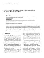
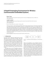
Figure 1: Embedding example.
the algorithm is to change the length of the middle segment
between two successive peaks relative to the total length be-
tween the two peaks so as to be greater or less than a certain
threshold to embed one or zero, respectively. Hence, if the
signal is subject to TSM, then both the middle interval and
the whole segment will change by the same factor leaving the
ratio unchanged. Hence, the algorithm is automatically ro-
bust to TSM without need to rescale the signal. This work
was first introduced in [8].
The average embedding capacity of the algorithm is 20–
30 bps. However, due to practical issues that will be discussed
in Section 3, the embedded data is encoded first with low
code rate. The effective embedding rate drops to 4–6 bps.

The paper is organized as follows. Section 2 describes
the basic idea of the embedding and extraction algorithms.
Section 3 discusses several practical issues and the imple-
mentation details of the general ideas descr ibed in Section 2.
In Section 5, the experimental results of the algorithm are
given.
2. ALGORITHM
2.1. Basic idea
The intervals between a successive maximum and minimum
pair are partitioned to N segments of equal amplitude where
N is odd (typically N = 3or5).Ifwehaveanexactlinear
behavior between the two extrema, then all the segments will
be of equal s ize (up to a quantization error). For sinusoidal-
like segments, the outer segments tend to be longer than the
inner ones because of the smal ler slope at these segments.
If we assume that the total length of the intervals between
the two peaks is L and the length of each segment is l
i
, then
the basic idea of the algorithm is to control the ratio l
(N+1)/2
/L
to be greater or less than a certain threshold γ to embed one
orzero,respectively.TheideaisillustratedinFigure 1.
Note that the smoothness of the signal is increased when
it is lowpass filtered. This results in higher embedding ca-
pacity. However, we need to efficiently reconstruct the sig-
nal from the lowpass component. In our implementation, we
d[−k]
↓2

W1
d[−k]
↓2
W2
Input
c[−k]
↓2
c[−k]
↓2
Approx.
(a) Analysis stage.
W2
↑2 d[k]
W1
↑2 d[ k]
Approx.
↑2 c[k] ↑2 c[k]
Output
(b) Synthesis stage.
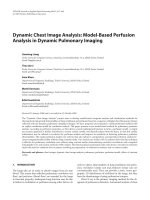
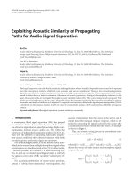
Figure 2: Orthogonal wavelet decomposition.
used a hybrid of orthogonal and nonorthogonal wavelet de-
compositions (as will be discussed in the next subsection) to
satisfy the two requirements of smoothness and efficient re-
construction. The approximation signal at the coarsest scale
is modified rather than the signal itself. The practicalities of
choosing the possible intervals and selecting the threshold
are discussed in Section 3.
2.2. Hybrid orthogonal/nonorthogonal
wavelet decomposition
Therequiredsmoothbehaviordoesnotoccurofteninau-

dio signals except for a set of single-instrument audio like a
piano and a flute. For other composite audio signals, this re-
quirement is hardly fulfilled. This greatly reduces the embed-
ding rate if the original signal is used directly in embedding.
Moreover, even if such a behavior exists, it is very vulnera-
ble to distortion after compression. Hence, the direct audio
signal is not a good candidate for data embedding.
In our implementation, we used a hybrid of orthogonal
and nonorthogonal decompositions. These two types of de-
compositions are illustrated in Figures 2 and 3.
The orthogonal decomposition is an exact (nonredun-
dant) representation of the signal. It involves subsampling
after each decomposition stage. Hence, the approximation
signal is not smoother than the original because of the fre-
quency spread after subsampling. If a modification is done
in the transform domain, then it is preserved after the inverse
and the forward transform because it is nonredundant.
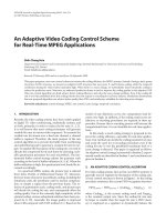
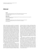
On the other hand, nonorthogonal wavelet decomposi-
tion does not involve subsampling after filtering at each scale,
as illustrated in Figure 3. For our particular pur pose, this de-
composition has a two-fold advantage. First, the lengths are
preserved so that the lengths at any scale are in one-to-one
correspondence with the lengths at the finest scale. The sec-
ond advantage is that the approximation signal at coarser
scales is smoother than the signal at a finer scale.
However, nonorthogonal decomposition is redundant,
that is, not every two dimensional signal is a valid transform.
Hence modification in the transform domain are not guaran-
teed to be preserved if the inverse transform is applied. This
Time-Scale Invariant Audio Data Embedding 995

d
1
[k]
W1
d
1
[k/2]
W2
Input
c
1
[k]
c
1
[k/2]
Approx.
(a) Analysis stage.
W2
d
2
[k/2]
W1
d
2
[k]
Approx.
c
2
[k/2] c
2

[k]
Output
(b) Synthesis stage.
Figure 3: Nonorthogonal wavelet decomposition.
is more apparent if the modification is done at a sufficiently
coarse scale. Hence, at most, two decomposition scales can
be used to embed the data. However, this is not sufficient for
robustness against lossy compression.
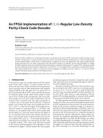
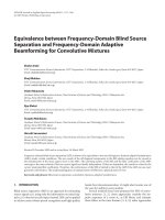
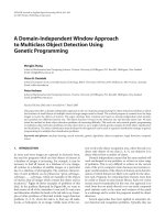
In Figure 4, we illustrate the ideas in the previous two
paragraphs. The first 10
3
samples of the original signals are
plotted along with the approximation signal after three scales
of nonorthogonal and orthogonal decompositions. We no-
tice that the approximation signal after the nonorthogonal
decomposition is much smoother.
In our system, the orthogonal decompositions is applied
first. The resulting approximation signal is further decom-
posed using nonorthogonal decomposition. The orthogonal
decomposition gives the required robustness against lossy
compression but at the cost of reducing the interval lengths,
that is, reducing the embedding rate. The nonorthogonal
decomposition gives the required smooth behavior between
peaks. Typically, one scale of orthogonal decompositions is
used with two scales of nonorthogonal decompositions.
It should be mentioned that the filters of orthogonal and
nonorthogonal decompositions need not be similar. Differ-
ent bases can be used within the same framework. The op-
timality of choosing the wavelet basis for the problem is be-
yond the scope of this paper. However, experimental results

show that different wavelet bases give very comparable re-
sults.
2.3. The embedding algorithm
The first step in the embedding algor ithm is to apply a hy-
brid of orthogonal and nonorthogonal decompositions as
discussed in the previous subsection. After decomposition,
the approximation sig nal at the coarsest scale is used for em-
bedding.
The next step is to change the relative length of the mid-
dle segment between two successive refined extrema to match
the corresponding data bit. Let the total number of samples
Original
After nonorthogonal decomposition
After orthogonal decomposition
Figure 4: Examples of orthogonal and nonorthogonal decomposi-
tions.
between the two extreme points be L and let the length of the
middle segment b e l.Defineα = l/L and the threshold γ.To
embed one, α should be greater than γ, and vice versa. Spline
interpolation is used to modify the lengths. An increase in the
middle segments wil l reflect in a decrease in both of the outer
segments, and vice versa, so as to keep the original length be-
tween the extrema unchanged. Some details for accelerating
the convergence and improving the error performance are
described in Section 3.3 . The overall algorithm is illustrated
in Figure 5.
The main difficulty with the algorithm described above
stems from the redundancy of the nonorthogonal wavelet
transform. Specifically, not all 2D functions are valid wavelet
transform. Therefore, it is possible to end up with a nonvalid

transform after modifying the coarsest scale of the signal. In
particular, some previously used intervals may disappear or
new intervals may arise. This causes a shift in the embedded
sequence from one iteration to another and slows down the
convergence. To partially fix this problem, a repetition code
is used where each bit is repeated an odd number of times
(typically five). The advantage of a repetition code is two-
fold. First, at the encoder side, it accelerates the convergence
because a smaller number of intervals will need modifica-
tion after peak deviation. Second, at the decoder side, it al-
leviates the problem of false alarms as will be discussed later.
The transitions from zero to one and from one to zero are
labeled as markers in the embedded sequence. These mark-
ers play a crucial role in synchronizing the data in the pres-
ence of false alarms and missed peaks as will be described in
Section 4.2.
2.4. The extraction algorithm
The extraction algorithm is straightforward. The hybrid de-
composition is applied as in the encoder. Then, the peaks
996 EURASIP Journal on Applied Signal Processing
Output audio
Signal
reconstruction
Iterate
Identifying
candidate
peaks
Modifying
lengths using
spline

interpolation
Input data
Hybrid orthogonal/
nonorthogonal
wavelet decomposition
Input
audio
Figure 5: Embedding algorithm.
are picked and refined. For the refined intervals, the ratio
α(= l/L)iscalculated.Ifα>γ, then decide one, otherwise
decide zero. If a repetition code is used, then the majority
rule is applied to decide the decoded bit.
This extr action algorithm works well with nice channels,
which do not introduce false alarms or missed data, that
is, channels with no synchronization problems. This type of
channels is a good model for simple operations like volume
change. However, if the audio signal undergoes compression
or lowpass filtering, this ideal situation cannot be assumed
and additional work has to be done to synchronize the data
and remove the false alarms. The details of the practical de-
coding algorithm is discussed in Section 4.3.
3. PRACTICAL ISSUES
3.1. Refining the extrema
The careful selection of the extrema is an important issue in
the algorithm performance. The objective here is to iden-
tify the pairs of successive extrema between which reliable
embedding is possible. The first requirement is to choose
the pairs with distance greater than a certain threshold. This
threshold should guarantee that the middle segment and
each of the outer segments contain at least two samples af-

ter modifying their lengths. The second requirement is that a
refined peak should be a strong one in the sense that it should
be significantly larger (or smaller) than its immediate neigh-
bors. This is important to ensure that the peak will survive
modifications and compression.
Here it is important to mention that adjacent peaks that
are very close to each others and very close to their im-
mediate neighbors are labeled as weak peaks. In our algo-
rithm, weak peaks are not considered peaks at all and they
are ignored if they exist between two successive strong peaks.
Those weak peaks usually arise if the signal undergoes com-
pression. Hence if they are treated as peaks candidates, they
may lead to missed peaks.
3.2. Threshold selection
The selection of the threshold γ is important for the quality
of the output audio and the fast convergence at the encoder.
To minimize the modifications due to changing the length of
the middle interval, we first calculate the histogram of the ra-
tio of the middle segment length to the interval length. Then
we set the threshold as the median of the histogram. This is
done offline only once using a large set of a udio pieces.
3.3. Modifying the lengths
The embedding algorithm as described earlier requires mod-
ification of the lengths of interval segments. For example,
assume we have a data bit of 1, then l/L should be greater
than γ. Otherwise, the length l of the middle segment should
be increased to satisfy this inequality. The increment in the
middle segment reflects in a decrement in both of the outer
segments so as to preserve the original interval length. The
process is reversed for embedding zero. The modification of

all segments is performed via spline inter polation.
To improve the error performance and to give additional
robustness against TSM, a guard band is built around the
threshold so that all modified segments are at least two sam-
ples above or below the threshold value.
The interval lengths should be chosen large enough to
assure that there exists enough number of samples at each
segment after the length decrement. At least two samples are
needed in each segment to perform correct interpolation. For
example, if the intervals are segmented to five levels, then the
typical threshold length between refined peaks is at least 20
samples. This limits the highest-frequency component that
can be used in embedding. For example, if the sampling fre-
quency is 44.1 kHz, and the intervals between two successive
extrema are at least 20 samples, then the highest-frequency
component that is used in embedding is around 1.1 kHz.
Moreover, if an orthogonal decomposition is applied first,
then the subsampling reduces the periods by half at each
scale. Hence, 20 samples after two scales of orthogonal de-
composition corresponds to a frequency of 1.1 kHz/4
≈
275 Hz. For some instruments, these very low frequency
components do not exist, and hence the nonorthogonal
decomposition should be applied on the original signal
directly.
4. ENCODER/DECODER STRUCTURE
Due to the complications introduced by the presence of false
alarms and missed bits, the encoder/decoder structure of the
whole system is more complex than the simple structure de-
scribed earlier. In this section, we will discuss these struc tures

in detail. In the first subsection, we will discuss the source of
false alarms, then we will discuss the encoder/decoder struc-
ture to cope with this problem.
4.1. False alarms
False alarms pose a serious problem for our algorithm and
establish a limitation on the possible embedding r ate. These
false alarms usually arise after mp3 compression. By false
Time-Scale Invariant Audio Data Embedding 997
After
compression
L>Th
Peak
smoothed
Before
compression
L<Th
Strong
peak
Figure 6: False alarms example.
alarms we mean the peaks that are identified by the decoder
but not used by the encoder. These false alarms appear be-
cause of two main reasons.
(1) The smoothing effect of compression and lowpass fil-
tering. This may remove some weak peaks.
(2) The deviation of some strong peaks at the threshold
length after signal processing. For example, assume
that refined peaks should be 30 samples apart, then at
the encoder peaks that are 29 samples apart are not
considered in embedding. However, these periods may
increaseaftercompressionbyonesample(ormore).

Therefore, the decoder will recognize them as ac tive
periods.
These two sources of false alarms are illustrated in
Figure 6.
These false alarms lead to a loss in synchronization at the
decoder. Remedies for this problem are treated in Sections
4.2 and 4.3. The problem was treated in detail in [9, 10].
It should be mentioned that missed peaks might also take
place. However, this happens much less frequently than the
false alarms. The number of false alarms that arise ranges
from 2% to 15% of the total number of peaks depending on
the nature of the audio signal.
4.2. Encoding
To alleviate the problem of false alarms, a self-synchroni-
zation mechanism should be contained in the embedded se-
quence. As mentioned earlier, a repetition code is used at the
encoder to improve the convergence and the error perfor-
mance. If each bit is repeated r times and a single false alarm
occurs within a sequence of r similar bits, then it can be easily
identified and removed.
The main idea of the encoding algorithm is to isolate the
false alarms so as to identify them individually. At each tran-
sition from a group of ones to a group of zeros (or the re-
verse), a marker is put. The sequence of bits between succes-
sive markers are decoded separately. In [8], long sequences of
zeros or ones are cut by employing high-density bipolar cod-
ing (HDBn) scheme in digital communication to add a bit
of reverse polarity to a long sequence of similar bits. How-
ever, experiments show that this may lead to loss of synchro-
nization in the extracted bits if the extra bit is not identified

properly.
4.3. Decoding
The decoder performs the following steps.
(1) Extract ing the embedded bit as described in Section
2.4. During extraction, each bit is given a score that
represents the certainty about the correctness of this
bit. The higher the score, the higher the certainty of the
corresponding bit. This score is s imply the difference
between the actual length of the middle segment and
the threshold length. These scores are used in further
operations.
(2) Applying a median filter (with width = r) to the ex-
tracted bits sequence so as to remove sparse bits that
do not agree with their neighbors, and at the same
time preserving the correct transition between differ-
ent bits.
(3) Identifying the markers, which are defined as the
points at which a sign change occurs, and the median
of its following bits is different from that of the preced-
ing bits.
(4) Identifying the bit sequence between the markers. If
the number of bits is divisible by r, then the sequence
of bits is decoded using the majority rule. The prob-
lems arise when the number of bits between two suc-
cessive markers is not divisible by r. For example, as-
sume r = 5 and the number of bits between two suc-
cessive markers is 13, then we have two possibilities.
The first possibility is that the correct number of bits is
10, and we have three false alarms; the other is that the
correct number is 15 and we have two missed peaks.

The decision between the two possibilities is based on
the scores of the residual bits, that is, the three bits with
the lowest scores. If the average score of these bits is
far s maller than the average of the remaining bits, then
they are classified as false alarms, otherwise, they are
classified as missed peaks.
(5) Remove the redundant bits that are added at the en-
coder side if HDBn encoding is employed. This is done
by skipping a bit with opposite sign that follows n sim-
ilar bits in the final output stream.
In what follows, we will discuss the effect of repetition
encoding in reducing the probability of false alarms. We will
use the following assumptions.
(1) Only false alarms exist (no missed bit).
(2) The probability of false alarms is P
f
.
(3) False alarm events are indep endent.
(4) Each bit is repeated r times.
(5) All markers are identified correctly.
(6) The number of false alarms between two markers is
less than the number of the original bits between them.
998 EURASIP Journal on Applied Signal Processing
Table 1: Probabilities of the number of bits between markers.
Bits before encoding Bits after encoding Probability
1 r 1/2
22r 1/4
.
.
.

.
.
.
.
.
.
nnr1/2
n
.
.
.
.
.
.
.
.
.
After repetition, a false alarm exists if there are more than
(r +1)/2 false alarms between two successive markers. With
repetition, we can have multiple of r bits between two suc-
cessive markers. If zero and one are equally probable, then
Table 1 gives the probabilities for the number of bits between
markers.
The number of false alarms within a given number of bits
has a binomial distribution because the false-alarm events are
independent. The probability of having k false alarms in a
sample space of size N bits is
P
N
(k) =


N
k

P
k
f

1 − P
f

N−k
. (1)
Note that in (1) N takes the discrete values r, 2r, 3r, ,andso
forth. The probability of having a false alarm after encoding
is the probability of having N/2 false alarms or more be-
tween two successive markers, where · is the ceiling integer
function. Hence the new probability of false alarm is
P
FA
=
∞

m=1
mr

k=mr/2
P
mr
(k)


1
2

m
,
P
FA
=
∞

m=1
mr

k=mr/2

mr
k

P
k
f

1 − P
f

mr−k

1
2


m
(2)
In Figure 7, we show the reduction in the probability of
false alarms after using repetition encoding with n = 3, 5, 7.
Note that, for the typical range of P
f
(between 0.1 and 0.2),
the range of P
FA
is between 0.01 and 0.05. This range of false
alarms is quite adequate for the algor ithms described in [9,
10]toworkefficiently with high code rate, for example, 2/3.
These algorithms are based on novel decoding techniques for
the common convolutional codes.
The overall encoder system consists of a frontend of con-
volution encoder followed by the repetition encoder which
simply repeat each bit for r times. At the decoder side, the
repetition decoder (with majority decision rule) is applied on
the extracted data, then the convolutional decoder is applied
to take care of the residual false alarms. The overall system is
shown in Figure 8.
5. EXPERIMENTAL RESULTS
The algorithm was applied to a set of 13 audio signals. The
lengths of the sequences were around 11 seconds. The test
Input false alarm probability
00.10.20.30.40.50.60.70.80.91
Output false alarm probability
0
0.1

0.2
0.3
0.4
0.5
0.6
0.7
0.8
0.9
1
r =3
r =5
r =7
Figure 7: Coding gain after repetition.
Input
data
Convolutional
encoder
Repetition
encoder
Bits
embedding
Modified
audio
Input audio
(a) Encoder.
Input
audio
Bits
extraction
Repetition

decoder
Convolutional
decoder
Output
data
(b) Decoder.
Figure 8: Overall encoding/decoding structure.
signals include speech, single instrument music (piano, flute,
and violin), and composite music. All test signals are mono
with sampling rate 44.1 kHz. In all the experiments, we use
Daubechies db5 wavelet for orthogonal decomposition, and
the derivative of cubic spline wavelet [11] for nonorthogonal
decomposition.
The number of levels between two successive extrema is
chosen to be an odd number so that the middle segment is
usually symmetric around zero. Therefore, the largest mod-
ification, which takes place in the middle segment, is in the
lowest amplitude region. The typical choice is three or five
levels. The larger the number of levels, the better the er-
ror performance. However, the output quality (although still
high in al l cases) is higher with lower number of levels be-
cause no large changes occur in this case. It was found that
the choice of three levels and interval l ength of 40 samples
gives the best compromise between quality and robustness.
This parameter setting is used in all the following tests.
(i) Embedding rate. The median embedding rate of the
uncoded data is around 25 bps. However, after coding,
the effective embedding rate becomes 5 bps. The em-
bedding ra te is very large for single instruments, where
pure sinusoids with low frequencies are dominant. The

Time-Scale Invariant Audio Data Embedding 999
Table 2: Performance versus signal processing operations.
Operation Insertions Deletions Errors
mp3 compression 0.039 0.0065 0.018
LPF ( 4 kHz) 0.019 0.005 0.003
Adding noise (36 dB) 0.001 0.001 0
Resampling to 48 kHz 0.002 0.013 0
embedding rates of the algorithm depend heavily on
the signal nature. If the signal contains long intervals
of low frequencies, then the embedding rate increases
significantly. It can be as high as 80 bps for the above
parameter setting.
(ii) Noiseless channel. The algor ithm described in Sec-
tions 2.3 and 2.4 worksperfectlywithallsequences.
However, sometimes, especially with speech signals, it
needs an excessive number of iterations at the encoder
to converge.
(iii) Quality. The quality of the output signal is very high,
and for a nonprofessional listener, it is very hard to
distinguish between the original and modified signals.
However, when the algorithm was tested with speech
signals, the results were not satisfactory.
(iv) Time shift and cropping. The proposed algorithm is au-
tomatically robust to time shift and cropping. How-
ever, for time cropping, some bits may be missed if
a modified interval is cropped. This is unlikely to
occur because the intervals used in embedding are
usually active audio intervals. If such intervals are
cropped, this will affect the audio content. More-
over, with repetition code, deletions can be com-

pensated. However, this can be done only for r an-
dom deletions. To randomize the effect of time crop-
ping, bit interleaver may be used prior to repetition
encoding.
(v) mp3 compression. We tested the performance of the
system against mp3 compression with rates 112 kbps
(compression ratio 6.3 : 1). The average rates are
shown in Tabl e 2. These rates are well suited to the al-
gorithm described in [10]toworkefficiently. However,
at lower compression bit rate, the insertions rate tends
to increase significantly.
(vi) Lowpass filtering. Due to the lowpass component of the
approximation signal, the algorithm is robust to low-
pass filtering. The typical rates are shown in Table 2 .
(vii) Time-scale modification. This is the most powerful fea-
ture of the proposed algorithm. It is automatically ro-
bust to TSM up to a quantization error factor. This
means that false alarms (or missed bits) may ap-
pear because of the rounding of the thresholds. Con-
sider, for example, if the threshold before TSM is
40, and the time-scale factor is 0.96, then the new
length becomes 38.4. Then we have two choices for
the threshold length (which should be integer), ei-
ther 38 or 39. The smaller choice may result in false
Table 3: Performance versus TSM.
Factor Insertions Deletions Errors
0.96 0.068 0 0.018
0.98 0.044 0 0.011
1.02 0.023 0.006 0.006
1.04 0.004 0.012 0

alarms while the larger one may cause missed bits. In
Table 3 , we show the performance of the algorithm
versus different fac tors of time-scale modifications. In
this table, the new threshold length is the round of
the old threshold length multiplied by the time-scale
factor.
(viii) It should be mentioned that, in the above results, we
assumed a fixed time-scale factor. The algorithm can
be made robust to time-varying TSM if the thresh-
old of the interval lengths is adaptively updated. From
Table 3 , it is noticed that either insertions or deletions
are dominant at different scale factors. This depends
on the rounding. If it is to the smaller integer, then
insertions will be more frequent and vice versa. Note
that the algorithm is also automatically robust to re-
sampling by any factor. In Table 2 , we show the per-
formance against resampling to 48 kHz. It should be
mentioned that, for dyadic resampling or upsampling ,
we may need to reduce the number of decomposition
levels at the decoder to match the levels before resam-
pling.
The robustness of the proposed algorithm against
mp3 compression and other signal processing operations
is comparable to the results reported in recent audio
spread-spectrum watermarking works (e.g., [12, 13]) and
projection-based watermarking schemes (e.g., [14]), where
the bit error rate is between 0.001 and 0.03. However, TSM
and synchronization attacks have not been studied for most
audio watermarking algorithms proposed in the literature
because such attacks cannot be compensated within the tra-

ditional frameworks. Robustness to these attacks is the main
strength of the proposed algorithm.
6. CONCLUSION
In this work, we propose a novel algorithm for embedding
data in audio by changing the interval length of certain seg-
ments of the audio signal. The algorithm is invariant after
TSM, time shift, and time cropping. We proposed a set of
encoding and decoding techniques to survive the common
mp3 compression.
The embedding rate of the algorithm is above 20 bps.
However, as discussed for practical reasons, repetition cod-
ing is used and the effective embedding rate is 4–8 bps. The
quality of the output is very high and it is indistinguishable
from the original signal.
1000 EURASIP Journal on Applied Signal Processing
The proposed technique is suitable for applications like
broadcast monitoring, where the embedded data are infor-
mation relevant to host signal and used for several purposes,
for example, tracking the use of the signal, providing statisti-
cal data collection, and analyzing the broadcast content.
REFERENCES
[1] P. Bassia, I. Pitas, and N. Nikolaidis, “Robust audio water-
marking in the time domain,” IEEE Trans. Multimedia, vol. 3,
no. 2, pp. 232–241, 2001.
[2] W. Bender, D. Gruhl, N. Morimoto, and A. Lu, “Techniques
for data hiding,” IBM Systems Journal,vol.35,no.3-4,pp.
313–336, 1996.
[3] J. F. Tilki and A. Beex, “Encoding a hidden digital signa-
ture onto an audio signal using psychoacoustic masking,” in
Proc. 7th International Conference on Signal Processing Ap-

plications and Technology, pp. 476–480, Boston, Mass, USA,
1996.
[4] S. K. Lee and Y. S. Ho, “Digital audio watermarking in the
cepstrum domain,” in Proc. IEEE International Conference on
Consumer Electronics, pp. 334–335, Los Angeles, Calif, USA,
2000.
[5] D. Kirovski and H. Malvar, “Robust spread-spectrum au-
dio watermarking,” in Proc. IEEE Int. Conf. Acoustics, Speech,
Signal Processing, vol. 3, pp. 1345–1348, Salt Lake City, Utah,
USA, 2001.
[6] M. D. Swanson, B. Zhu, and A. H. Tewfik, “Data hiding for
video-in-video,” in Proceedings of IEEE International Con-
ference on Image Processing, vol. 2, pp. 676–679, Washington,
DC, USA, 1997.
[7] M. F. Mansour and A. H. Tewfik, “Audio watermarking by
time-scale modification,” in Proc. IEEE Int. Conf. Acoustics,
Speech, Signal Processing, vol. 3, pp. 1353–1356, Salt Lake City,
Utah, USA, 2001.
[8] M. F. Mansour and A. H. Tewfik, “Time-scale invariant audio
data embedding,” in Proc. IEEE International Conference on
Multimedia and Expo, Tokyo, Japan, 2001.
[9] M.F.MansourandA.H.Tewfik, “Efficient decoding of wa-
termarking schemes in the presence of false alarms,” in Proc.
IEEE 4th Workshop on Multimedia Signal Processing, pp. 523–
528, Cannes, France, 2001.
[10] M. F. Mansour and A. H. Tewfik, “Convolutional decoding for
channels with false alarms,” in Proc. IEEE Int. Conf. Acoustics,
Speech, Signal Processing, vol. 3, pp. 2501–2504, Orlando, Fla,
USA, 2002.
[11] S. Mallat, A Wavelet Tour of Signal Processing, Academic Press,

Boston, Mass, USA, 2nd edition, 1999.
[12] J. W. Seok and J. W. Hong, “Audio watermarking for copyright
protection of digital audio data,” Electronics Letters, vol. 37,
no. 1, pp. 60–61, 2001.
[13] G. C. M. Silvestre, N. J. Hurley, G. S. Hanau, and W. J. Dowl-
ing, “Informed audio watermarking scheme using digital
chaotic signals,” in Proc. IEEE Int. Conf. Acoustics, Speech,
Signal Processing, vol. 3, pp. 1361–1364, Salt Lake City, Utah,
USA, 2001.
[14] M. D. Swanson, B. Zhu, and A. H. Tewfik, “Current state
of the art, challenges and future directions for audio wa-
termarking,” in IEEE Internat ional Conference on Multime-
dia Computing and Systems, vol. 1, pp. 19–24, Florence, Italy,
1999.
Mohamed F. Mansour was born in Cairo, Egypt, in 1973. He re-
ceived his B.S. and M.S. degrees from Cairo University, Cairo,
Egypt, in 1995 and 1998, respectively, and his Ph.D. degree from
the University of Minnesota, Minneapolis, Minn, in 2003, all in
electrical engineering. During the period 1999–2003, he was with
the Department of Electrical and Computer Engineering, Univer-
sity of Minnesota as a Research and Teaching Assistant. In 2003,
he joined DSPS R&D Center at Texas Instruments Inc., Dallas, Tex,
as a member of technical staff. His current research interests are in
real-time signal processing, adaptive filtering, and optimization.
Ahmed H. Tewfik received his B.S. degree from Cairo University,
Cairo, Egypt, in 1982 and his M.S., E.E., and S.D. degrees from the
Massachusetts Institute of Technology, Cambridge, MA, in 1984,
1985, and 1987, respectively. Dr. Tewfik has worked at Alphatech,
Inc., Burlington, MA, in 1987. He is the E. F. Johnson Professor
of Electronic Communications with the Department of Electrical

Engineering at the University of Minnesota. He ser ved as a Consul-
tant to MTS Systems, Inc., Eden Prairie, MN and Rosemount, Inc.,
Eden Prairie, MN and worked with Texas Instruments and Com-
puting Devices International. From August 1997 to August 2001,
he was the President and CEO of Cognicity, Inc., an entertainment
marketing software tools publisher t hat he co-founded. Dr. Tewfik
is a Fellow of the IEEE. He was a Distinguished Lecturer of the IEEE
Signal Processing Society in 1997–1999. He received the IEEE Third
Millennium Award in 2000.