Quantum Mechanics For Electrical Engineers

QUANTUM MECHANICS
FOR ELECTRICAL
ENGINEERS
IEEE Press
445 Hoes Lane
Piscataway, NJ 08854
IEEE Press Editorial Board
Lajos Hanzo, Editor in Chief
R. Abhari M. El - Hawary O. P. Malik
J. Anderson B - M. Haemmerli S. Nahavandi
G. W. Arnold M. Lanzerotti T. Samad
F. Canavero D. Jacobson G. Zobrist
Kenneth Moore, Director of IEEE Book and Information Services (BIS)
Technical Reviewers
Prof. Richard Ziolkowski, University of Arizona
Prof. F. Marty Ytreberg, University of Idaho
Prof. David Citrin, Georgia Institute of Technology
Prof. Steven Hughes, Queens University
QUANTUM MECHANICS
FOR ELECTRICAL
ENGINEERS
DENNIS M. SULLIVAN
A JOHN WILEY & SONS, INC., PUBLICATION
IEEE PRESS
IEEE Series on Microelectronics Systems
Jake Baker, Series Editor
Copyright © 2012 by the Institute of Electrical and Electronics Engineers, Inc.
Published by John Wiley & Sons, Inc., Hoboken, New Jersey. All rights reserved.
Published simultaneously in Canada
MATLAB and Simulink are registered trademarks of The MathWorks, Inc. See www.

mathworks.com/trademarks for a list of additional trade marks. The MathWorks Publisher
Logo identifi es books that contain MATLAB® content. Used with permission. The MathWorks
does not warrant the accuracy of the text or exercises in this book or in the software
downloadable from
and leexchage/?term=authored%3A80973. The
book’s or downloadable software’s use or discussion of MATLAB® software or related
products does not constitute endorsement or sponsorship by The MathWorks of a particular
use of the MATLAB® software or related products.
For MATLAB® and Simulink® product information, in information on other related products,
please contact:
The MathWorks, Inc.
3 Apple Hill Drive
Natick, MA 01760-2098 USA
Tel: 508-647-7000
Fax: 508-647-7001
E-mail:
Web: www.mathworks.com
No part of this publication may be reproduced, stored in a retrieval system, or transmitted in
any form or by any means, electronic, mechanical, photocopying, recording, scanning, or
otherwise, except as permitted under Section 107 or 108 of the 1976 United States Copyright
Act, without either the prior written permission of the Publisher, or authorization through
payment of the appropriate per-copy fee to the Copyright Clearance Center, Inc., 222
Rosewood Drive, Danvers, MA 01923, (978) 750-8400, fax (978) 750-4470, or on the web at
www.copyright.com. Requests to the Publisher for permission should be addressed to the
Permissions Department, John Wiley & Sons, Inc., 111 River Street, Hoboken, NJ 07030,
(201) 748-6011, fax (201) 748-6008, or online at />Limit of Liability/Disclaimer of Warranty: While the publisher and author have used their best
efforts in preparing this book, they make no representations or warranties with respect to the
accuracy or completeness of the contents of this book and specifi cally disclaim any implied
warranties of merchantability or fi tness for a particular purpose. No warranty may be created
or extended by sales representatives or written sales materials. The advice and strategies

contained herein may not be suitable for your situation. You should consult with a professional
where appropriate. Neither the publisher nor author shall be liable for any loss of profi t or any
other commercial damages, including but not limited to special, incidental, consequential, or
other damages.
For general information on our other products and services or for technical support, please
contact our Customer Care Department within the United States at (800) 762-2974, outside the
United States at (317) 572-3993 or fax (317) 572-4002.
Wiley also publishes its books in a variety of electronic formats. Some content that appears in
print may not be available in electronic formats. For more information about Wiley products,
visit our web site at www.wiley.com.
Library of Congress Cataloging-in-Publication Data
ISBN: 978-0-470-87409-7
Printed in the United States of America
10 9 8 7 6 5 4 3 2 1
T o
My Girl
CONTENTS
vii
Preface xiii
Acknowledgments xv
About the Author xvii
1. Introduction 1
1.1 Why Quantum Mechanics?, 1
1.1.1 Photoelectric Effect, 1
1.1.2 Wave–Particle Duality, 2
1.1.3 Energy Equations, 3
1.1.4 The Schrödinger Equation, 5
1.2 Simulation of the One-Dimensional, Time-Dependent
Schrödinger Equation, 7
1.2.1 Propagation of a Particle in Free Space, 8

1.2.2 Propagation of a Particle Interacting with a Potential, 11
1.3 Physical Parameters: The Observables, 14
1.4 The Potential V(x), 17
1.4.1 The Conduction Band of a Semiconductor, 17
1.4.2 A Particle in an Electric Field, 17
1.5 Propagating through Potential Barriers, 20
1.6 Summary, 23
Exercises, 24
References, 25
viii CONTENTS
2. Stationary States 27
2.1 The Infi nite Well, 28
2.1.1 Eigenstates and Eigenenergies, 30
2.1.2 Quantization, 33
2.2 Eigenfunction Decomposition, 34
2.3 Periodic Boundary Conditions, 38
2.4 Eigenfunctions for Arbitrarily Shaped Potentials, 39
2.5 Coupled Wells, 41
2.6 Bra-ket Notation, 44
2.7 Summary, 47
Exercises, 47
References, 49
3. Fourier Theory in Quantum Mechanics 51
3.1 The Fourier Transform, 51
3.2 Fourier Analysis and Available States, 55
3.3 Uncertainty, 59
3.4 Transmission via FFT, 62
3.5 Summary, 66
Exercises, 67
References, 69

4. Matrix Algebra in Quantum Mechanics 71
4.1 Vector and Matrix Representation, 71
4.1.1 State Variables as Vectors, 71
4.1.2 Operators as Matrices, 73
4.2 Matrix Representation of the Hamiltonian, 76
4.2.1 Finding the Eigenvalues and Eigenvectors of a Matrix, 77
4.2.2 A Well with Periodic Boundary Conditions, 77
4.2.3 The Harmonic Oscillator, 80
4.3 The Eigenspace Representation, 81
4.4 Formalism, 83
4.4.1 Hermitian Operators, 83
4.4.2 Function Spaces, 84
Appendix: Review of Matrix Algebra, 85
Exercises, 88
References, 90
5. A Brief Introduction to Statistical Mechanics 91
5.1 Density of States, 91
5.1.1 One-Dimensional Density of States, 92
5.1.2 Two-Dimensional Density of States, 94
5.1.3 Three-Dimensional Density of States, 96
5.1.4 The Density of States in the Conduction Band of a
Semiconductor, 97
CONTENTS ix
5.2 Probability Distributions, 98
5.2.1 Fermions versus Classical Particles, 98
5.2.2 Probability Distributions as a Function of Energy, 99
5.2.3 Distribution of Fermion Balls, 101
5.2.4 Particles in the One-Dimensional Infi nite Well, 105
5.2.5 Boltzmann Approximation, 106
5.3 The Equilibrium Distribution of Electrons and Holes, 107

5.4 The Electron Density and the Density Matrix, 110
5.4.1 The Density Matrix, 111
Exercises, 113
References, 114
6. Bands and Subbands 115
6.1 Bands in Semiconductors, 115
6.2 The Effective Mass, 118
6.3 Modes (Subbands) in Quantum Structures, 123
Exercises, 128
References, 129
7. The Schrödinger Equation for Spin-1/2 Fermions 131
7.1 Spin in Fermions, 131
7.1.1 Spinors in Three Dimensions, 132
7.1.2 The Pauli Spin Matrices, 135
7.1.3 Simulation of Spin, 136
7.2 An Electron in a Magnetic Field, 142
7.3 A Charged Particle Moving in Combined E and B Fields, 146
7.4 The Hartree–Fock Approximation, 148
7.4.1 The Hartree Term, 148
7.4.2 The Fock Term, 153
Exercises, 155
References, 157
8. The Green’s Function Formulation 159
8.1 Introduction, 160
8.2 The Density Matrix and the Spectral Matrix, 161
8.3 The Matrix Version of the Green’s Function, 164
8.3.1 Eigenfunction Representation of Green’s
Function, 165
8.3.2 Real Space Representation of Green’s Function, 167
8.4 The Self-Energy Matrix, 169

8.4.1 An Electric Field across the Channel, 174
8.4.2 A Short Discussion on Contacts, 175
Exercises, 176
References, 176
x CONTENTS
9. Transmission 177
9.1 The Single-Energy Channel, 177
9.2 Current Flow, 179
9.3 The Transmission Matrix, 181
9.3.1 Flow into the Channel, 183
9.3.2 Flow out of the Channel, 184
9.3.3 Transmission, 185
9.3.4 Determining Current Flow, 186
9.4 Conductance, 189
9.5 Büttiker Probes, 191
9.6 A Simulation Example, 194
Exercises, 196
References, 197
10. Approximation Methods 199
10.1 The Variational Method, 199
10.2 Nondegenerate Perturbation Theory, 202
10.2.1 First-Order Corrections, 203
10.2.2 Second-Order Corrections, 206
10.3 Degenerate Perturbation Theory, 206
10.4 Time-Dependent Perturbation Theory, 209
10.4.1 An Electric Field Added to an Infi nite Well, 212
10.4.2 Sinusoidal Perturbations, 213
10.4.3 Absorption, Emission, and Stimulated Emission, 215
10.4.4 Calculation of Sinusoidal Perturbations Using
Fourier Theory, 216

10.4.5 Fermi’s Golden Rule, 221
Exercises, 223
References, 225
11. The Harmonic Oscillator 227
11.1 The Harmonic Oscillator in One Dimension, 227
11.1.1 Illustration of the Harmonic Oscillator Eigenfunctions, 232
11.1.2 Compatible Observables, 233
11.2 The Coherent State of the Harmonic Oscillator, 233
11.2.1 The Superposition of Two Eigentates in an Infi nite
Well, 234
11.2.2 The Superposition of Four Eigenstates in a Harmonic
Oscillator, 235
11.2.3 The Coherent State, 236
11.3 The Two-Dimensional Harmonic Oscillator, 238
11.3.1 The Simulation of a Quantum Dot, 238
Exercises, 244
References, 244
CONTENTS xi
12. Finding Eigenfunctions Using Time-Domain Simulation 245
12.1 Finding the Eigenenergies and Eigenfunctions in One
Dimension, 245
12.1.1 Finding the Eigenfunctions, 248
12.2 Finding the Eigenfunctions of Two-Dimensional Structures, 249
12.2.1 Finding the Eigenfunctions in an Irregular Structure, 252
12.3 Finding a Complete Set of Eigenfunctions, 257
Exercises, 259
References, 259
Appendix A. Important Constants and Units 261
Appendix B. Fourier Analysis and the Fast Fourier Transform (FFT) 265
B.1 The Structure of the FFT, 265

B.2 Windowing, 267
B.3 FFT of the State Variable, 270
Exercises, 271
References, 271
Appendix C. An Introduction to the Green’s Function Method 273
C.1 A One-Dimensional Electromagnetic Cavity, 275
Exercises, 279
References, 279
Appendix D. Listings of the Programs Used in this Book 281
D.1 Chapter 1, 281
D.2 Chapter 2, 284
D.3 Chapter 3, 295
D.4 Chapter 4, 309
D.5 Chapter 5, 312
D.6 Chapter 6, 314
D.7 Chapter 7, 323
D.8 Chapter 8, 336
D.9 Chapter 9, 345
D.10 Chapter 10, 356
D.11 Chapter 11, 378
D.12 Chapter 12, 395
D.13 Appendix B, 415
Index 419
MATLAB Coes are downloadable from
PREFACE
xiii
A physics professor once told me that electrical engineers were avoiding learn-
ing quantum mechanics as long as possible. The day of reckoning has arrived.
Any electrical engineer hoping to work in the fi eld of modern semiconductors
will have to understand some quantum mechanics.

Quantum mechanics is not normally part of the electrical engineering
curriculum. An electrical engineering student taking quantum mechanics
in the physics department may fi nd it to be a discouraging experience. A
quantum mechanics class often has subjects such as statistical mechanics,
thermodynamics, or advanced mechanics as prerequisites. Furthermore, there
is a greater cultural difference between engineers and physicists than one
might imagine.
This book grew out of a one - semester class at the University of Idaho titled
“ Semiconductor Theory, ” which is actually a crash course in quantum mechan-
ics for electrical engineers. In it there are brief discussions on statistical
mechanics and the topics that are needed for quantum mechanics. Mostly, it
centers on quantum mechanics as it applies to transport in semiconductors. It
differs from most books in quantum mechanics in two other very important
aspects: (1) It makes use of Fourier theory to explain several concepts, because
Fourier theory is a central part of electrical engineering. (2) It uses a simula-
tion method called the fi nite - difference time - domain (FDTD) method to
simulate the Schr ö dinger equation and thereby provides a method of illustrat-
ing the behavior of an electron. The simulation method is also used in the
exercises. At the same time, many topics that are normally covered in an
introductory quantum mechanics text, such as angular momentum, are not
covered in this book.
xiv PREFACE
THE LAYOUT OF THE BOOK
Intended primarily for electrical engineers, this book focuses on a study of
quantum mechanics that will enable a better understanding of semiconductors.
Chapters 1 through 7 are primarily fundamental topics in quantum mechanics.
Chapters 8 and 9 deal with the Green ’ s function formulation for transport in
semiconductors and are based on the pioneering work of Supriyo Datta and
his colleagues at Purdue University. The Green ’ s function is a method for
calculating transport through a channel. Chapter 10 deals with approximation

methods in quantum mechanics. Chapter 11 talks about the harmonic oscilla-
tor, which is used to introduce the idea of creation and annihilation operators
that are not otherwise used in this book. Chapter 12 describes a simulation
method to determine the eigenenergies and eigenstates in complex structures
that do not lend themselves to easy analysis.
THE SIMULATION PROGRAMS
Many of the fi gures in this book have a title across the top. This title is the
name of the MATLAB program that was used to generate that fi gure. These
programs are available to the reader. Appendix D lists all the programs, but
they can also be obtained from the following Internet site:
.
The reader will fi nd it benefi cial to use these programs to duplicate the fi gures
and perhaps explore further. In some cases the programs must be used to
complete the exercises at the end of the chapters. Many of the programs are
time - domain simulations using the FDTD method, and they illustrate the
behavior of an electron in time. Most readers fi nd these programs to be
extremely benefi cial in acquiring some intuition for quantum mechanics. A
request for the solutions manual needs to be emailed to .
D ennis M. S ullivan
Department of Electrical and Computer Engineering
University of Idaho
ACKNOWLEDGMENTS
xv
I am deeply indebted to Prof. Supriyo Datta of Purdue University for his help,
not only in preparing this book, but in developing the class that led to the
book. I am very grateful to the following people for their expertise in editing
this book: Prof. Richard Ziolkowski from the University of Arizona; Prof. Fred
Barlow, Prof. F. Marty Ytreberg, and Paul Wilson from the University of Idaho;
Prof. David Citrin from the Georgia Institute of Technology; Prof. Steven
Hughes from Queens University; Prof. Enrique Navarro from the University

of Valencia; and Dr. Alexey Maslov from Canon U.S.A. I am grateful for the
support of my department chairman, Prof. Brian Johnson, while writing this
book. Mr. Ray Anderson provided invaluable technical support. I am also very
grateful to Ms. Judy LaLonde for her editorial assistance.
D.M.S.
ABOUT THE AUTHOR
xvii
Dennis M. Sullivan graduated from Marmion Military Academy in Aurora,
Illinois in 1966. He spent the next 3 years in the army, including a year as an
artillery forward observer with the 173rd Airborne Brigade in Vietnam. He
graduated from the University of Illinois with a bachelor of science degree in
electrical engineering in 1973, and received master ’ s degrees in electrical engi-
neering and computer science from the University of Utah in 1978 and 1980,
respectively. He received his Ph.D. degree in electrical engineering from the
University of Utah in 1987.
From 1987 to 1993, he was a research engineer with the Department of
Radiation Oncology at Stanford University, where he developed a treatment
planning system for hyperthermia cancer therapy. Since 1993, he has been on
the faculty of electrical and computer engineering at the University of Idaho.
His main interests are electromagnetic and quantum simulation. In 1997, his
paper “ Z Transform Theory and the FDTD Method, ” won the R. P. W. King
Award from the IEEE Antennas and Propagation Society. In 2001, he received
a master ’ s degree in physics from Washington State University while on sab-
batical leave. He is the author of the book Electromagnetic Simulation Using
the FDTD Method , also from IEEE Press.
1
INTRODUCTION
1
This chapter serves as a foundation for the rest of the book. Section 1.1 pro-
vides a brief history of the physical observations that led to the development

of the Schr ö dinger equation, which is at the heart of quantum mechanics.
Section 1.2 describes a time - domain simulation method that will be used
throughout the book as a means of understanding the Schr ö dinger equation.
A few examples are given. Section 1.3 explains the concept of observables, the
operators that are used in quantum mechanics to extract physical quantities
from the Schr ö dinger equation. Section 1.4 describes the potential that is the
means by which the Schr ö dinger equation models materials or external infl u-
ences. Many of the concepts of this chapter are illustrated in Section 1.5 , where
the simulation method is used to model an electron interacting with a barrier.
1.1 WHY QUANTUM MECHANICS?
In the late nineteenth century and into the fi rst part of the twentieth century,
physicists observed behavior that could not be explained by classical mechan-
ics [1] . Two experiments in particular stand out.
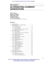
1.1.1 Photoelectric Effect
When monochromatic light — that is, light at just one wavelength — is used to
illuminate some materials under certain conditions, electrons are emitted from
Quantum Mechanics for Electrical Engineers, First Edition. Dennis M. Sullivan.
© 2012 The Institute of Electrical and Electronics Engineers, Inc.
Published 2012 by John Wiley & Sons, Inc.
2 1 INTRODUCTION
the material. Classical physics dictates that the energy of the emitted particles
is dependent on the intensity of the incident light. Instead, it was determined
that at a constant intensity, the kinetic energy (KE) of emitted electrons varies
linearly with the frequency of the incident light (Fig. 1.1 ) according to:

Ehf−=
φ
,
where, ϕ , the work function, is the minimum energy that the particle needs to
leave the material.

Planck postulated that energy is contained in discrete packets called quanta,
and this energy is related to frequency through what is now known as Planck ’ s
constant, where h = 6.625 × 1 0
− 34
J · s,

Ehf= .
(1.1)
Einstein suggested that the energy of the light is contained in discrete wave
packets called photons. This theory explains why the electrons absorbed spe-
cifi c levels of energy dictated by the frequency of the incoming light and
became known as the photoelectric effect.
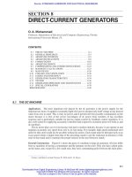
1.1.2 Wave – Particle Duality
Another famous experiment suggested that particles have wave properties.
When a source of particles is accelerated toward a screen with a single opening,
a detection board on the other side shows the particles centered on a position
right behind the opening as expected (Fig. 1.2 a). However, if the experiment
is repeated with two openings, the pattern on the detection board suggests
points of constructive and destructive interference, similar to an electromag-
netic or acoustic wave (Fig. 1.2 b).
FIGURE 1.1 The photoelectric effect. (a) If certain materials are irradiated with light,
electrons within the material can absorb energy and escape the material. (b) It was
observed that the KE of the escaping electron depends on the frequency of the light.
(a) (b)
Incident light
at frequency f
Frequency
f
f
Max. kinetic energy

Emitted electrons
with energy E - φ=hf.
1.1 WHY QUANTUM MECHANICS? 3
Based on observations like these, Louis De Broglie postulated that matter
has wave - like qualities. According to De Broglie, the momentum of a particle
is given by:

p
h
=
λ
,
(1.2)
where λ is the wavelength. Observations like Equations (1.1) and (1.2) led to
the development of quantum mechanics.
1.1.3 Energy Equations
Before actually delving into quantum mechanics, consider the formulation of a
simple energy problem. Look at the situation illustrated in Figure 1.3 and think
about the following problem: If the block is nudged onto the incline and rolls to
the bottom, what is its velocity as it approaches the fl at area, assuming that we
FIGURE 1.2 The wave nature of particles. (a) If a source of particles is directed at
a screen with one opening, the distribution on the other side is centered at the opening,
as expected. (b) If the screen contains two openings, points of constructive and destruc-
tive interference are observed, suggesting a wave.
Particle
source
(a) (b)
Particle
source
FIGURE 1.3 (a) A block with a mass of 1 kg has been raised 1 m. It has a PE of 9.8 J.

(b) The block rolls down the frictionless incline. Its entire PE has been turned into KE.
(a) (b)
1 m
v
1 kg
g = 9.8 m/s
2
4 1 INTRODUCTION
can ignore friction? We can take a number of approaches to solve this problem.
Since the incline is 45 ° , we could calculate the gravitational force exerted on the
block while it is on the incline. However, physicists like to deal with energy. They
would say that the block initially has a potential energy (PE) determined by the
mass multiplied by the height multiplied by the acceleration of gravity:

PE kg m
m
s
kg m
s
J=
()()
⎛
⎝
⎜
⎞
⎠
⎟
=
−
=1 1 98 98 98

2
2
2

Once the block has reached the bottom of the incline, the PE has been all
converted to KE:

KE
kg m
s
kg=
⋅
⎛
⎝
⎜
⎞
⎠
⎟
=
()
98
1
2
1
2
2
2
v
It is a simple matter to solve for the velocity:

v =×
⎛
⎝
⎜
⎞
⎠
⎟
=298 443
2
2
12

/
m
s
m
s
This is the fundamental approach taken in many physics problems. Very elabo-
rate and elegant formulations, like Lagrangian and Hamiltonian mechanics,
can solve complicated problems by formulating them in terms of energy. This
is the approach taken in quantum mechanics.
Example 1.1
An electron, initially at rest, is accelerated through a 1 V potential. What is
the resulting velocity of the electron? Assume that the electron then strikes a
block of material, and all of its energy is converted to an emitted photon, that
is, ϕ = 0. What is the wavelength of the photon? (Fig. 1.4 )
FIGURE 1.4 (a) An electron is initially at rest. (b) The electron is accelerated through
a potential of 1 V. (c) The electron strikes a material, causing a photon to be emitted.
(a) (b) (c)
e

–
e
–
1 volt 1 volt
Emitted photon
1.1 WHY QUANTUM MECHANICS? 5
Solution. By defi nition, the electron has acquired energy of 1 electron volt
( eV ). To calculate the velocity, we fi rst convert to joules. One electron volt is
equal to 1.6 × 1 0
− 19
J. The velocity of the electron as it strikes the target is:

v
E
e
=
⋅
=
⋅×
×
=×
−
−
221610
911 10
0 593 10
19
31
6
m

J
kg
m/s
.
.

The emitted photon also has 1 eV of energy. From Equation (1.1) ,

f
E
h
==
×⋅
=×
−
−
1
4 135 10
2 418 10
15
14 1
eV
eV s
s
.

(Note that the Planck ’ s constant is written in electron volt - second instead of
joule - second .) The photon is an electromagnetic wave, so its wavelength is
governed by:

cf
0
=
λ
,
where c
0
is the speed of light in a vacuum. Therefore:

λ
==
×
×
=×
−
−
c
f
0
8
14 1
6
310
2 418 10
124 10
m/s
s
m
.

1.1.4 The Schr ö dinger Equation
Theoretical physicists struggled to include observations like the photoelectric
effect and the wave – particle duality into their formulations. Erwin Schr ö dinger,
an Austrian physicist, was using advanced mechanics to deal with these phe-
nomena and developed the following equation [2] :

∂
∂
=− ∇ −
⎛
⎝
⎜
⎞
⎠
⎟
2
22
2
2
2
1
2tm
V
ψψ


,
(1.3)
where


is another version of Planck ’ s constant,
 = h /2
π
, and m represents
the mass. The parameter ψ in Equation (1.3) is called a state variable, because
all meaningful parameters can be determined from it even though it has no
direct physical meaning itself. Equation (1.3) is second order in time and
fourth order in space. Schr ö dinger realized that so complicated an equation,
requiring so many initial and boundary conditions, was completely intractable.
Recall that computers did not exist in 1925. However, Schr ö dinger realized
that if he considered ψ to be a complex function, ψ = ψ
real
+ iψ
imag
, he could
solve the simpler equation:

i
tm
V
∂
∂
=− ∇+
⎛
⎝
⎜
⎞
⎠
⎟
ψψ

2
2
2
.
(1.4)
6 1 INTRODUCTION
Putting ψ = ψ
real
+ iψ
imag
into Equation (1.4) gives:

i
ttm
Vi
m
V
∂
∂
−
∂
∂
=− ∇+
⎛
⎝
⎜
⎞
⎠
⎟
+− ∇+

⎛
⎝
⎜
⎞
⎠
⎟
ψ
ψ
ψ
real
imag
real
2
2
2
2
22
ψψ
imag
.
Then setting real and imaginary parts equal to each other results in two
coupled equations:

∂
∂
=− ∇+
⎛
⎝
⎜
⎞

⎠
⎟
ψ
ψ
real
imag
tm
V
1
2
2
2


,
(1.5a)
∂
∂
=
−
−∇+
⎛
⎝
⎜
⎞
⎠
⎟
ψ
ψ
imag

real
tm
V
1
2
2
2


.
(1.5b)
If we take the time derivative of Equation (1.5a) ,


∂
∂
=− ∇+
⎛
⎝
⎜
⎞
⎠
⎟
∂
∂
2
2
2
2
2

ψ
ψ
real
imag
tm
V
t
,
and use the time derivative of the imaginary part from Equation (1.5b) ,
we get:

∂
∂
=− ∇+
⎛
⎝
⎜
⎞
⎠
⎟
−
−∇+
⎛
⎝
⎜
⎞
⎠
⎟
=
−

−
2
2
2
2
2
2
2
1
2
1
2
1
ψ
ψ
real
real
tm
V
m
V






22
2
2

2m
V∇+
⎛
⎝
⎜
⎞
⎠
⎟
ψ
real
,
which is the same as Equation (1.3) . We could have operated on the two equa-
tions in reverse order and gotten the same result for ψ
imag
. Therefore, both the
real and imaginary parts of ψ solve Equation (1.3) . (An elegant and thorough
explanation of the development of the Schr ö dinger equation is given in
Borowitz [2] .)
This probably seems a little strange, but consider the following problem.
Suppose we are asked to solve the following equation where a is a real number:
xa
22
0+=.
Just to simplify, we will start with the specifi c example of a = 2 :

xxixi
22
2220+=−
()
+

()
= .
We know one solution is x = i 2 and another solution is x * = – i 2. Furthermore,
for any a , we can solve the factored equation to get one solution, and the other
will be its complex conjugate.
1.2 THE ONE-DIMENSIONAL, TIME-DEPENDENT SCHRÖDINGER EQUATION 7
Equation (1.4) is the celebrated time - dependent Schr ö dinger equation . It is
used to get a solution of the state variable ψ . However, we also need the
complex conjugate ψ * to determine any meaningful physical quantities. For
instance,

ψψψ
xt dx xt xtdx,,,
*
()
=
()()
2
is the probability of fi nding the particle between x and x + dx at time t . For
this reason, one of the basic requirements in fi nding the solution to ψ is
normalization :

ψψ ψ
xx xdx
() ()
=
()
=
−∞
∞

∫
2
1.
(1.6)
In other words, the probability that the particle is somewhere is 1.
Equation (1.6) is an example of an inner product . More generally, if we have
two functions, their inner product is defi ned as:

ψψ ψψ
12 12
xx xxdx
() ()
=
() ()
−∞
∞
∫
*
.
This is a very important quantity in quantum mechanics, as we will see.
The spatial operator on the right side of Equation (1.4) is called the
Hamiltonian :

H
m
Vx
e
=− ∇ +
()


2
2
2
.
Equation (1.4) can be written as:

i
t
H
∂
∂
=
ψψ
.
(1.7)
1.2 SIMULATION OF THE ONE - DIMENSIONAL,
TIME - DEPENDENT SCHR Ö DINGER EQUATION
We have seen that quantum mechanics is dictated by the time - dependent
Schr ö dinger equation:

i
xt
tm
xt
x
Vx xt
e

∂
()

∂
=−
∂
()
∂
+
()
ψψ
ψ
,,
() , .
22
2
2
(1.8)
The parameter ψ ( x , t ) is a state variable. It has no direct physical meaning, but
all relevant physical parameters can be determined from it. In general, ψ ( x , t )
8 1 INTRODUCTION
is a function of both space and time. V ( x ) is the potential. It has the units of
energy (usually electron volts for our applications.)

is Planck ’ s constant. m
e
is the mass of the particle being represented by the Schr ö dinger equation. In
most instances in this book, we will be talking about the mass of an electron.
We will use computer simulation to illustrate the Schr ö dinger equation.
In particular, we will use a very simple method called the fi nite - difference
time - domain ( FDTD ) method. The FDTD method is one of the most widely
used in electromagnetic simulation [3] and is now being used in quantum
simulation [4] .

1.2.1 Propagation of a Particle in Free Space
The advantage of the FDTD method is that it is a “ real - time, real - space ”
method — one can observe the propagation of a particle in time as it moves in
a specifi c area. The method will be described briefl y.
We will start by rewriting the Schr ö dinger equation in one dimension as:

∂
∂
=
∂
()
∂
−
() ( )
ψψ
ψ
t
i
m
xt
x
i
Vx xt
e

2
2
2
,
,.

(1.9)
To avoid using complex numbers, we will split ψ ( x , t ) into two parts, separating
the real and imaginary components:

ψψ ψ
xt xt i xt,, ,.
()
=
()
+⋅
()
real imag
Inserting this into Equation (1.9) and separating into the real and imaginary
parts leads to two coupled equations:

∂
()
∂
=−
∂
()
∂
+
() ( )
ψ
ψ
ψ
real
imag
imag

xt
tm
xt
x
Vx xt
e
,
,
,,

2
1
2
2
(1.10a)
∂
()
∂
=
∂
()
∂
−
() ( )
ψ
ψ
ψ
imag
real
real

xt
tm
xt
x
Vx xt
e
,
,
,.

2
1
2
2
(1.10b)
To put these equations in a computer, we will take the fi nite - difference approx-
imations. The time derivative is approximated by:

∂
()
∂
≅
+⋅
()
−⋅
()
ψψ ψ
real real real
xt
t

xm t xm t
t
,,() ,()
,
1 ΔΔ
Δ
(1.11a)
where Δt is a time step. The Laplacian is approximated by:

∂
()
∂
≅
()
⋅+
()
⋅
()
[
−⋅⋅
2
2
2
1
1
2
ψ
ψ
ψ
imag

imag
imag
xt
x
x
xn m t
xnm
,
,
,
Δ
ΔΔ
ΔΔttxnmt
()
+⋅−⋅
()
]
ψ
imag
ΔΔ(),
.
1
(1.11b)
where Δx is the size of the cells being used for the simulation. For simplicity,
we will use the following notation:

ψψ
nxmt n
m
⋅⋅

()
=
()
ΔΔ,,
(1.12)
that is, the superscript
m
indicates the time in units of time steps ( t = m · Δt ) and
n indicates position in units of cells ( x = n · Δx ).
Now Equation (1.10a) can be written as:

ψψ
ψψ
real real
imag imag
mm
mm
nn
tm
nn
+
++
()
−
()
=−
+
()
−
()

1
12 12
2
12
Δ

//
++−
()
()
+
() ()
+
+
ψ
ψ
imag
imag
m
m
n
x
Vn n
12
2
12
1
1
/
/

,
Δ

which we can rewrite as:
ψ
ψψψ
real real imag imag
mm
e
mm
nn
m
t
x
n
+++
()
=
()
−
()
+
()
−
1
2
12 1
2
12
 Δ

Δ
/ ///
/
.
212
12
1nn
t
Vn n
m
m
()
+−
()
[]
+
() ()
+
+
ψ
ψ
imag
imag
Δ

(1.13a)
A similar procedure converts Equation (1.10b) to the same form
ψ
ψψψ
imag imag real rea

mm
e
m
nn
m
t
x
n
++ +
()
=
()
+
()
+
()
−
32 12
2
1
2
12
//
 Δ
Δ
ll real
real
mm
m
nn

t
Vn n
++
+
()
+−
()
[]
−
() ()
11
1
1
ψ
ψ
Δ

.
(1.13b)
Equation (1.13) tells us that we can get the value of ψ at time ( m + 1 ) Δt from
the previous value and the surrounding values. Notice that the real values of
ψ in Equation (1.13a) are calculated at integer values of m while the imaginary
values of ψ are calculated at the half - integer values of m . This represents the
leapfrogging technique between the real and imaginary terms that is at the
heart of the FDTD method [3] .

is Planck ’ s constant and m
e
is the mass of a
particle, which we will assume is that of an electron. However, Δx and Δt have

to be chosen. For now, we will take Δx = 0.1 nm. We still have to choose Δt .
Look at Equation (1.13) . We will defi ne a new parameter to combine all the
terms in front of the brackets:

ra
m
t
x
e
≡
()

2
2
Δ
Δ
.
(1.14)
To maintain stability, this term must be small, no greater than about 0.15. All
of the terms in Equation (1.14) have been specifi ed except Δt . If Δt = 0.02
1.2 THE ONE-DIMENSIONAL, TIME-DEPENDENT SCHRÖDINGER EQUATION 9
10 1 INTRODUCTION
femtoseconds (fs), then ra = 0.115, which is acceptable. Actually, Δt must also
be small enough so that the term ( Δ t · V(n)/h) is also less than 0.15, but we
will start with a “ free space ” simulation where V ( n ) = 0. This leaves us with
the equations:

ψψ ψ ψ ψ
real real imag imag i
mm m m

nnra n n
+++
()
=
()
−⋅ +
()
−
()
+
11212
12
//
mmag
m
n
+
−
()
[]
12
1
/
,
(1.15a)

ψψ ψ ψ
imag imag real real
mm m m
nnran n

++ + +
()
=
()
+⋅ +
()
−
()
+
32 12 1 1
12
//
ψψ
real
m
n
+
−
()
[]
1
1,
(1.15b)
which can easily be implemented in a computer.
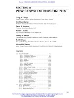
Figure 1.5 shows a simulation of an electron in free space traveling to the
right in the positive x direction. It is initialized at time T = 0. (See program
Se1_1.m in Appendix D .) After 1700 iterations, which represents a time of
FIGURE 1.5 A particle propagating in free space. The solid line represents the real
part of ψ and the dashed line represents the imaginary part.
5 10 15 20 25 30 35 40

−0.2
−0.1
0
0.1
0.2
0 fs
KE = 0.062 eV PE = 0.000 eV
Se1−1
5 10 15 20 25 30 35 40
−0.2
−0.1
0
0.1
0.2
34 fs
KE = 0.062 eV PE = 0.000 eV
5 10 15 20 25 30 35 40
−0.2
−0.1
0
0.1
0.2
68 fs
KE = 0.062 eV PE = 0.000 eV
nm