CALC GUIDE CHAPTER 3 CREATING CHARTS AND GRAPHS PRESENTING INFORMATION VISUALLY
Bạn đang xem bản rút gọn của tài liệu. Xem và tải ngay bản đầy đủ của tài liệu tại đây (1.67 MB, 42 trang )
Calc Guide
Chapter 3
Creating Charts and Graphs
Presenting information visually
Copyright
This document is Copyright © 2005–2013 by its contributors as listed below. You may distribute it
and/or modify it under the terms of either the GNU General Public License
( version 3 or later, or the Creative Commons Attribution
License ( version 3.0 or later.
All trademarks within this guide belong to their legitimate owners.
Contributors Christian Chenal Pierre-Yves Samyn
Laurent Balland-Poirier Shelagh Manton
Barbara Duprey Philippe Clément Peter Schofield
Jean Hollis Weber
John A Smith
Feedback
Please direct any comments or suggestions about this document to:
Acknowledgments
This chapter is based on Chapter 3 of the OpenOffice.org 3.3 Calc Guide. The contributors to that
chapter are:
Richard Barnes John Kane Peter Kupfer
Shelagh Manton Alexandre Martins Anthony Petrillo
Sowbhagya Sundaresan Jean Hollis Weber Linda Worthington
Ingrid Halama
Publication date and software version
Published 8 December 2013. Based on LibreOffice 4.1.
Note for Mac users
Some keystrokes and menu items are different on a Mac from those used in Windows and Linux.
The table below gives some common substitutions for the instructions in this chapter. For a more
detailed list, see the application Help.
Windows or Linux Mac equivalent Effect
Tools > Options LibreOffice > Preferences Access setup options
menu selection
Right-click Control+click or right-click Opens a context menu
depending on computer setup
Ctrl (Control) ⌘ (Command) Used with other keys
F5 Shift+⌘+F5 Opens the Navigator
F11 ⌘+T Opens the Styles and Formatting window
Documentation for LibreOffice is available at />
Contents
Copyright..............................................................................................................................2
Contributors................................................................................................................................. 2
Feedback..................................................................................................................................... 2
Acknowledgments........................................................................................................................ 2
Publication date and software version.........................................................................................2
Note for Mac users...............................................................................................................2
Introduction..........................................................................................................................5
Chart Wizard.........................................................................................................................5
Creating charts and graphs..........................................................................................................5
Selecting chart type..................................................................................................................... 7
Data range and axes labels.........................................................................................................7
Data series.................................................................................................................................. 8
Chart elements............................................................................................................................ 9
Editing charts and graphs.................................................................................................10
Changing chart type................................................................................................................... 10
Editing data ranges or data series..............................................................................................11
Basic editing of chart elements..................................................................................................11
Adding or removing chart elements............................................................................................11
Titles, subtitles and axes names............................................................................................11
Legends................................................................................................................................. 11
Axes...................................................................................................................................... 12
Grids..................................................................................................................................... 13
Data labels............................................................................................................................ 13
Trend lines............................................................................................................................ 15
Mean value lines................................................................................................................... 16
X or Y error bars.................................................................................................................... 16
Formatting charts and graphs..........................................................................................18
Selecting chart elements............................................................................................................ 18
Formatting options..................................................................................................................... 18
Moving chart elements............................................................................................................... 19
Changing chart area background...............................................................................................19
Changing chart graphic background..........................................................................................19
Changing colors......................................................................................................................... 20
3D charts................................................................................................................................... 20
Rotation and perspective.......................................................................................................21
Rotating 3D charts interactively.............................................................................................21
Appearance........................................................................................................................... 21
Illumination............................................................................................................................ 22
Grids.......................................................................................................................................... 23
Axes........................................................................................................................................... 23
Scale..................................................................................................................................... 24
Positioning............................................................................................................................. 25
Line....................................................................................................................................... 25
Label..................................................................................................................................... 25
Creating Charts and Graphs 3
Numbers............................................................................................................................... 26
Font and Font Effects............................................................................................................ 26
Asian Typography.................................................................................................................. 26
Hierarchical axis labels.............................................................................................................. 27
Selecting and formatting symbols..............................................................................................28
Adding drawing objects to charts....................................................................................28
Resizing and moving the chart.........................................................................................28
Interactively................................................................................................................................ 28
Position and Size dialog............................................................................................................. 29
Position and Size.................................................................................................................. 29
Rotation................................................................................................................................. 30
Slant & Corner Radius...........................................................................................................31
Exporting charts.................................................................................................................31
Gallery of chart types........................................................................................................31
Column charts............................................................................................................................ 31
Bar charts.................................................................................................................................. 32
Pie charts................................................................................................................................... 32
Area charts................................................................................................................................ 34
Line charts................................................................................................................................. 35
Scatter or XY charts................................................................................................................... 36
XY (Scatter)........................................................................................................................... 36
XY chart variants................................................................................................................... 36
Example of XY chart.............................................................................................................. 37
Bubble charts............................................................................................................................. 38
Net charts.................................................................................................................................. 39
Stock charts............................................................................................................................... 40
Stock chart variants............................................................................................................... 40
Setting data source............................................................................................................... 40
Organize data series............................................................................................................. 41
Setting data ranges............................................................................................................... 41
Legend.................................................................................................................................. 41
Column and line charts.............................................................................................................. 42
Creating Charts and Graphs 4
Introduction
Charts and graphs can be powerful ways to convey information to the reader. LibreOffice Calc
offers a variety of different chart and graph formats for your data.
Using Calc, you can customize charts and graphs to a considerable extent. Many of these options
enable you to present your information in the best and clearest manner.
For readers who are interested in effective ways to present information graphically, two excellent
introductions to the topic are William S. Cleveland’s The elements of graphing data, 2nd edition,
Hobart Press (1994) and Edward R. Tufte’s The Visual Display of Quantitative Information, 2nd
edition, Graphics Press (2001).
Chart Wizard
Calc uses a Chart Wizard to create charts or graphs from your spreadsheet data. After the chart
has been created as an object in your spreadsheet, you can then change the chart type, adjust
data ranges and the edit the chart using the functions available in the Chart Wizard. Each change
you make using is automatically reflected in the chart object placed onto your spreadsheet. This is
described in the following sections.
Creating charts and graphs
To demonstrate the process of creating charts and graphs in Calc, we will use example data as
shown in Figure 1 to create a chart.
Figure 1: Example data for creating a chart
1) Select the cells containing the data to be included in the chart by highlighting (Figure 1).
The selection does not need to be in a single block as in Figure 1; you can also choose
individual cells or groups of cells (columns or rows). See Chapter 1 Introducing Calc for
more information about selecting cells and ranges of cells.
2) Go to Insert > Chart on the main menu bar, or click the Chart icon on the Standard
toolbar to open the Chart Wizard dialog (Figure 2). A sample chart is created using the
selected data and is placed onto the spreadsheet as an object (Figure 3).
Chart Wizard 5
Figure 2: Chart Wizard dialog – selecting chart type
Figure 3: Example chart automatically created using Chart Wizard
Note If you want to plot any unconnected rows or columns of data, select the first data
series, then hold down the Ctrl key and select the next series. The two data series
you are selecting must be in separate columns or rows. Otherwise Calc will assume
that you are adding to the same data series.
Before opening the Chart Wizard, place the cursor or select a cell anywhere in the
Tip sample chart. Just be careful that you have not included the title of your chart when area of the data. The Chart Wizard will then guess the range of the data to create a
you make your selection.
Chart Wizard 6
Selecting chart type
Calc offers a choice of ten basic chart types and the options available vary according to the type of
chart you select.
The initial chart created using the Chart Wizard is a normal column chart and by default it is a 2D
chart. This is highlighted with a surrounding border in the preview box in Figure 2 and the chart
name is shown below the preview.
To change the chart type:
1) Select the type of chart from the list in Choose a chart type (Figure 2).
2) Select a chart icon in the preview box and check to see if it is the chart type you require.
For more information on chart types, see “Gallery of chart types” on page 31.
3) For Column, Bar, Pie or Area chart types only and if you want to use a 3D chart, select the
checkbox 3D Look and select the type of 3D view for your chart (Realistic or Simple).
4) Select the options you want to use for your chart. The options available are dependent of
the type of chart selected.
5) Click Next>> to move onto the next step in creating an example chart and make changes
to the data range and axes labels (Figure 4).
6) If you are satisfied with your chart, click Finish to close the Chart Wizard and create an
example chart object on your spreadsheet.
Note To demonstrate the process of creating charts using the following sections, please
leave the chart type as 2D column normal.
Figure 4: Chart Wizard dialog – selecting data range
Data range and axes labels
In the Data Range step of the Chart Wizard (Figure 4), you can manually correct any mistakes you
have made in selecting the data for your chart, how your chart is plotted and how to label your
chart.
1) If necessary, change the rows and columns used as data for your chart by editing the cell
references in the Data range text box.
Chart Wizard 7
2) Select whether to plot chart data by using either rows or columns as the data series. This is
useful if you use a chart type such as Donut or Pie to display your data.
3) Select whether to use the first row, or first column, or both, as labels for the axes of the
chart.
4) Click Next>> to move onto the next step in creating an example chart and make changes
to the data series (Figure 5).
5) If you are satisfied with your chart, click Finish to close the Chart Wizard and create an
example chart object on your spreadsheet.
Note A data range may consist of more than one region in a spreadsheet, for example
"$Sheet1.A1:A5;$Sheet1.D1:D5" is also a valid data range.
If you want a data range of multiple cell areas that are not next to each other, enter
the first range, then manually add a semicolon at the end of the text box, then enter
the other ranges. Use a semicolon as delimiter between ranges.
Figure 5: Chart Wizard dialog – selecting data series
Data series
On the Data Series page of the Chart Wizard (Figure 5) you can change the source range of all
data series separately, including their labels. You can also change the range of the categories and
remove unnecessary data series or add data series from other cells.
Each named data series has its ranges and its individual Y-values listed. This is useful if you have
very specific requirements for data in your chart, as you can include or leave out these ranges.
In the Data series list box you see a list of all data series in the current chart.
1) To organize the data series, select an entry in the Data series list.
2) Click Add to add another data series below the selected entry. The new data series has the
same type as the selected entry.
3) Click Remove to remove the selected entry from the Data series list.
4) Use the Up and Down buttons to move the selected entry in the list up or down. This does
not change the order in the data source table, but changes only the arrangement in the
chart.
Chart Wizard 8
5) To change the cell reference that is used to name a data series, select an entry in the Data
series list and edit the cell reference in the Range for Name text box.
6) To change the cell reference that is to give a category in a data series, select an entry in
the Data series list and edit the cell reference in the Categories text box.
7) Click Next>> to move onto the next step in creating an example chart and make changes
to the chart elements (Figure 7).
8) If you are satisfied with your chart, click Finish to close the Chart Wizard and create an
example chart object on your spreadsheet.
Figure 6: Chart elements
Chart elements
The chart elements for 2D and 3D charts are shown in Figure 6.
• The chart wall contains the graphic of the chart displaying the data.
• The chart area is the area surrounding the chart graphic.
• The chart floor is only available for 3D charts.
• The chart title and subtitle, chart legend, axes labels and axes names are in the chart area
and can be added when using the Chart Wizard to create a chart.
On the Chart Elements page (Figure 7), you can add or change the titles, axes names and grids.
Use a title that draws the attention of viewers to the purpose of the chart and what you want them
to see. Figure 6 shows the various chart elements that can be placed onto a chart.
1) Enter a title and subtitle you want to use in the Title and Subtitle text boxes. For example,
a better title for this example chart might be The Performance of Motor and Other Rental
Boats.
2) Enter a name you want to use in the X axis and Y axis text boxes, for example,
Thousands for the Y axis. The Z axis text box is only active if you are creating a 3D chart.
3) Select the Display legend checkbox and where you want the legend displayed on your
chart – Left, Right, Top or Bottom.
4) In Display grids, select the X axis or Y axis checkboxes to display a grid on your chart. The
Z axis checkbox is only active if you are creating a 3D chart. Grid lines are not available for
pie charts.
Chart Wizard 9
5) Click Finish to close the Chart Wizard and create an example chart object on your
spreadsheet.
Figure 7: Chart Wizard dialog – selecting and changing chart elements
Note Clicking Finish closes the Chart Wizard, but the chart is still in edit mode and you
can still modify it. Click outside the chart in any cell or a data series to complete the
chart creation.
Editing charts and graphs
After you have created a chart, you may find that data has changed or you would like to improve
the look of the chart. Calc provides tools for changing the chart type, chart elements, data ranges,
fonts, colors, and many other options, and this is described in the following sections.
Changing chart type
You can change the chart type at any time.
1) Select the chart by double-clicking on it to enter edit mode. The chart should now be
surrounded by a gray border.
2) Go to Format > Chart Type on the main menu bar, or click the Chart Type icon on the
Formatting toolbar, or right-click on the chart and select Chart Type from the context menu
to open the Chart Type dialog. This is similar to the Chart Wizard dialog shown in Figure 2
on page 7.
3) Select a replacement chart type you want to use. For more information, see “Selecting
chart type” on page 7.
4) Click OK to close the dialog.
5) Click outside the chart to leave edit mode.
Editing charts and graphs 10
Editing data ranges or data series
If the data range or data series has changed in your spreadsheet, you can edit them in your chart.
1) Select the chart by double-clicking on it to enter edit mode. The chart should now be
surrounded by a gray border.
2) Go to Format > Data Ranges on the main menu bar, or right-click on the chart and select
Data Ranges from the context menu to open the Data Ranges dialog. This dialog has
similar pages to the Chart Wizard dialogs shown in Figure 4 on page 7 and Figure 5 on
page 8.
3) To edit the data range used for the chart, click on the Data Range tab. For more
information, see “Data range and axes labels” on page 7.
4) To edit the data series used for the chart, click on the Data Series tab. For more
information, see “Data series” on page 8.
5) Click OK to close the dialog.
6) Click outside the chart to leave edit mode.
Basic editing of chart elements
Basic editing of the title, subtitle and axes names in your chart is as follows. For more advanced
editing, see the following sections.
1) Select the chart by double-clicking on it to enter edit mode. The chart should now be
surrounded by a gray border.
2) Go to Insert > Titles on the main menu bar, or right-click in the chart area and select Insert
Titles from the context menu to open the Titles dialog. This dialog is similar to the Chart
Wizard dialog shown in Figure 7 on page 10.
3) Edit the text shown in the various text boxes.
4) Click OK to close the dialog.
5) Click outside the chart to leave edit mode.
Adding or removing chart elements
Titles, subtitles and axes names
Adding a title, subtitle or axes names to your chart is the same procedure as given in “Basic editing
of chart elements” above. To remove a title, subtitle or axes names from your chart:
1) Select the chart by double-clicking on it to enter edit mode. The chart should now be
surrounded by a gray border.
2) Open the Titles dialog as above and delete the text from the various text boxes.
3) Click OK to close the dialog.
4) Click outside the chart to leave edit mode.
Legends
To add a legend to your chart:
1) Select the chart by double-clicking on it to enter edit mode. The chart should now be
surrounded by a gray border.
2) Go to Insert > Legend on the main menu bar to open the Legend dialog. This dialog is
similar to the Display legend section on the Chart Wizard dialog shown in Figure 7 on
page 10.
3) Select the Display legend checkbox and where you want the legend displayed on your
chart – Left, Right, Top or Bottom.
Editing charts and graphs 11
4) Click OK to close the dialog.
5) Alternatively, right-click in the chart area and select Insert Legend from the context menu
to insert a legend in the default position on the right side of the chart.
6) Click outside the chart to leave edit mode.
To remove a legend from your chart:
1) Select the chart by double-clicking on it to enter edit mode. The chart should now be
surrounded by a gray border.
2) Go to Insert > Legend on the main menu bar to open the Legend dialog.
3) Deselect the Display legend checkbox.
4) Click OK to close the dialog.
5) Alternatively, right-click in the chart area and select Delete Legend from the context menu.
6) Click outside the chart to leave edit mode.
Axes
To add an axis to your chart:
1) Select the chart by double-clicking on it to enter edit mode. The chart should now be
surrounded by a gray border.
2) Go to Insert > Axes on the main menu bar, or right-click on the chart and select
Insert/Delete Axes from the context menu to open the Axes dialog (Figure 8).
3) Select the axes checkboxes that you want to use on your chart. The Z axis checkbox is
only active if you are creating a 3D chart.
4) Click OK to close the dialog.
5) Click outside the chart to leave edit mode.
To remove an axis from your chart:
1) Select the chart by double-clicking on it to enter edit mode. The chart should now be
surrounded by a gray border.
2) Open the Axes dialog as above and deselect the checkboxes for the axes you want to
remove.
3) Click OK to close the dialog.
4) Click outside the chart to leave edit mode.
Figure 8: Axes dialog
Grids
The visible grid lines can help to estimate the data values in the chart. The distance of the grid
lines corresponds to the interval settings in the Scale tab of the axis properties.
Editing charts and graphs 12
Grid lines are not available for pie charts.
To add a grid to your chart:
1) Select the chart by double-clicking on it to enter edit mode. The chart should now be
surrounded by a gray border.
2) Go to Insert > Grids on the main menu bar to open the Grids dialog. This is the same
dialog as the Axes dialog (Figure 8), but it is titled Grids.
3) Select the grid checkboxes that you want to use on your chart. The Z axis checkbox is only
active if you are creating a 3D chart.
4) Click OK to close the dialog.
5) Click outside the chart to leave edit mode.
To remove a grid from your chart:
1) Select the chart by double-clicking on it to enter edit mode. The chart should now be
surrounded by a gray border.
2) Open the Grids dialog as above and deselect the checkboxes for the grids you want to
remove.
3) Click OK to close the dialog.
4) Click outside the chart to leave edit mode.
Data labels
Data labels put information about each data point on the chart. They can be very useful for
presenting detailed information, but you need to be careful not to create a chart that is too cluttered
to read.
Figure 9: Data Labels dialog
Note The text for data labels is taken from the spreadsheet data and it cannot be changed
here. If the text needs to be abbreviated, or if it did not label your graph as you were
expecting, you need to change it in the original data table.
To add data labels to your chart:
1) Select the chart by double-clicking on it to enter edit mode. The chart should now be
surrounded by a gray border.
Editing charts and graphs 13
2) Select the data series on your chart that you want to label. If you do not select a data
series, then all data series on your chart will be labelled.
3) Go to Insert > Data Labels on the menu bar to open the Data Labels dialog (Figure 9).
4) Select the options that you want to use for data labels. The options available for data labels
are explained below.
5) Click OK to close the dialog.
6) Alternatively, right-click on the selected data series and select Insert Data Labels from the
context menu. This method uses the default setting for the data labels.
7) Click outside the chart to leave edit mode.
To remove data labels from you chart:
1) Select the chart by double-clicking on it to enter edit mode. The chart should now be
surrounded by a gray border.
2) Select the data labels on your chart that you want to remove.
3) Go to Insert > Data Labels on the menu bar, or right-click on the data labels and select
Format Data Labels from the context menu to open the Data Labels dialog (Figure 9).
4) Make sure Data Labels page is selected in the dialog and deselect all the options for the
data labels that you want to remove.
5) Click OK to close the dialog and remove the data labels.
6) Alternatively, right-click on the data series and select Delete Data Labels from the context
menu.
7) Repeat the above steps to remove more data labels because you can only remove one
data series at a time.
8) Click outside the chart to leave edit mode.
The options available for data labels in the Data Labels dialog are as follows.
• Show value as number – displays the numeric values of the data points. When selected,
this option activates the Number format button.
• Number format – opens the Number Format dialog, where you can select the number
format. This dialog is very similar to the one for formatting numbers in cells, see Chapter 2
Entering, Editing, and Formatting Data for more information.
• Show value as percentage – displays the percentage value of the data points in each
column. When selected, this option activates the Percentage format button.
• Percentage format – opens the Number Format dialog, where you can select the
percentage format. This dialog is very similar to the one for formatting numbers in cells, see
Chapter 2 Entering, Editing, and Formatting Data for more information.
• Show category – shows the data point text labels.
• Show legend key – displays the legend icons next to each data point label.
• Separator – selects the separator between multiple text strings for the same object (if at
least two options above are selected).
• Placement – selects the placement of data labels relative to the objects.
• Rotate Text – click in the dial to set the text orientation for the data labels or enter the
rotation angle for the data labels.
• Text Direction – specify the text direction for a paragraph that uses Complex Text Layout
(CTL). This feature is only available if CTL support is enabled.
Trend lines
When you have a scattered grouping of points in a graph, you may want to show the relationship of
the points by using a trend line. Calc has a good selection of regression types you can use for
Editing charts and graphs 14
trend lines: linear, logarithm, exponential, and power. Choose the type that comes closest to
passing through all of the points.
Trend lines can be added to all 2D chart types except for pie and stock charts. If a data series is
selected, a trend line is inserted for that data series only. If no data series are selected, trend lines
are inserted for all data series.
When inserted, trend lines are automatically shown in the chart legend.
Figure 10: Trend Lines dialog
To insert trend lines to your chart:
1) Select the chart by double-clicking on it to enter edit mode. The chart should now be
surrounded by a gray border.
2) Select the data series on your chart that you want to use to insert trend lines. If you do not
select a data series, then trend lines for all data series on your chart will be inserted.
3) To insert trend lines for all data series, go to Insert > Trend Lines on the main menu bar to
open the Trend Lines dialog (Figure 10).
4) To insert a trend line for a single data series, select a data series then go to Insert > Trend
Lines on the main menu bar, or right-click on the data series and select Insert Trend Line
from the context menu to open the Trend Lines dialog for the selected data series.
Note The dialog to insert a trend line for a single data series is similar to the dialog for all
data series (Figure 10), but has a second page called Line where you can select the
formatting for the trend line (style, color, width, and transparency).
5) Select the type of trend line that you want to insert – Linear, Logarithmic, Exponential, or
Power.
6) To show the equation or coefficient of determination used to calculate the trend lines, select
the options Show equation and/or Show coefficient of determination (R2).
7) Click OK to close the dialog and the trend lines are placed onto your chart.
8) Click outside the chart to leave edit mode.
Editing charts and graphs 15
Note When inserted, a trend line has the same color as the corresponding data series. To
change the trend line properties, right-click on the trend line and select Format
Trend Line on the context menu to open the Line page of the Trend Lines dialog.
To show the equation or the coefficient of determination and the equation after a trend line has
been inserted, right-click on the trend line and select Insert Trend Line Equation or Insert R2 and
Trend Line Equation from the context menu. For more information on the equations, see the topic
Trend Lines in the LibreOffice Calc Help.
When you select a trend line, the information for the trend line is shown in the Status Bar, which is
normally located at the bottom of the spreadsheet.
To delete trend lines from your chart:
1) Select the chart by double-clicking on it to enter edit mode. The chart should now be
surrounded by a gray border.
2) To delete all trend lines, go to Insert > Trend Lines on the main menu bar to open the
Trend Lines dialog and select None then click OK.
3) To delete a single trend line, right-click on the data series and select Delete Trend line
from the context menu.
Mean value lines
Mean value lines are special trend lines that show the mean value and can only be used in 2D
charts. If a data series is selected, a mean value line is inserted for that data series only. If no data
series are selected, mean value lines are inserted for all data series.
When you insert mean value lines into your chart, Calc calculates the average of each selected
data series and places a colored line at the correct level in the chart. The colored line uses the
same color as that used for the data series.
To insert mean value lines on your chart:
1) Select the chart by double-clicking on it to enter edit mode. The chart should now be
surrounded by a gray border.
2) Select the data series on your chart that you want to use to insert mean value lines. If you
do not select a data series, then mean value lines for all data series on your chart will be
inserted.
3) To insert mean value lines for all data series, go to Insert > Mean Value Lines on the main
menu bar.
4) To insert a mean value line for a single data series, select a data series then go to Insert >
Mean Value Lines on the main menu bar, or right-click on the data series and select Insert
Mean Value Line from the context menu.
5) Click outside the chart to leave edit mode.
To delete mean value lines from your chart:
1) Select the chart by double-clicking on it to enter edit mode. The chart should now be
surrounded by a gray border.
2) Select the mean value line you want to delete and press the Delete key, or right-click on the
data series and select Delete Mean Value Line from the context menu.
3) Click outside the chart to leave edit mode.
X or Y error bars
Use the X and Y error bars to display error bars for 2D charts only. If a data series is selected, an X
or Y error bar is inserted for that data series only. If no data series are selected, X or Y error bars
are inserted for all data series.
Editing charts and graphs 16
If you are presenting data that has a known possibility of error, such as social surveys using a
particular sampling method, or you want to show the measuring accuracy of the tool you used, you
may want to show error bars on the chart.
To insert error bars to your chart:
1) Select the chart by double-clicking on it to enter edit mode. The chart should now be
surrounded by a gray border.
Figure 11: Error Bars dialog
2) Select the data series on your chart that you want to use to insert error bars. If you do not
select a data series, then error bars for all data series on your chart will be inserted.
3) To insert error bars for all data series, go to Insert > X Error Bars or Insert > Y Error Bars
on the main menu bar to open the Error Bars dialog (Figure 11).
4) To insert error bars for a single data series, select a data series then go to Insert > X Error
Bars or Insert > Y Error Bars on the main menu bar, or right-click on the data series and
select Insert X Error Bars or Insert Y Error Bars from the context menu to open the Error
Bars dialog.
5) Select the required options in Error Category, Error Indicator or Parameters to use for the
error bars. More information on the options for error bars is given below.
6) Click OK to close the dialog and insert the error bars onto your chart.
7) Click outside the chart to leave edit mode.
To delete error bars from your chart:
1) Select the chart by double-clicking on it to enter edit mode. The chart should now be
surrounded by a gray border.
2) To delete error bars for all data series, go to Insert > X Error Bars or Insert > Y Error
Bars on the main menu bar to open the Error Bars dialog (Figure 11) and select None in
Error Category.
3) Click OK to close the dialog and delete the error bars from your chart.
4) To delete error bars from a single data series, right-click on the data series and select
Delete X Error Bars or Delete Y Error Bars from the context menu.
5) Click outside the chart to leave edit mode.
Several options are provided on the X or Y Error Bars dialog. You can select only one error
category at a time. You can also select whether the error indicator shows both positive and
negative errors, or only positive or only negative.
Editing charts and graphs 17
• Constant value – you can have separate positive and negative values.
• Percentage – choose the error as a percentage of the data points.
• The drop-down list has four options as follows:
– Standard error
– Variance – shows error calculated on variance
– Standard deviation – shows error calculated on standard deviation
– Error margin – you designate the error
• Cell Range – calculates the error based on cell ranges you select. The Parameters section
at the bottom of the dialog changes to allow selection of the cell ranges.
Formatting charts and graphs
Calc provides many options for formatting and fine-tuning the appearance of your charts. To enter
formatting mode for your chart:
Selecting chart elements
Depending on the purpose of your document, for example a screen presentation or a printed
document for a black and white publication, you might wish to have more detailed control over the
different chart elements to give you what you need.
To select a chart element:
1) Select the chart by double-clicking on it to enter edit mode. The chart should now be
surrounded by a gray border.
2) Select the chart element that you want to format and the chart element will be highlighted
with selection squares or a border of square selection handles. Each chart element has its
own formatting options and these are explained below.
3) Go to Format on the main menu bar and select the relevant option, or right-click to display
a context menu relevant to the selected element to open the relevant formatting dialog.
Note If your chart has many elements, it is recommended to turn on tooltips in Tools >
Options > LibreOffice > General. When you hover a cursor over an element, Calc
will display the element name which will making it easier in selecting the correct
element. The name of the selected element also appears in the Status Bar.
Formatting options
• Format Selection – opens a dialog where you can specify the area fill, borders,
transparency, characters, fonts, and other attributes of the selected element on the chart.
• Position and Size – opens the Position and Size dialog (see “Position and Size dialog” on
page 29).
• Arrangement – provides two options: Bring Forward and Send Backward, of which only
one may be active for some items. Use these options to arrange overlapping data series.
• Title – formats the titles for the chart and chart axes.
• Legend – formats how the legend appears and positioned on the chart
• Axis – formats the lines that create the chart as well as the font of the text that appears on
both the X and Y axes.
Formatting charts and graphs 18
• Grid – formats the lines that create a grid for the chart.
• Chart Wall, Chart Floor, or Chart Area – formats how the chart wall, chart floor and chart
area appear on your chart. Note that the chart floor is available for 3D charts.
• Chart Type – changes what type of chart is displayed and whether it is 2D or 3D chart.
Note that only column, bar, pie and area charts can be displayed as a 3D chart.
• Data Ranges – explained in “Data range and axes labels” on page 7 and “Editing data
ranges or data series” on page 11.
• 3D View – formats 3D charts and is only available for 3D charts (see page 20).
Moving chart elements
You may wish to move or resize individual elements of a chart, independent of other chart
elements. For example, you may wish to reposition the legend from its default position on the right
of the chart to below the chart. Pie charts also allow moving of individual wedges of the pie as well
as exploding the entire pie. However, you cannot move an individual point or data series.
1) Select the chart by double-clicking on it to enter edit mode. The chart should now be
surrounded by a gray border.
2) Move the cursor over the chart element you want to move, then click and drag to move the
element. If the element is already selected, then the cursor changes to the move icon
(normally a small hand), then click and drag to move the element.
3) Release the mouse button when the element is in the desired position.
Note If your chart is a 3D chart, then round selection handles appear when a 3D chart
element is selected. These round selection handles control the 3D angle of the
element. You cannot resize or reposition the element while the round selection
handles are showing. Use Shift+Click to get the square selection handles and you
can now resize and reposition your 3D chart graphic.
Changing chart area background
The chart area is the area surrounding the chart graphic, including the main title, subtitle and
legend.
1) Select the chart by double-clicking on it to enter edit mode. The chart should now be
surrounded by a gray border.
2) Go to Format > Chart Area on the main menu bar or right-click in the chart area and select
Format Chart Area from the context menu to open the Chart Area dialog (Figure 12).
3) Select the desired formatting from the Borders, Area and Transparency pages.
4) Click OK to close the dialog and save your changes.
Changing chart graphic background
The Chart Wall is the area that contains the chart graphic.
1) Select the chart by double-clicking on it to enter edit mode. The chart should now be
surrounded by a gray border.
2) Go to Format > Chart Wall on the main menu bar or right-click in the chart area and select
Format Chart Area from the context menu to open the Chart Wall dialog. This dialog is
similar to the Chart Area dialog in Figure 12.
3) Select the desired formatting from the Borders, Area and Transparency pages.
4) Click OK to close the dialog and save your changes.
Formatting charts and graphs 19
Figure 12: Chart Area dialog
Changing colors
If you want to modify the color scheme from the default, or you want to add extra chart colors for
charts in all your documents, go to Tools > Options > Charts > Default Colors top make the
changes. Changes made in this dialog affect the default chart colors for any chart you make in the
future. See the Getting Started Guide for more information on changing colors.
3D charts
The 3D View dialog (Figure 13) has three pages:
• Perspective – where you can change the perspective of the chart.
• Appearance – Select whether to use a simple or realistic scheme for your 3D chart.
• Illumination – controls the light source that illuminates your 3D chart and where the
shadows will fall.
Figure 13: 3D View dialog – Perspective page
Formatting charts and graphs 20