Elliptic Functions, by Arthur L. Baker doc
Bạn đang xem bản rút gọn của tài liệu. Xem và tải ngay bản đầy đủ của tài liệu tại đây (583.56 KB, 147 trang )
The Project Gutenberg EBook of Elliptic Functions, by Arthur L. Baker
This eBook is for the use of anyone anywhere at no cost and with
almost no restrictions whatsoever. You may copy it, give it away or
re-use it under the terms of the Project Gutenberg License included
with this eBook or online at www.gutenberg.org
Title: Elliptic Functions
An Elementary Text-Book for Students of Mathematics
Author: Arthur L. Baker
Release Date: January 25, 2010 [EBook #31076]
Language: English
Character set encoding: ISO-8859-1
*** START OF THIS PROJECT GUTENBERG EBOOK ELLIPTIC FUNCTIONS ***
Produced by Andrew D. Hwang, Brenda Lewis and the Online
Distributed Proofreading Team at (This
file was produced from images from the Cornell University
Library: Historical Mathematics Monographs collection.)
transcriber’s note
This book was produced from images provided by the Cornell
University Library: Historical Mathematics Monographs
collection.
Minor typographical corrections and presentational changes have
been made without comment. The calculations preceding
equation (15) on page 12 (page 12 of the original) have been
re-formatted.
This PDF file is optimized for screen viewing, but may
easily be recompiled for printing. Please see the preamble
of the L
A
T
E
X source file for instructions.
Elliptic Functions.
An Elementary Text-Book for
Students of Mathematics.
BY
ARTHUR L. BAKER, C.E., Ph.D.,
Professor of Mathematics in the Stevens School of the Stevens Institute of
Technology, Hoboken, N. J.; formerly Professor in the Pardee
Scientific Department, Lafayette College, Easton, Pa.
sin am u =
1
√
k
·
H(u)
Θ(u)
.
NEW YORK:
J O H N W I L E Y & S O N S,
53 East Tenth Street.
1890.
Copyright, 1890,
BY
Arthur L. Baker.
Robert Drummond,
Electrotyper,
444 & 446 Pearl Street,
New York.
Ferris Bros.,
Printers,
326 Pearl Street,
New York.
PREFACE.
In the works of Abel, Euler, Jacobi, Legendre, and others, the stu-
dent of Mathematics has a most abundant supply of material for the
study of the subject of Elliptic Functions.
These works, however, are not accessible to the general student, and,
in addition to being very technical in their treatment of the subject, are
moreover in a foreign language.
It is in the hope of smoothing the road to this interesting and increas-
ingly important branch of Mathematics, and of putting within reach of
the English student a tolerably complete outline of the subject, clothed
in simple mathematical language and methods, that the present work
has been compiled.
New or original methods of treatment are not to be looked for. The
most that can be expected will be the simplifying of methods and the
reduction of them to such as will be intelligible to the average student
of Higher Mathematics.
I have endeavored throughout to use only such methods as are fa-
miliar to the ordinary student of Calculus, avoiding those methods of
discussion dependent upon the properties of double periodicity, and
also those depending upon Functions of Complex Variables. For the
same reason I have not carried the discussion of the Θ and H functions
further.
Among the minor helps to simplicity is the use of zero subscripts to
indicate decreasing series in the Landen Transformation, and of numer-
ical subscripts to indicate increasing series. I have adopted the notation
of Gudermann, as being more simple than that of Jacobi.
I have made free use of the following works: Jacobi’s Fun-
damenta Nova Theoriæ Func. Ellip.; Houel’s Calcul Infinit
´
esimal;
Legendre’s Trait
´
e des Fonctions Elliptiques; Durege’s Theorie der
Elliptischen Functionen; Hermite’s Th
´
eorie des Fonctions Ellip-
tiques; Verhulst’s Th
´
eorie des Functions Elliptiques; Bertrand’s
Calcul Int
´
egral; Laurent’s Th
´
eorie des Fonctions Elliptiques; Cay-
ley’s Elliptic Functions; Byerly’s Integral Calculus; Schlomilch’s
Die H
¨
oheren Analysis; Briot et Bouquet’s Fonctions Elliptiques.
I have refrained from any reference to the Gudermann or Weier-
strass functions as not within the scope of this work, though the Gu-
dermannians might have been interesting examples of verification for-
mulæ. The arithmetico-geometrical mean, the march of the functions,
and other interesting investigations have been left out for want of room.
CONTENTS
pageIntroductory Chapter. . . . . . . . 1
Chap. I. Elliptic Integrals. . . . . . . 4
II. Elliptic Functions. . . . . . . 16
III. Periodicity of the Functions. . . . . 24
IV. Landen’s Transformation . . . . . 33
V. Complete Functions . . . . . . 50
VI. Evaluation for φ. . . . . . . 53
VII. Development of Elliptic Functions into Factors. . 56
VIII. The Θ Function. . . . . . . . 71
IX. The Θ and H Functions. . . . . . 74
X. Elliptic Integrals of the Second Order. . . . 86
XI. Elliptic Integrals of the Third Order. . . . 96
XII. Numerical Calculations. q. . . . . . 101
XIII. Numerical Calculations. K . . . . . . 105
XIV. Numerical Calculations. u . . . . . 111
XV. Numerical Calculations. φ. . . . . . 119
XVI. Numerical Calculations. E(k, φ). . . . . 123
XVII. Applications. . . . . . . . 128
ELLIPTIC FUNCTIONS.
INTRODUCTORY CHAPTER.
∗
The first step taken in the theory of Elliptic Functions was the de-
termination of a relation between the amplitudes of three functions of
either order, such that there should exist an algebraic relation between
the three functions themselves of which these were the amplitudes. It
is one of the most remarkable discoveries which science owes to Euler.
In 1761 he gave to the world the complete integration of an equation
of two terms, each an elliptic function of the first or second order, not
separately integrable.
This integration introduced an arbitrary constant in the form of a
third function, related to the first two by a given equation between the
amplitudes of the three.
In 1775 Landen, an English mathematician, published his celebrated
theorem showing that any arc of a hyperbola may be measured by two
arcs of an ellipse, an important element of the theory of Elliptic Func-
tions, but then an isolated result. The great problem of comparison of
Elliptic Functions of different moduli remained unsolved, though Euler,
in a measure, exhausted the comparison of functions of the same mod-
ulus. It was completed in 1784 by Lagrange, and for the computation
of numerical results leaves little to be desired. The value of a function
may be determined by it, in terms of increasing or diminishing moduli,
∗
Condensed from an article by Rev. Henry Moseley, M.A., F.R.S., Prof. of Nat. Phil.
and Ast., King’s College, London.
ELLIPTIC FUNCTIONS. 2
until at length it depends upon a function having a modulus of zero, or
unity.
For all practical purposes this was sufficient. The enormous task
of calculating tables was undertaken by Legendre. His labors did not
end here, however. There is none of the discoveries of his predecessors
which has not received some perfection at his hands; and it was he who
first supplied to the whole that connection and arrangement which have
made it an independent science.
The theory of Elliptic Integrals remained at a standstill from 1786,
the year when Legendre took it up, until the year 1827, when the sec-
ond volume of his Trait
´
e des Fonctions Elliptiques appeared. Scarcely
so, however, when there appeared the researches of Jacobi, a Professor
of Mathematics in K
¨
onigsberg, in the 123d number of the Journal of
Schumacher, and those of Abel, Professor of Mathematics at Christia-
nia, in the 3d number of Crelle’s Journal for 1827.
These publications put the theory of Elliptic Functions upon an en-
tirely new basis. The researches of Jacobi have for their principal object
the development of that general relation of functions of the first order
having different moduli, of which the scales of Lagrange and Legendre
are particular cases.
It was to Abel that the idea first occurred of treating the Elliptic In-
tegral as a function of its amplitude. Proceeding from this new point
of view, he embraced in his speculations all the principal results of Ja-
cobi. Having undertaken to develop the principle upon which rests the
fundamental proposition of Euler establishing an algebraic relation be-
tween three functions which have the same moduli, dependent upon
a certain relation of their amplitudes, he has extended it from three to
an indefinite number of functions; and from Elliptic Functions to an
infinite number of other functions embraced under an indefinite num-
ber of classes, of which that of Elliptic Functions is but one; and each
class having a division analogous to that of Elliptic Functions into three
INTRODUCTORY CHAPTER.
∗
3
orders having common properties.
The discovery of Abel is of infinite moment as presenting the first
step of approach towards a more complete theory of the infinite class
of ultra elliptic functions, destined probably ere long to constitute one
of the most important of the branches of transcendental analysis, and
to include among the integrals of which it effects the solution some of
those which at present arrest the researches of the philosopher in the
very elements of physics.
CHAPTER I.
ELLIPTIC INTEGRALS.
The integration of irrational expressions of the form
X dx
A + Bx + Cx
2
,
or
X dx
√
A + Bx + Cx
2
,
X being a rational function of x, is fully illustrated in most elemen-
tary works on Integral Calculus, and shown to depend upon the tran-
scendentals known as logarithms and circular functions, which can be
calculated by the proper logarithmic and trigonometric tables.
When, however, we undertake to integrate irrational expressions
containing higher powers of x than the square, we meet with insur-
mountable difficulties. This arises from the fact that the integral sought
depends upon a new set of transcendentals, to which has been given
the name of elliptic functions, and whose characteristics we will learn
hereafter.
The name of Elliptic Integrals has been given to the simple integral
forms to which can be reduced all integrals of the form
(1) V =
F(X, R ) dx,
where F(X, R) designates a rational function of x and R, and R repre-
sents a radical of the form
R =
Ax
4
+ Bx
3
+ Cx
2
+ Dx + E,
ELLIPTIC INTEGRALS. 5
where A, B, C, D, E indicate constant coefficients.
We will show presently that all cases of Eq. (1) can be reduced to
the three typical forms
(2)
x
0
dx
(1 − x
2
)(1 − k
2
x
2
)
,
x
0
x
2
dx
(1 − x
2
)(1 − k
2
x
2
)
,
x
0
dx
(x
2
+ a)
(1 − x
2
)(1 − k
2
x
2
)
,
which are called elliptic integrals of the first, second, and third order.
Why they are called Elliptic Integrals we will learn further on. The
transcendental functions which depend upon these integrals, and which
will be discussed in Chapter IV, are called Elliptic Functions.
The most general form of Eq. (1) is
(3) V =
A + BR
C + DR
dx;
where A, B, C, and D stand for rational integral functions of x.
A + BR
C + DR
can be written
A + BR
C + DR
=
AC − BDR
2
C
2
− D
2
R
2
−
(AD −CB)R
2
C
2
− D
2
R
2
·
1
R
= N −
P
R
;
N and P being rational integral functions of x. Whence Eq. (3) becomes
(4) V =
N dx −
P dx
R
.
ELLIPTIC FUNCTIONS. 6
Eq. (4) shows that the most general form of V can be made to de-
pend upon the expressions
(5) V
=
P dx
R
,
and
N dx.
This last form is rational, and needs no discussion here.
We can write
P =
G
0
+ G
1
x + G
2
x
2
+ ···
H
0
+ H
1
x + H
2
x
2
+ ···
=
G
0
+ G
2
x
2
+ G
4
x
4
+ ··· + (G
1
+ G
3
x
2
+ ···)x
H
0
+ H
2
x
2
+ H
4
x
4
+ ··· + (H
1
+ H
3
x
2
+ ···)x
.
Multiplying both numerator and denominator by
H
0
+ H
2
x
2
+ H
4
x
4
+ ··· −(H
1
+ H
3
x
2
+ H
5
x
4
+ ···)x,
we have a new denominator which contains only powers of x
2
. The
result takes the following form:
P =
M
0
+ M
2
x
2
+ M
4
x
4
+ ··· + (M
1
+ M
3
x
2
+ M
5
x
4
+ ···)x
N
0
+ N
2
x
2
+ N
4
x
4
+ N
6
x
6
+ ···
= Φ(x
2
) + Ψ(x
2
) · x.
Equation ( 5) thus becomes
(6) V
=
Φ(x
2
) dx
R
+
Ψ(x
2
) · x ·dx
R
.
We shall see presently that R can always be assumed to be of the
form
(1 − x
2
)(1 − k
2
x
2
).
ELLIPTIC INTEGRALS. 7
Therefore, putting x
2
= z, the second integral in Eq. (6) takes the
form
1
2
Ψ(z) · dz
(1 − z)(1 −k
2
z)
,
which can be integrated by the well-known methods of Integral Calcu-
lus, resulting in logarithmic and circular transcendentals.
There remains, therefore, only the form
Φ(x
2
) dx
R
to be determined.
We will now show that R can always be assumed to be in the form
(1 − x
2
)(1 − k
2
x
2
).
We have
R =
Ax
4
+ Bx
3
+ Cx
2
+ Dx + E
=
G(x −a)(x −b)(x −c)(x −d ),
a, b, c, and d being the roots of the polynomial of the fourth degree, and
G any number, real or imaginary, depending upon the coefficients in
the given polynomial.
Substituting in equation ( 1)
x =
p + qy
1 + y
,
we have
V =
φ(y , ρ) dy,(7)
ELLIPTIC FUNCTIONS. 8
ρ designating the radical
ρ =
G[p −a + (q − a)y][p − b + (q −b)y][p − c + (q −c)y] ··· .
In order that the odd powers of y under the radical may disappear
we must have their coefficients equal to zero; i.e.,
(p −a)(q −b) + (p − b)(q − a) = 0,
(p −c)(q − d) + (p −d)(q −c) = 0;
whence
2pq −(p + q)(a + b) + 2ab = 0,
2pq −(p + q)(c + d) + 2cd = 0,
and
(8)
pq =
ab(c + d) −cd(a + b)
a + b − (c + d)
,
p + q =
2ab −2cd
a + b − (c + d)
.
Equation (8) shows that p and q are real quantities, whether the roots
a, b, c, and d are real or imaginary; a, b, and c, d being the conjugate
pairs.
Hence equation (1) can always be reduced to the form of equa-
tion (7), which contains only the second and fourth powers of the vari-
able.
This transformation seems to fail when a + b −(c + d) = 0; but in that
case we have
R =
G[x
2
−(a + b)x + ab][x
2
−(a + b)x + cd],
ELLIPTIC INTEGRALS. 9
and substituting
x = y −
a + b
2
will cause the odd powers of y to disappear as before.
If the radical should have the form
G(x −a)(x −b)(x −c),
placing x = y
2
+ a, we get
V =
φ(y , ρ) dy,
ρ =
G(y
2
+ a − b)(y
2
+ a − c),
φ designating a rational function of y and ρ.
Thus all integrals of the form contained in equation (1), in which
R stands for a quadratic surd of the third or fourth degree, can be
reduced to the form
(9) V =
φ(x, R) dx,
R designating a radical of the form
G(1 + mx
2
)(1 + nx
2
),
m and n designating constants.
It is evident that if we put
x
= x
√
−m, k
2
= −
n
m
,
we can reduce the radical to the form
(1 − x
2
)(1 − k
2
x
2
).
ELLIPTIC FUNCTIONS. 10
We shall see later on that the quantity k
2
, to which has been given
the name modulus, can always be considered real and less than unity.
Combining these results with equation (6), we see that the integra-
tion of equation (1) depends finally upon the integration of the expres-
sion
(10) V
=
φ(x
2
) dx
(1 − x
2
)(1 − k
2
x
2
)
=
φ(x
2
) dx
R
.
The most general form of φ(x
2
) is
φ(x
2
) =
M
0
+ M
2
x
2
+ M
4
x
4
+ ···
N
0
+ N
2
x
2
+ N
4
x
4
+ ···
= P
0
+ P
2
x
2
+ P
4
x
4
+ P
6
x
6
+ ···
+
∑
L
(x
2
+ a)
n
.
Hence
(11) V
=
∑
P
x
2m
dx
R
+
∑
L
dx
(x
2
+ a)
n
R
.
But
x
2m
dx
R
depends upon
dx
R
and
x
2
dx
R
, which can be shown
as follows:
Differentiating Rx
2m−3
, we have
d[x
2m−3
R] = d
x
2m−3
α + βx
2
+ γx
4
= (2m −3)x
2m−4
dx
α + βx
2
+ γx
4
+
x
2m−3
(βx + 2γx
3
) dx
α + βx
2
+ γx
4
.
ELLIPTIC INTEGRALS. 11
Integrating and collecting, we get
Rx
2m−3
= (2m −3)α
x
2m−4
dx
R
+ (2m −2)β
x
2m−2
dx
R
+ (2m −1)γ
x
2m
dx
R
= α
x
2m−4
dx
R
+ β
x
2m−2
dx
R
+ γ
x
2m
dx
R
.(12)
Whence we get, by taking m = 2,
(13) Rx = α
dx
R
+ β
x
2
dx
R
+ γ
x
4
dx
R
,
which shows that the general expression
x
2m
dx
R
can be found by suc-
cessive calculations, when we are able to integrate the expressions
dx
R
and
x
2
dx
R
,
the first and second of equation ( 2).
We will now consider the second class of terms in eq. (11), viz.,
L dx
(x
2
+ a)
n
R
.
This second term is as follows:
∑
L
(x
2
+ a)
n
R
=
A dx
(x
2
+ a)
n
R
+
B dx
(x
2
+ a)
n−1
R
(14)
+
C dx
(x
2
+ a)
n−2
R
+ ···
Each of these terms can be shown to depend ultimately upon terms
of the form
x
2
dx
R
,
dx
R
, and
dx
(x
2
+ a) R
.
ELLIPTIC FUNCTIONS. 12
The two former will be recognized as the two ultimate forms already
discussed, the first and second of equation (2). The third is the third
one of equation ( 2).
This dependence of equation ( 14) can be shown as follows:
We have
d
xR
(x
2
+ a)
n−1
=
(x
2
+ a)
n−1
(x dR + R dx) −2x
2
R(n + 1)(x
2
+ a)
n−2
dx
(x
2
+ a)
2n−2
=
(x
2
+ a)(x dR + R dx) − 2x
2
R(n −1) dx
(x
2
+ a)
n
.
Substituting the value of
R =
α + βx
2
+ γx
4
and dR = (βx + 2γx
3
)
dx
R
,
we get
d
xR
(x
2
+ a)
n−1
=
(x
2
+ a)(βx
2
+ 2γx
4
+ α + βx
2
+ γx
4
) − 2x
2
( n −1)(α + βx
2
+ γx
4
)
(x
2
+ a)
n
·
dx
R
=
3γ −2(n −1)γ
x
6
+
2β + 3aγ −2(n −1)β
x
4
+
2aβ + α − 2(n −1)α
x
2
+ aα
(x
2
+ a)
n
·
dx
R
=
−(2n −5)γx
6
+
−(2n −4)β + 3aγ
x
4
+
−(2n −3)α + 2aβ
x
2
+ aα
(x
2
+ a)
n
·
dx
R
;
ELLIPTIC INTEGRALS. 13
or, by substituting in the numerator x
2
= z − a,
=
−(2n −5)γz
3
+
(2n −5)3aγ −(2n −4)β + 3aγ
z
2
+
−(2n −5)3a
2
γ + (2n −4)2aβ −6a
2
γ −(2n −3)α + 2aβ
z
+
(2n −5)a
3
γ −(2n −4)a
2
β + 3a
3
γ + (2n −3)aα −2a
2
β + aα
(x
2
+ a)
n
·
dx
R
;
or, after resubstituting z = x
2
+ a, and integrating,
xR
(x
2
+ a)
n−1
= −(2n − 5)γ
dx
(x
2
+ a)
n−3
R
(15)
−(2n −4)(β − 3aγ)
dx
(x
2
+ a)
n−2
R
−(2n −3)(3a
2
γ −2aβ + α)
dx
(x
2
+ a)
n−1
R
+ (2n −2)(a
3
γ −a
2
β + aα)
dx
(x
2
+ a)
n
R
.
= α
1
dx
(x
2
+ a)
n−3
R
+ β
1
dx
(x
2
+ a)
n−2
R
+ γ
1
dx
(x
2
+ a)
n−1
R
+ δ
1
dx
(x
2
+ a)
n
R
.
Making n = 2, we have
xR
(x
2
+ a)
1
= α
1
(x
2
+ a) dx
R
+ β
1
dx
R
+ γ
1
dx
(x
2
+ a)R
(16)
+ δ
1
dx
(x
2
+ a)
2
R
.
ELLIPTIC FUNCTIONS. 14
Equation ( 16) shows that
dx
(x
2
+ a)
2
R
depends upon the three forms
x
2
dx
R
,
dx
R
, and
dx
(x
2
+ a)R
,
the three types of equation (2), and equation (15) shows that the general
form
dx
(x
2
+ a)
n
R
depends ultimately upon the same three types.
We have now discussed every form which the general equation (1)
can assume, and shown that they all depend ultimately upon one or
more of the three types contained in equation (2).
These three types are called the three Elliptic Integrals of the first,
second, and third kind, respectively.
Legendre puts x = sin φ, and reduces the three integrals to the fol-
lowing forms:
F(k, φ) =
φ
0
dφ
1 − k
2
sin
2
φ
;(17)
1
k
2
φ
0
dφ
1 − k
2
sin
2
φ
−
1
k
2
φ
0
1 − k
2
sin
2
φ ·dφ;
Π(n, k, φ) =
φ
0
dφ
(1 − n sin
2
φ)
1 − k
2
sin
2
φ
;(18)
the first being Legendre’s integral of the first kind; the form
(19) E(k, φ) =
φ
0
1 − k
2
sin
2
φ ·dφ
ELLIPTIC INTEGRALS. 15
being the integral of the second kind; and the third one being the inte-
gral of the third kind.
The form of the integral of the second kind shows why they are
called Elliptic Integrals, the arc of an elliptic quadrant being equal to
a
π
2
0
1 − e
2
sin
2
φ ·dφ,
φ being the complement of the eccentric angle.
By easy substitutions, we get from Eqs. (17), (18), and ( 19) the fol-
lowing solutions:
φ
0
sin
2
φ
∆
dφ =
F −E
k
2
;
φ
0
cos
2
φ
∆
dφ =
E −(1 − k
2
)F
k
2
;
φ
0
tan
2
φ
∆
dφ =
∆ tan φ − E
1 − k
2
;
φ
0
sec
2
φ
∆
dφ =
∆ tan φ + (1 − k
2
)F − E
1 − k
2
;
φ
0
1
∆
3
dφ =
1
1 − k
2
E −
k
2
sin φ cos φ
∆
;
φ
0
sin
2
φ
∆
3
dφ =
1
1 − k
2
E −(1 − k
2
)F
k
2
−
sin φ cos φ
∆
;
φ
0
cos
2
φ
∆
3
dφ =
F −E
k
2
+
sin φ cos φ
∆
.
CHAPTER II.
ELLIPTIC FUNCTIONS.
Let u =
φ
0
dφ
1 − k
2
sin
2
φ
.
φ
∗
is called the amplitude corresponding to the argument u, and is
written
φ = am(u, k) = am u.
The quantity k is called the modulus, and the expression
1 − k
2
sin
2
φ
is written
∗
1 − k
2
sin
2
φ = ∆ am u = ∆φ,
and is called the delta function of the amplitude of u, or delta of φ, or
simply delta φ.
u can be written
u = F(k, φ).
The following abbreviations are used:
sin φ = sin am u = sn
†
u;
cos φ = cos am u = cn
†
u;
∆φ = ∆ am u = dn
†
u = ∆u;
tan φ = tan am u = tn u.
∗
Legendre.
†
Gudermann, in his “Theorie der Modularfunctionen”: Crelle’s Journal, Bd. 18.
ELLIPTIC FUNCTIONS. 17
Let φ and ψ be any two arbitrary angles, and put
φ = am u;
ψ = am ν.
A
B
C
µ
φ
ψ
In the spherical triangle ABC we have from
Trigonometry, µ and C being constant,
dφ
cos B
+
dψ
cos A
= 0.
Since C and µ are constant, denoting by k an ar-
bitrary constant, we have
(1)
sin C
sin µ
= k.
But
sin A = sin ψ
sin B
sin φ
= sin ψ
sin C
sin µ
= k sin ψ.
Whence
cos A =
1 −sin
2
A =
1 − k
2
sin
2
ψ.
In the same manner
cos B =
1 −sin
2
B =
1 − k
2
sin
2
φ.
Substituting these values, we get
(2)
dφ
1 − k
2
sin
2
φ
+
dψ
1 − k
2
sin
2
ψ
= 0.
ELLIPTIC FUNCTIONS. 18
Integrating this, there results
(3)
φ
0
dφ
1 − k
2
sin
2
φ
+
ψ
0
dψ
1 − k
2
sin
2
ψ
= const.
When φ = 0, we have ψ = µ, and therefore the constant must be of
the form
µ
0
dφ
1 − k
2
sin
2
φ
,
whence
(4)
φ
0
dφ
1 − k
2
sin
2
φ
+
ψ
0
dψ
1 − k
2
sin
2
ψ
=
µ
0
dφ
1 − k
2
sin
2
φ
,
or
u + ν = m;
and evidently the amplitudes φ, ψ, and µ can be considered as the three
sides of a spherical triangle, and the relations between the sides of this
spherical triangle will be the same as those between φ, ψ, and µ.
P
C
Q
A
B
B
G
H
µ
φ
But the sides of this triangle have imposed upon
them the condition
sin C
sin µ
= k;
and since k < 1, we must have µ > C, which requires
that one of the angles of the triangle shall be obtuse
and the other two acute.
In the figure, let C be an acute angle of the trian-
gle ABC, and PQ the equatorial great circle of which
C is the pole.