Bài tập thủy lực - chương 4 docx
Bạn đang xem bản rút gọn của tài liệu. Xem và tải ngay bản đầy đủ của tài liệu tại đây (4.17 MB, 44 trang )
A vortex ring: The complex, three-dimensional structure of a smoke ring
is indicated in this cross-sectional view. 1Smoke in air.21Photograph
courtesy of R. H. Magarvey and C. S. MacLatchy, Ref. 4.2
7708d_c04_160-203 7/23/01 9:51 AM Page 160
In the previous three chapters we have defined some basic properties of fluids and have con-
sidered various situations involving fluids that are either at rest or are moving in a rather el-
ementary manner. In general, fluids have a well-known tendency to move or flow. It is very
difficult to “tie down” a fluid and restrain it from moving. The slightest of shear stresses will
cause the fluid to move. Similarly, an appropriate imbalance of normal stresses 1pressure2
will cause fluid motion.
In this chapter we will discuss various aspects of fluid motion without being concerned
with the actual forces necessary to produce the motion. That is, we will consider the kine-
matics of the motion—the velocity and acceleration of the fluid, and the description and vi-
sualization of its motion. The analysis of the specific forces necessary to produce the mo-
tion 1the dynamics of the motion2will be discussed in detail in the following chapters. A wide
variety of useful information can be gained from a thorough understanding of fluid kine-
matics. Such an understanding of how to describe and observe fluid motion is an essential
step to the complete understanding of fluid dynamics.
We have all observed fascinating fluid motions like those associated with the smoke
emerging from a chimney or the flow of the atmosphere as indicated by the motion of clouds.
The motion of waves on a lake or the mixing of paint in a bucket provide other common, al-
though quite different, examples of flow visualization. Considerable insight into these fluid
motions can be gained by considering the kinematics of such flows without being concerned
with the specific force that drives them.
161
4
F
luid Kinematics
4.1 The Velocity Field
In general, fluids flow. That is, there is a net motion of molecules from one point in space to
another point as a function of time. As is discussed in Chapter 1, a typical portion of fluid con-
tains so many molecules that it becomes totally unrealistic 1except in special cases2for us to at-
tempt to account for the motion of individual molecules. Rather, we employ the continuum hy-
pothesis and consider fluids to be made up of fluid particles that interact with each other and
Kinematics involves
position, velocity,
and acceleration,
not force.
7708d_c04_160-203 7/23/01 9:51 AM Page 161
with their surroundings. Each particle contains numerous molecules. Thus, we can describe
the flow of a fluid in terms of the motion of fluid particles rather than individual molecules.
This motion can be described in terms of the velocity and acceleration of the fluid particles.
The infinitesimal particles of a fluid are tightly packed together 1as is implied by the
continuum assumption2. Thus, at a given instant in time, a description of any fluid property
1such as density, pressure, velocity, and acceleration2 may be given as a function of the fluid’s
location. This representation of fluid parameters as functions of the spatial coordinates is
termed a field representation of the flow. Of course, the specific field representation may be
different at different times, so that to describe a fluid flow we must determine the various
parameters not only as a function of the spatial coordinates 1x, y, z, for example2 but also as
a function of time, t. Thus, to completely specify the temperature, T, in a room we must spec-
ify the temperature field, throughout the room 1from floor to ceiling and
wall to wall2 at any time of the day or night.
One of the most important fluid variables is the velocity field,
where u, and w are the x, y, and z components of the velocity vector. By definition, the
velocity of a particle is the time rate of change of the position vector for that particle. As is
illustrated in Fig. 4.1, the position of particle A relative to the coordinate system is given by
its position vector, which 1if the particle is moving2 is a function of time. The time de-
rivative of this position gives the velocity of the particle, By writing the ve-
locity for all of the particles we can obtain the field description of the velocity vector
Since the velocity is a vector, it has both a direction and a magnitude. The magnitude
of V, denoted is the speed of the fluid. 1It is very common in
practical situations to call V velocity rather than speed, i.e., “the velocity of the fluid is
12 m͞s.”2 As is discussed in the next section, a change in velocity results in an acceleration.
This acceleration may be due to a change in speed and/or direction.
V ϭ 0V 0 ϭ 1u
2
ϩ v
2
ϩ w
2
2
1
ր
2
,
V ϭ V1x, y, z, t2.
dr
A
ր
dt ϭ V
A
.
r
A
,
v,
V ϭ u1x, y, z, t2i
ˆ
ϩ v1x, y, z, t2j
ˆ
ϩ w1x, y, z, t2k
ˆ
T ϭ T 1x, y, z, t2,
162 ■ Chapter 4 / Fluid Kinematics
E
XAMPLE
4.1
z
y
x
Particle
A
at
time
t
r
A
(
t
)
r
A
(
t + t
)
δ
Particle path
Particle
A
at
time
t + t
δ
■ FIGURE 4.1 Particle
location in terms of its position
vector.
Fluid parameters
can be described by
a field representa-
tion.
V4.1 Velocity field
A velocity field is given by where and are constants. At what lo-
cation in the flow field is the speed equal to Make a sketch of the velocity field in the
first quadrant by drawing arrows representing the fluid velocity at represen-
tative locations.
S
OLUTION
The x, y, and z components of the velocity are given by and
so that the fluid speed, V,is
w ϭ 0u ϭ V
0
x
ր
/, v ϭϪV
0
y
ր
/,
1x Ն 0, y Ն 02
V
0
?
/V
0
V ϭ 1V
0
ր
/21xi
ˆ
Ϫ yj
ˆ
2
7708d_c04_160-203 8/10/01 12:53 AM Page 162
4.1.1 Eulerian and Lagrangian Flow Descriptions
There are two general approaches in analyzing fluid mechanics problems 1or problems in
other branches of the physical sciences, for that matter2. The first method, called the Euler-
ian method, uses the field concept introduced above. In this case, the fluid motion is given
by completely prescribing the necessary properties 1pressure, density, velocity, etc.2 as func-
tions of space and time. From this method we obtain information about the flow in terms of
what happens at fixed points in space as the fluid flows past those points.
The second method, called the Lagrangian method, involves following individual fluid
particles as they move about and determining how the fluid properties associated with these
4.1 The Velocity Field ■ 163
(1)
The speed is at any location on the circle of radius centered at the origin
as shown in Fig. E4.1a. (Ans)
The direction of the fluid velocity relative to the x axis is given in terms of
as shown in Fig. E4.1b. For this flow
tan u ϭ
v
u
ϭ
ϪV
0
y
ր
/
V
0
x
ր
/
ϭ
Ϫy
x
1v
ր
u2
u ϭ arctan
31x
2
ϩ y
2
2
1
ր
2
ϭ / 4
/V ϭ V
0
V ϭ 1u
2
ϩ v
2
ϩ w
2
2
1
ր
2
ϭ
V
0
/
1x
2
ϩ y
2
2
1
ր
2
Either Eulerian or
Lagrangian meth-
ods can be used to
describe flow fields.
Thus, along the x axis we see that so that or Similarly,
along the y axis we obtain so that or Also, for
we find while for we have indicating that
the flow is directed toward the origin along the y axis and away from the origin along the x
axis as shown in Fig. E4.1a.
By determining V and for other locations in the x–y plane, the velocity field can be
sketched as shown in the figure. For example, on the line the velocity is at an-
gle relative to the x axis At the origin so that
This point is a stagnation point. The farther from the origin the fluid is, the faster it is flow-
ing 1as seen from Eq. 12. By careful consideration of the velocity field it is possible to de-
termine considerable information about the flow.
V ϭ 0.x ϭ y ϭ 01tan u ϭ v
ր
u ϭϪy
ր
x ϭϪ12.
a Ϫ45°y ϭ x
u
1if V
0
7 02V ϭ 1ϪV
0
y
ր
/2j
ˆ
,x ϭ 0V ϭ 1V
0
x
ր
/2i
ˆ
,
y ϭ 0u ϭ 270°.u ϭ 90°tan u ϭϮϱ1x ϭ 02
u ϭ 180°.u ϭ 0°tan u ϭ 0,1y ϭ 02
y
2ᐉ
2
V
0
2
V
0
2
V
0
2
V
0
2
V
0
3
V
0
/2
V
0
V
0
V
0
V
0
V
0
/2
V
0
/2
ᐉ
2ᐉ0 ᐉ
y
=
x
x
θ
V
u
(
a
)
(
b
)
v
■ FIGURE E4.1
7708d_c04_160-203 7/23/01 9:51 AM Page 163
particles change as a function of time. That is, the fluid particles are “tagged” or identified,
and their properties determined as they move.
The difference between the two methods of analyzing fluid flow problems can be seen
in the example of smoke discharging from a chimney, as is shown in Fig. 4.2. In the Euler-
ian method one may attach a temperature-measuring device to the top of the chimney 1point 02
and record the temperature at that point as a function of time. At different times there are
different fluid particles passing by the stationary device. Thus, one would obtain the tem-
perature, T, for that location and as a function of time. That is,
The use of numerous temperature-measuring devices fixed at various lo-
cations would provide the temperature field, The temperature of a particle
as a function of time would not be known unless the location of the particle were known as
a function of time.
In the Lagrangian method, one would attach the temperature-measuring device to a
particular fluid particle 1particle A2and record that particle’s temperature as it moves about.
Thus, one would obtain that particle’s temperature as a function of time, The use
of many such measuring devices moving with various fluid particles would provide the tem-
perature of these fluid particles as a function of time. The temperature would not be known
as a function of position unless the location of each particle were known as a function of
time. If enough information in Eulerian form is available, Lagrangian information can be de-
rived from the Eulerian data—and vice versa.
Example 4.1 provides an Eulerian description of the flow. For a Lagrangian descrip-
tion we would need to determine the velocity as a function of time for each particle as it
flows along from one point to another.
In fluid mechanics it is usually easier to use the Eulerian method to describe a flow—
in either experimental or analytical investigations. There are, however, certain instances in
which the Lagrangian method is more convenient. For example, some numerical fluid me-
chanics calculations are based on determining the motion of individual fluid particles 1based
on the appropriate interactions among the particles2, thereby describing the motion in La-
grangian terms. Similarly, in some experiments individual fluid particles are “tagged” and
are followed throughout their motion, providing a Lagrangian description. Oceanographic
measurements obtained from devices that flow with the ocean currents provide this infor-
mation. Similarly, by using X-ray opaque dyes it is possible to trace blood flow in arteries
and to obtain a Lagrangian description of the fluid motion. A Lagrangian description may
also be useful in describing fluid machinery 1such as pumps and turbines2in which fluid par-
ticles gain or lose energy as they move along their flow paths.
Another illustration of the difference between the Eulerian and Lagrangian descriptions
can be seen in the following biological example. Each year thousands of birds migrate between
their summer and winter habitats. Ornithologists study these migrations to obtain various
types of important information. One set of data obtained is the rate at which birds pass a cer-
T
A
ϭ T
A
1t2.
T ϭ T1x, y, z, t2.
T ϭ T1x
0
, y
0
, z
0
, t2.
z ϭ z
0
21x ϭ x
0
, y ϭ y
0
,
164 ■ Chapter 4 / Fluid Kinematics
Most fluid mechan-
ics considerations
involve the Eulerian
method.
■ FIGURE 4.2 Eulerian and
Lagrangian descriptions of temperature of a
flowing fluid.
y
0
x
0
0
x
Location 0:
T = T(x
0
, y
0
, t)
Particle
A:
T
A
= T
A
(t)
y
7708d_c04_160-203 7/23/01 9:51 AM Page 164
tain location on their migration route 1birds per hour2. This corresponds to an Eulerian de-
scription—“flowrate” at a given location as a function of time. Individual birds need not be
followed to obtain this information. Another type of information is obtained by “tagging”
certain birds with radio transmitters and following their motion along the migration route.
This corresponds to a Lagrangian description—“position” of a given particle as a function
of time.
4.1.2 One-, Two-, and Three-Dimensional Flows
Generally, a fluid flow is a rather complex three-dimensional, time-dependent phenomenon—
In many situations, however, it is possible to make sim-
plifying assumptions that allow a much easier understanding of the problem without sacri-
ficing needed accuracy. One of these simplifications involves approximating a real flow as a
simpler one- or two-dimensional flow.
In almost any flow situation, the velocity field actually contains all three velocity com-
ponents 1u, and w, for example2. In many situations the three-dimensional flow character-
istics are important in terms of the physical effects they produce. (See the photograph at the
beginning of Chapter 4.) For these situations it is necessary to analyze the flow in its com-
plete three-dimensional character. Neglect of one or two of the velocity components in these
cases would lead to considerable misrepresentation of the effects produced by the actual flow.
The flow of air past an airplane wing provides an example of a complex three-
dimensional flow. A feel for the three-dimensional structure of such flows can be obtained
by studying Fig. 4.3, which is a photograph of the flow past a model airfoil; the flow has
been made visible by using a flow visualization technique.
In many situations one of the velocity components may be small 1in some sense2 rela-
tive to the two other components. In situations of this kind it may be reasonable to neglect
the smaller component and assume two-dimensional flow. That is, where u and
are functions of x and y 1and possibly time, t2.
It is sometimes possible to further simplify a flow analysis by assuming that two of
the velocity components are negligible, leaving the velocity field to be approximated as a
one-dimensional flow field. That is, As we will learn from examples throughout the
remainder of the book, although there are very few, if any, flows that are truly one-
dimensional, there are many flow fields for which the one-dimensional flow assumption pro-
vides a reasonable approximation. There are also many flow situations for which use of a
one-dimensional flow field assumption will give completely erroneous results.
V ϭ ui
ˆ
.
v
V ϭ ui
ˆ
ϩ vj
ˆ
,
v,
V ϭ V1x, y, z, t2 ϭ ui
ˆ
ϩ vj
ˆ
ϩ wk
ˆ
.
4.1 The Velocity Field ■ 165
Most flow fields are
actually three-di-
mensional.
V4.2 Flow past a
wing
■ FIGURE 4.3
Flow visualization of the
complex three-dimensional
flow past a model airfoil.
(Photograph by M. R.
Head.)
7708d_c04_160-203 7/23/01 9:51 AM Page 165
4.1.3 Steady and Unsteady Flows
In the previous discussion we have assumed steady flow—the velocity at a given point in space
does not vary with time, In reality, almost all flows are unsteady in some sense.
That is, the velocity does vary with time. It is not difficult to believe that unsteady flows are
usually more difficult to analyze 1and to investigate experimentally2 than are steady flows. Hence,
considerable simplicity often results if one can make the assumption of steady flow without
compromising the usefulness of the results. Among the various types of unsteady flows are
nonperiodic flow, periodic flow, and truly random flow. Whether or not unsteadiness of one or
more of these types must be included in an analysis is not always immediately obvious.
An example of a nonperiodic, unsteady flow is that produced by turning off a faucet
to stop the flow of water. Usually this unsteady flow process is quite mundane and the forces
developed as a result of the unsteady effects need not be considered. However, if the water
is turned off suddenly 1as with an electrically operated valve in a dishwasher2, the unsteady
effects can become important [as in the “water hammer” effects made apparent by the loud
banging of the pipes under such conditions 1Ref. 12].
In other flows the unsteady effects may be periodic, occurring time after time in basi-
cally the same manner. The periodic injection of the air-gasoline mixture into the cylinder
of an automobile engine is such an example. The unsteady effects are quite regular and re-
peatable in a regular sequence. They are very important in the operation of the engine.
In many situations the unsteady character of a flow is quite random. That is, there is
no repeatable sequence or regular variation to the unsteadiness. This behavior occurs in tur-
bulent flow and is absent from laminar flow. The “smooth” flow of highly viscous syrup onto
a pancake represents a “deterministic” laminar flow. It is quite different from the turbulent
flow observed in the “irregular” splashing of water from a faucet onto the sink below it. The
“irregular” gustiness of the wind represents another random turbulent flow. The differences
between these types of flows are discussed in considerable detail in Chapters 8 and 9.
It must be understood that the definition of steady or unsteady flow pertains to the be-
havior of a fluid property as observed at a fixed point in space. For steady flow, the values
of all fluid properties 1velocity, temperature, density, etc.2 at any fixed point are independent
of time. However, the value of those properties for a given fluid particle may change with
time as the particle flows along, even in steady flow. Thus, the temperature of the exhaust at
the exit of a car’s exhaust pipe may be constant for several hours, but the temperature of a
fluid particle that left the exhaust pipe five minutes ago is lower now than it was when it left
the pipe, even though the flow is steady.
4.1.4 Streamlines, Streaklines, and Pathlines
Although fluid motion can be quite complicated, there are various concepts that can be used
to help in the visualization and analysis of flow fields. To this end we discuss the use of
streamlines, streaklines, and pathlines in flow analysis. The streamline is often used in ana-
lytical work while the streakline and pathline are often used in experimental work.
A streamline is a line that is everywhere tangent to the velocity field. If the flow is
steady, nothing at a fixed point 1including the velocity direction2 changes with time, so the
streamlines are fixed lines in space. (See the photograph at the beginning of Chapter 6.) For
unsteady flows the streamlines may change shape with time. Streamlines are obtained ana-
lytically by integrating the equations defining lines tangent to the velocity field. For two-di-
mensional flows the slope of the streamline, must be equal to the tangent of the angle
that the velocity vector makes with the x axis or
(4.1)
dy
dx
ϭ
v
u
dy
ր
dx,
0V
ր
0t ϭ 0.
166 ■ Chapter 4 / Fluid Kinematics
V4.3 Flow types
V4.4 Jupiter red
spot
Streamlines are
lines tangent to the
velocity field.
7708d_c04_160-203 8/10/01 12:54 AM Page 166
If the velocity field is known as a function of x and y 1and t if the flow is unsteady2, this
equation can be integrated to give the equation of the streamlines.
For unsteady flow there is no easy way to produce streamlines experimentally in the
laboratory. As discussed below, the observation of dye, smoke, or some other tracer injected
into a flow can provide useful information, but for unsteady flows it is not necessarily in-
formation about the streamlines.
4.1 The Velocity Field ■ 167
E
XAMPLE
4.2
Determine the streamlines for the two-dimensional steady flow discussed in Example 4.1,
S
OLUTION
Since and it follows that streamlines are given by solution of the
equation
in which variables can be separated and the equation integrated to give
or
Thus, along the streamline
(Ans)
By using different values of the constant C, we can plot various lines in the x–y plane—the
streamlines. The usual notation for a streamline is constant on a streamline. Thus, the
equation for the streamlines of this flow are
As is discussed more fully in Chapter 6, the function is called the stream func-
tion. The streamlines in the first quadrant are plotted in Fig. E4.2. A comparison of this fig-
ure with Fig. E4.1a illustrates the fact that streamlines are lines parallel to the velocity field.
c ϭ c 1x, y2
c ϭ xy
c ϭ
xy ϭ C,
where C is a constant
ln y ϭϪln x ϩ constant
Ύ
dy
y
ϭϪ
Ύ
dx
x
dy
dx
ϭ
V
u
ϭ
Ϫ1V
0
ր
/2y
1V
0
ր
/2x
ϭϪ
y
x
V ϭϪ1V
0
ր
/2yu ϭ 1V
0
ր
/2x
V ϭ 1V
0
ր
/21xi
ˆ
Ϫ yj
ˆ
2.
y
4
2
024
x
= 0
ψ
= 1
ψ
= 4
ψ
= 9
ψ
■ FIGURE E4.2
7708d_c04_160-203 7/23/01 9:51 AM Page 167
A streakline consists of all particles in a flow that have previously passed through a
common point. Streaklines are more of a laboratory tool than an analytical tool. They can
be obtained by taking instantaneous photographs of marked particles that all passed through
a given location in the flow field at some earlier time. Such a line can be produced by con-
tinuously injecting marked fluid 1neutrally buoyant smoke in air, or dye in water2 at a given
location 1Ref. 22. (See Fig. 9.1.) If the flow is steady, each successively injected particle fol-
lows precisely behind the previous one, forming a steady streakline that is exactly the same
as the streamline through the injection point.
For unsteady flows, particles injected at the same point at different times need not fol-
low the same path. An instantaneous photograph of the marked fluid would show the streak-
line at that instant, but it would not necessarily coincide with the streamline through the point
of injection at that particular time nor with the streamline through the same injection point
at a different time 1see Example 4.32.
The third method used for visualizing and describing flows involves the use of path-
lines. A pathline is the line traced out by a given particle as it flows from one point to an-
other. The pathline is a Lagrangian concept that can be produced in the laboratory by mark-
ing a fluid particle 1dying a small fluid element2 and taking a time exposure photograph of
its motion. (See the photographs at the beginning of Chapters 5, 7, and 10.)
If the flow is steady, the path taken by a marked particle 1a pathline2will be the same
as the line formed by all other particles that previously passed through the point of injection
1a streakline2. For such cases these lines are tangent to the velocity field. Hence, pathlines,
streamlines, and streaklines are the same for steady flows. For unsteady flows none of these
three types of lines need be the same 1Ref. 32. Often one sees pictures of “streamlines” made
visible by the injection of smoke or dye into a flow as is shown in Fig. 4.3. Actually, such
pictures show streaklines rather than streamlines. However, for steady flows the two are iden-
tical; only the nomenclature is incorrectly used.
168 ■ Chapter 4 / Fluid Kinematics
E
XAMPLE
4.3
Water flowing from the oscillating slit shown in Fig. E4.3a produces a velocity field given
by where and are constants. Thus, the y compo-
nent of velocity remains constant and the x component of velocity at coin-
cides with the velocity of the oscillating sprinkler head at
1a2 Determine the streamline that passes through the origin at at
1b2Determine the pathline of the particle that was at the origin at at 1c2 Dis-
cuss the shape of the streakline that passes through the origin.
S
OLUTION
(a) Since and it follows from Eq. 4.1 that streamlines are
given by the solution of
in which the variables can be separated and the equation integrated 1for any given time t2
to give
or
(1)u
0
1v
0
ր
v2 cos cv at Ϫ
y
v
0
bd ϭ v
0
x ϩ C
u
0
Ύ
sin cv at Ϫ
y
v
0
bd dy ϭ v
0
Ύ
dx,
dy
dx
ϭ
v
u
ϭ
v
0
u
0
sin3v1t Ϫ y
ր
v
0
24
v ϭ v
0
u ϭ u
0
sin3v1t Ϫ y
ր
v
0
24
t ϭ p
ր
2.t ϭ 0;
t ϭ p
ր
2v.t ϭ 0;
y ϭ 04.3u ϭ u
0
sin1vt2
y ϭ 01v ϭ v
0
2
vu
0
, v
0
,V ϭ u
0
sin3v1t Ϫ y
ր
v
0
24i
ˆ
ϩ v
0
j
ˆ
,
For steady flow,
streamlines, streak-
lines, and pathlines
are the same.
V4.5 Streamlines
7708d_c04_160-203 7/23/01 9:51 AM Page 168
4.1 The Velocity Field ■ 169
where C is a constant. For the streamline at that passes through the origin
the value of C is obtained from Eq. 1 as Hence, the equa-
tion for this streamline is
(2) (Ans)x ϭ
u
0
v
ccos a
vy
v
0
b Ϫ 1 d
C ϭ u
0
v
0
ր
v.1x ϭ y ϭ 02,
t ϭ 0
Similarly, for the streamline at that passes through the origin, Eq. 1 gives
Thus, the equation for this streamline is
or
(3) (Ans)
These two streamlines, plotted in Fig. E4.3b, are not the same because the flow is un-
steady. For example, at the origin the velocity is at and
at Thus, the angle of the streamline passing through the ori-
gin changes with time. Similarly, the shape of the entire streamline is a function of time.
(b) The pathline of a particle 1the location of the particle as a function of time2can be ob-
tained from the velocity field and the definition of the velocity. Since and
we obtainv ϭ dy
ր
dt
u ϭ dx
ր
dt
t ϭ p
ր
2v.V ϭ u
0
i
ˆ
ϩ v
0
j
ˆ
t ϭ 0V ϭ v
0
j
ˆ
1x ϭ y ϭ 02
x ϭ
u
0
v
sin a
vy
v
0
b
x ϭ
u
0
v
cos cv a
p
2v
Ϫ
y
v
0
bdϭ
u
0
v
cos a
p
2
Ϫ
vy
v
0
b
C ϭ 0.
t ϭ p
ր
2v
■ FIGURE E4.3
0
y
x
Oscillating
sprinkler head
Q
(a)
2 v
0
/
πω
v
0
/
πω
t = 0
t = /2
ωπ
Streamlines
through origin
y
–2u
0
/
ω
2u
0
/
ω
x
0
(
b)
x
x
y
t
= 0
Pathlines of
particles at origin
at time
t
v
0
/u
0
–1 10
(c)(d)
0
t = /2
πω
Pathline
v
0
u
0
Streaklines
through origin
at time
t
y
7708d_c04_160-203 7/23/01 9:51 AM Page 169
170 ■ Chapter 4 / Fluid Kinematics
The y equation can be integrated 1since constant2 to give the y coordinate of the
pathline as
(4)
where is a constant. With this known dependence, the x equation for the
pathline becomes
This can be integrated to give the x component of the pathline as
(5)
where is a constant. For the particle that was at the origin at time
Eqs. 4 and 5 give Thus, the pathline is
(6) (Ans)
Similarly, for the particle that was at the origin at Eqs. 4 and 5 give
and Thus, the pathline for this particle is
(7)
The pathline can be drawn by plotting the locus of values for or by elim-
inating the parameter t from Eq. 7 to give
(8) (Ans)
The pathlines given by Eqs. 6 and 8, shown in Fig. E4.3c, are straight lines from the
origin 1rays2. The pathlines and streamlines do not coincide because the flow is
unsteady.
(c) The streakline through the origin at time is the locus of particles at that
previously passed through the origin. The general shape of the streaklines can
be seen as follows. Each particle that flows through the origin travels in a straight line
1pathlines are rays from the origin2, the slope of which lies between as shown
in Fig. E4.3d. Particles passing through the origin at different times are located on dif-
ferent rays from the origin and at different distances from the origin. The net result is
that a stream of dye continually injected at the origin 1a streakline2would have the shape
shown in Fig. E4.3d. Because of the unsteadiness, the streakline will vary with time,
although it will always have the oscillating, sinuous character shown. Similar streak-
lines are given by the stream of water from a garden hose nozzle that oscillates back
and forth in a direction normal to the axis of the nozzle.
In this example neither the streamlines, pathlines, nor streaklines coincide. If the
flow were steady all of these lines would be the same.
Ϯ v
0
ր
u
0
1t 6 02
t ϭ 0t ϭ 0
y ϭ
v
0
u
0
x
t Ն 0x1t2, y1t2
x ϭ u
0
at Ϫ
p
2v
b
and
y ϭ v
0
at Ϫ
p
2v
b
C
2
ϭϪpu
0
ր
2v.Ϫpv
0
ր
2v
C
1
ϭt ϭ p
ր
2v,
x ϭ 0
and
y ϭ v
0
t
C
1
ϭ C
2
ϭ 0.
t ϭ 0,1x ϭ y ϭ 02C
2
x ϭϪcu
0
sin a
C
1
v
v
0
bdt ϩ C
2
dx
dt
ϭ u
0
sin cv at Ϫ
v
0
t ϩ C
1
v
0
bd ϭϪu
0
sin a
C
1
v
v
0
b
y ϭ y1t2C
1
y ϭ v
0
t ϩ C
1
v
0
ϭ
dx
dt
ϭ u
0
sin cv at Ϫ
y
v
0
bd
and
dy
dt
ϭ v
0
V4.6 Pathlines
7708d_c04_160-203 7/23/01 9:51 AM Page 170
4.2 The Acceleration Field
4.2 The Acceleration Field ■ 171
As indicated in the previous section, we can describe fluid motion by either 112following in-
dividual particles 1Lagrangian description2or 122remaining fixed in space and observing dif-
ferent particles as they pass by 1Eulerian description2. In either case, to apply Newton’s sec-
ond law we must be able to describe the particle acceleration in an appropriate
fashion. For the infrequently used Lagrangian method, we describe the fluid acceleration just
as is done in solid body dynamics— for each particle. For the Eulerian description
we describe the acceleration field as a function of position and time without actually fol-
lowing any particular particle. This is analogous to describing the flow in terms of the ve-
locity field, rather than the velocity for particular particles. In this section
we will discuss how to obtain the acceleration field if the velocity field is known.
The acceleration of a particle is the time rate of change of its velocity. For unsteady
flows the velocity at a given point in space 1occupied by different particles2 may vary with
time, giving rise to a portion of the fluid acceleration. In addition, a fluid particle may ex-
perience an acceleration because its velocity changes as it flows from one point to another
in space. For example, water flowing through a garden hose nozzle under steady conditions
1constant number of gallons per minute from the hose2will experience an acceleration as it
changes from its relatively low velocity in the hose to its relatively high velocity at the tip
of the nozzle.
4.2.1 The Material Derivative
Consider a fluid particle moving along its pathline as is shown in Fig. 4.4. In general, the
particle’s velocity, denoted for particle A, is a function of its location and the time. That
is,
where and define the location of the moving particle. By
definition, the acceleration of a particle is the time rate of change of its velocity. Since the
velocity may be a function of both position and time, its value may change because of the
change in time as well as a change in the particle’s position. Thus, we use the chain rule of
differentiation to obtain the acceleration of particle A, denoted as
(4.2)a
A
1t2 ϭ
dV
A
dt
ϭ
0V
A
0t
ϩ
0V
A
0x
dx
A
dt
ϩ
0V
A
0y
dy
A
dt
ϩ
0V
A
0z
dz
A
dt
a
A
,
z
A
ϭ z
A
1t2x
A
ϭ x
A
1t2, y
A
ϭ y
A
1t2,
V
A
ϭ V
A
1r
A
, t2 ϭ V
A
3x
A
1t2, y
A
1t2, z
A
1t2, t 4
V
A
V ϭ V 1x, y, z, t2,
a ϭ a 1t2
1F ϭ ma2
Acceleration is the
time rate of change
of velocity for a
given particle.
Particle
A
at
time
t
r
A
V
A
(r
A
,
t
)
Particle path
z
x
y
w
A
(r
A
,
t
)
u
A
(r
A
,
t
)
v
A
(r
A
,
t
)
z
A
(
t
)
x
A
(
t
)
y
A
(
t
)
■ FIGURE 4.4 Velocity
and position of particle A at
time t.
7708d_c04_160-203 7/23/01 9:51 AM Page 171
172 ■ Chapter 4 / Fluid Kinematics
Using the fact that the particle velocity components are given by
and Eq. 4.2 becomes
Since the above is valid for any particle, we can drop the reference to particle A and obtain
the acceleration field from the velocity field as
(4.3)
This is a vector result whose scalar components can be written as
(4.4)
and
where and are the x, y, and z components of the acceleration.
The above result is often written in shorthand notation as
where the operator
(4.5)
is termed the material derivative or substantial derivative. An often-used shorthand notation
for the material derivative operator is
(4.6)
The dot product of the velocity vector, V, and the gradient operator,
1a vector operator2provides a convenient notation for the spatial derivative
terms appearing in the Cartesian coordinate representation of the material derivative. Note that
the notation represents the operator
The material derivative concept is very useful in analysis involving various fluid
parameters, not just the acceleration. The material derivative of any variable is the rate at
which that variable changes with time for a given particle 1as seen by one moving along
with the fluid—the Lagrangian description2. For example, consider a temperature field
associated with a given flow, like that shown in Fig. 4.2. It may be of inter-
est to determine the time rate of change of temperature of a fluid particle 1particle A2 as it
moves through this temperature field. If the velocity, is known, we can ap-
ply the chain rule to determine the rate of change of temperature as
dT
A
dt
ϭ
0T
A
0t
ϩ
0T
A
0x
dx
A
dt
ϩ
0T
A
0y
dy
A
dt
ϩ
0T
A
0z
dz
A
dt
V ϭ V 1x, y, z, t2,
T ϭ T1x, y, z, t2
V ؒ § 12ϭ u0 12
ր
0x ϩ v012
ր
0y ϩ w012
ր
0z.V ؒ §
0y j
ˆ
ϩ 0 12
ր
0z k
ˆ
§ 12ϭ 0 12
ր
0x i
ˆ
ϩ 0 12
ր
D12
Dt
ϭ
0 12
0t
ϩ 1V ؒ § 21 2
D12
Dt
ϵ
0 12
0t
ϩ u
0 12
0x
ϩ v
0 12
0y
ϩ w
0 12
0z
a ϭ
DV
Dt
a
z
a
x
, a
y
,
a
z
ϭ
0w
0t
ϩ u
0w
0x
ϩ v
0w
0y
ϩ w
0w
0z
a
y
ϭ
0v
0t
ϩ u
0v
0x
ϩ v
0v
0y
ϩ w
0v
0z
a
x
ϭ
0u
0t
ϩ u
0u
0x
ϩ v
0u
0y
ϩ w
0u
0z
a ϭ
0V
0t
ϩ u
0V
0x
ϩ v
0V
0y
ϩ w
0V
0z
a
A
ϭ
0V
A
0t
ϩ u
A
0V
A
0x
ϩ v
A
0V
A
0y
ϩ w
A
0V
A
0z
w
A
ϭ dz
A
ր
dt,v
A
ϭ dy
A
ր
dt,
u
A
ϭ dx
A
ր
dt,
The material deriv-
ative is used to de-
scribe time rates of
change for a given
particle.
7708d_c04_160-203 7/23/01 9:51 AM Page 172
This can be written as
As in the determination of the acceleration, the material derivative operator, appears.D12
ր
Dt,
DT
Dt
ϭ
0T
0t
ϩ u
0T
0x
ϩ v
0T
0y
ϩ w
0T
0z
ϭ
0T
0t
ϩ V ؒ § T
4.2 The Acceleration Field ■ 173
E
XAMPLE
4.4
An incompressible, inviscid fluid flows steadily past a sphere of radius a, as shown in
Fig. E4.4a. According to a more advanced analysis of the flow, the fluid velocity along stream-
line A–B is given by
V ϭ u1x2i
ˆ
ϭ V
0
a1 ϩ
a
3
x
3
b i
ˆ
where is the upstream velocity far ahead of the sphere. Determine the acceleration expe-
rienced by fluid particles as they flow along this streamline.
S
OLUTION
Along streamline A–B there is only one component of velocity so that from
Eq. 4.3
or
Since the flow is steady the velocity at a given point in space does not change with time.
Thus, With the given velocity distribution along the streamline, the acceleration
becomes
or
(Ans)a
x
ϭϪ31V
0
2
ր
a2
1 ϩ 1a
ր
x2
3
1x
ր
a2
4
a
x
ϭ u
0u
0x
ϭ V
0
a1 ϩ
a
3
x
3
b V
0
3a
3
1Ϫ3x
Ϫ4
24
0u
ր
0t ϭ 0.
a
x
ϭ
0u
0t
ϩ u
0u
0x
,
a
y
ϭ 0,
a
z
ϭ 0
a ϭ
0V
0t
ϩ u
0V
0x
ϭ a
0u
0t
ϩ u
0u
0x
b i
ˆ
1v ϭ w ϭ 02
V
0
AB
x
y
V
0
(a)
a
A
B
(b)
–0.2
–0.4
–0.6
x/a
–1–2–3
a
x
_______
(V
0
2
/a)
■ FIGURE E4.4
7708d_c04_160-203 7/23/01 9:51 AM Page 173
174 ■ Chapter 4 / Fluid Kinematics
Along streamline and the acceleration has only an x component
and it is negative 1a deceleration2. Thus, the fluid slows down from its upstream velocity of
at to its stagnation point velocity of at the “nose” of the
sphere. The variation of along streamline is shown in Fig. E4.4b. It is the same re-
sult as is obtained in Example 3.1 by using the streamwise component of the acceleration,
The maximum deceleration occurs at and has a value of
In general, for fluid particles on streamlines other than all three components of
the acceleration and will be nonzero.a
z
21a
x
, a
y
,
A–B,
a
x
ϭϪ0.610V
2
0
ր
a.
x ϭϪ1.205aa
x
ϭ V 0V
ր
0s.
A–Ba
x
x ϭϪa,V ϭ 0x ϭϪϱV ϭ V
0
i
ˆ
y ϭ 02A–B1Ϫϱ Յ x ՅϪa
Fairly large accelerations 1or decelerations2 often occur in fluid flows. Consider air
flowing past a baseball of radius with a velocity of
According to the results of Example 4.4, the maximum deceleration of an air particle ap-
proaching the stagnation point along the streamline in front of the ball is
This is a deceleration of approximately 3000 times that of gravity. In some situations the ac-
celeration or deceleration experienced by fluid particles may be very large. An extreme case
involves flow through shock waves that can occur in supersonic flow past objects 1see
Chapter 112. In such circumstances the fluid particles may experience decelerations hun-
dreds of thousands of times greater than gravity. Large forces are obviously needed to pro-
duce such accelerations.
4.2.2 Unsteady Effects
As is seen from Eq. 4.5, the material derivative formula contains two types of terms—those
involving the time derivative and those involving spatial derivatives
and The time derivative portions are denoted as the local derivative. They
represent effects of the unsteadiness of the flow. If the parameter involved is the accelera-
tion, that portion given by is termed the local acceleration. For steady flow the time
derivative is zero throughout the flow field and the local effect vanishes. Phys-
ically, there is no change in flow parameters at a fixed point in space if the flow is steady.
There may be a change of those parameters for a fluid particle as it moves about, however.
If a flow is unsteady, its parameter values 1velocity, temperature, density, etc.2 at any
location may change with time. For example, an unstirred cup of coffee will cool
down in time because of heat transfer to its surroundings. That is,
Similarly, a fluid particle may have nonzero acceleration as a result of the un-
steady effect of the flow. Consider flow in a constant diameter pipe as is shown in Fig. 4.5.
The flow is assumed to be spatially uniform throughout the pipe. That is, at all
points in the pipe. The value of the acceleration depends on whether is being increased,
or decreased, Unless is independent of time 1 constant2there
will be an acceleration, the local acceleration term. Thus, the acceleration field,
is uniform throughout the entire flow, although it may vary with time 1 need not be
constant2. The acceleration due to the spatial variations of velocity 1 etc.2
vanishes automatically for this flow, since and That is,
a ϭ
0V
0t
ϩ u
0V
0x
ϩ v
0V
0y
ϩ w
0V
0z
ϭ
0V
0t
ϭ
0V
0
0t
i
ˆ
v ϭ w ϭ 0.0u
ր
0x ϭ 0
0v
ր
0y,u 0u
ր
0x, v
0V
0
ր
0t
a ϭ 0V
0
ր
0t i
ˆ
,
V
0
ϵV
0
0V
0
ր
0t 6 0.0V
0
ր
0t 7 0,
V
0
V ϭ V
0
1t2 i
ˆ
ϭ 0T
ր
0t 6 0.
DT
ր
Dt ϭ 0T
ր
0t ϩ V ؒ § T
1V ϭ 02
30 12
ր
0t ϵ 04,
0V
ր
0t
0 12
ր
0z4.0 12
ր
0y,
30 12
ր
0x,30 12
ր
0t4
0a
x
0
max
ϭ 0a
x
0
xϭϪ0.168 ft
ϭ
0.6101147 ft
ր
s2
2
0.14 ft
ϭ 94.2 ϫ 10
3
ft
ր
s
2
V
0
ϭ 100 mi
ր
hr ϭ 147 ft
ր
s.a ϭ 0.14 ft
The local derivative
is a result of the
unsteadiness of the
flow.
7708d_c04_160-203 7/23/01 9:51 AM Page 174
4.2.3 Convective Effects
The portion of the material derivative 1Eq. 4.52represented by the spatial derivatives is termed
the convective derivative. It represents the fact that a flow property associated with a fluid
particle may vary because of the motion of the particle from one point in space where the
parameter has one value to another point in space where its value is different. This contri-
bution to the time rate of change of the parameter for the particle can occur whether the flow
is steady or unsteady. It is due to the convection, or motion, of the particle through space
in which there is a gradient in the parameter
value. That portion of the acceleration given by the term is termed the convective
acceleration.
As is illustrated in Fig. 4.6, the temperature of a water particle changes as it flows
through a water heater. The water entering the heater is always the same cold temperature
and the water leaving the heater is always the same hot temperature. The flow is steady. How-
ever, the temperature, T, of each water particle increases as it passes through the heater—
Thus, because of the convective term in the total derivative of the
temperature. That is, but 1where x is directed along the streamline2,
since there is a nonzero temperature gradient along the streamline. A fluid particle traveling
along this nonconstant temperature path at a specified speed 1u2 will have its
temperature change with time at a rate of even though the flow is steady
The same types of processes are involved with fluid accelerations. Consider flow in a
variable area pipe as shown in Fig. 4.7. It is assumed that the flow is steady and one-
dimensional with velocity that increases and decreases in the flow direction as indicated. As
the fluid flows from section 112to section 122, its velocity increases from to Thus, even
though fluid particles experience an acceleration given by For
it is seen that so that —the fluid accelerates. For
it is seen that so that —the fluid decelerates. If
the amount of acceleration precisely balances the amount of deceleration even though the
distances between and and and are not the same.x
2
x
3
x
1
x
2
V
1
ϭ V
3
,a
x
6 00u
ր
0x 6 0x
2
6 x 6 x
3
,
a
x
7 00u
ր
0x 7 0x
1
6 x 6 x
2
,
a
x
ϭ u 0u
ր
0x.0V
ր
0t ϭ 0,
V
2
.V
1
10T
ր
0t ϭ 02.
DT
ր
Dt ϭ u 0T
ր
0x
10T
ր
0x 02
u 0T
ր
0x 00T
ր
0t ϭ 0,
DT
ր
Dt 0T
out
7 T
in
.
1V ؒ § 2V
3§ 12ϭ 0 12
ր
0x i
ˆ
ϩ 0 12
ր
0y j
ˆ
ϩ 0 12
ր
0z k
ˆ
4
4.2 The Acceleration Field ■ 175
The convective de-
rivative is a result
of the spatial varia-
tion of the flow.
V
0
(t)
V
0
(t)
x
Cold
Hot
Pathline
Water
heater
T
out
>
T
in
= 0
T
___
t
∂
∂
≠ 0
DT
___
Dt
T
in
x
x
u
=
V
3
=
V
1
<
V
2
x
3
x
2
x
1
u
=
V
2
>
V
1
u
=
V
1
■ FIGURE 4.5 Uniform, unsteady
flow in a constant diameter pipe.
■ FIGURE 4.7 Uniform, steady flow in a variable
area pipe.
■ FIGURE 4.6 Steady-
state operation of a water heater.
7708d_c04_160-203 7/23/01 9:52 AM Page 175
176 ■ Chapter 4 / Fluid Kinematics
E
XAMPLE
4.5
Consider the steady, two-dimensional flow field discussed in Example 4.2. Determine the ac-
celeration field for this flow.
S
OLUTION
In general, the acceleration is given by
(1)
where the velocity is given by so that and
For steady two-dimensional and flow, Eq. l becomes
Hence, for this flow the acceleration is given by
or
(Ans)
The fluid experiences an acceleration in both the x and y directions. Since the flow is steady,
there is no local acceleration—the fluid velocity at any given point is constant in time. How-
ever, there is a convective acceleration due to the change in velocity from one point on the
particle’s pathline to another. Recall that the velocity is a vector—it has both a magnitude
and a direction. In this flow both the fluid speed 1magnitude2and flow direction change with
location 1see Fig. E4.1a2.
For this flow the magnitude of the acceleration is constant on circles centered at the
origin, as is seen from the fact that
(2)
Also, the acceleration vector is oriented at an angle from the x axis, where
tan u ϭ
a
y
a
x
ϭ
y
x
u
0a 0 ϭ 1a
x
2
ϩ a
y
2
ϩ a
z
2
2
1
ր
2
ϭ a
V
0
/
b
2
1x
2
ϩ y
2
2
1
ր
2
a
x
ϭ
V
2
0
x
/
2
,
a
y
ϭ
V
2
0
y
/
2
a ϭ ca
V
0
/
b 1x2 a
V
0
/
bϩ a
V
0
/
b 1y2102d i
ˆ
ϩ ca
V
0
/
b 1x2102 ϩ a
ϪV
0
/
b 1y2 a
ϪV
0
/
bd j
ˆ
a ϭ u
0V
0x
ϩ v
0V
0y
ϭ au
0u
0x
ϩ v
0u
0y
b i
ˆ
ϩ au
0v
0x
ϩ v
0v
0y
b j
ˆ
0 12
ր
0z ϭ 043w ϭ 030 12
ր
0t ϭ 04,
v ϭϪ1V
0
ր
/2y.u ϭ 1V
0
ր
/2
xV ϭ 1V
0
ր
/21xi
ˆ
Ϫ yj
ˆ
2
a ϭ
DV
Dt
ϭ
0V
0t
ϩ 1V ؒ § 21V2 ϭ
0V
0t
ϩ u
0V
0x
ϩ v
0V
0y
ϩ w
0V
0z
V
a
y
x
0
■ FIGURE E4.5
7708d_c04_160-203 7/23/01 9:52 AM Page 176
The concept of the material derivative can be used to determine the time rate of change
of any parameter associated with a particle as it moves about. Its use is not restricted to fluid
mechanics alone. The basic ingredients needed to use the material derivative concept are the
field description of the parameter, and the rate at which the particle moves
through that field, V ϭ V 1x, y, z, t2.
P ϭ P1x, y, z, t2,
4.2 The Acceleration Field ■ 177
This is the same angle as that formed by a ray from the origin to point Thus, the ac-
celeration is directed along rays from the origin and has a magnitude proportional to the dis-
tance from the origin. Typical acceleration vectors 1from Eq. 22 and velocity vectors 1from
Example 4.12 are shown in Fig. E4.5 for the flow in the first quadrant. Note that a and V are
not parallel except along the x and y axes 1a fact that is responsible for the curved pathlines
of the flow2, and that both the acceleration and velocity are zero at the origin
An infinitesimal fluid particle placed precisely at the origin will remain there, but its neigh-
bors 1no matter how close they are to the origin2 will drift away.
1x ϭ y ϭ 02.
1x, y2.
E
XAMPLE
4.6
A manufacturer produces a perishable product in a factory located at and sells the
product along the distribution route The selling price of the product, P, is a function
of the length of time after it was produced, t, and the location at which it is sold, x. That is,
At a given location the price of the product decreases in time 1it is perishable2
according to where is a positive constant 1dollars per hour2. In addition,
because of shipping costs the price increases with distance from the factory according to
where is a positive constant 1dollars per mile2. If the manufacturer wishes to
sell the product for the same price anywhere along the distribution route, determine how fast
he must travel along the route.
S
OLUTION
For a given batch of the product 1Lagrangian description2, the time rate of change of the price
can be obtained by using the material derivative
We have used the fact that the motion is one-dimensional with where u is the speed
at which the product is convected along its route. If the price is to remain constant as the
product moves along the distribution route, then
Thus, the correct delivery speed is
(Ans)
With this speed, the decrease in price because of the local effect is exactly balanced
by the increase in price due to the convective effect A faster delivery speed will
cause the price of the given batch of the product to increase in time 1 it is rushed
to distant markets before it spoils2, while a slower delivery speed will cause its price to de-
crease 1 the increased costs due to distance from the factory is more than offset
by reduced costs due to spoilage2.
DP
ր
Dt 6 0;
DP
ր
Dt 7 0;
1u 0P
ր
0x2.
10P
ր
0t2
u ϭ
Ϫ0P
ր
0t
0P
ր
0x
ϭ
C
1
C
2
DP
Dt
ϭ 0
or
0P
0t
ϩ u
0P
0x
ϭ 0
V ϭ ui
ˆ
,
DP
Dt
ϭ
0P
0t
ϩ V ؒ § P ϭ
0P
0t
ϩ u
0P
0x
ϩ v
0P
0y
ϩ w
0P
0z
ϭ
0P
0t
ϩ u
0P
0x
C
2
0P
ր
0x ϭ C
2
,
C
1
0P
ր
0t ϭϪC
1
,
P ϭ P 1x, t2.
x 7 0.
x ϭ 0
7708d_c04_160-203 8/10/01 12:54 AM Page 177
4.2.4 Streamline Coordinates
In many flow situations it is convenient to use a coordinate system defined in terms of the
streamlines of the flow. An example for steady, two-dimensional flows is illustrated in Fig. 4.8.
Such flows can be described either in terms of the usual x, y Cartesian coordinate system 1or
some other system such as the r, polar coordinate system2or the streamline coordinate sys-
tem. In the streamline coordinate system the flow is described in terms of one coordinate
along the streamlines, denoted s, and the second coordinate normal to the streamlines, de-
noted n. Unit vectors in these two directions are denoted by and as shown in the figure.
Care is needed not to confuse the coordinate distance s 1a scalar2 with the unit vector along
the streamline direction,
The flow plane is therefore covered by an orthogonal curved net of coordinate lines.
At any point the s and n directions are perpendicular, but the lines of constant s or constant
n are not necessarily straight. Without knowing the actual velocity field 1hence, the stream-
lines2it is not possible to construct this flow net. In many situations appropriate simplifying
assumptions can be made so that this lack of information does not present an insurmount-
able difficulty. One of the major advantages of using the streamline coordinate system is that
the velocity is always tangent to the s direction. That is,
This allows simplifications in describing the fluid particle acceleration and in solving the
equations governing the flow.
For steady, two-dimensional flow we can determine the acceleration as
where and are the streamline and normal components of acceleration, respectively. We
use the material derivative because by definition the acceleration is the time rate of change
of the velocity of a given particle as it moves about. If the streamlines are curved, both the
speed of the particle and its direction of flow may change from one point to another. In gen-
eral, for steady flow both the speed and the flow direction are a function of location—
and For a given particle, the value of s changes with time, but the
value of n remains fixed because the particle flows along a streamline defined by con-
stant. 1Recall that streamlines and pathlines coincide in steady flow.2Thus, application of the
chain rule gives
n ϭ
sˆ ϭ sˆ1s, n2.V ϭ V1s, n2
a
n
a
s
a ϭ
DV
Dt
ϭ a
s
sˆ ϩ a
n
nˆ
V ϭ V sˆ
sˆ.
nˆ ,sˆ
u
178 ■ Chapter 4 / Fluid Kinematics
Streamline coordi-
nates provide a
natural coordinate
system for a flow.
s
n
^
s
^
V
s
= 0
s
=
s
1
s
=
s
2
n
=
n
2
n
=
n
1
n
= 0
Streamlines
y
x
■ FIGURE 4.8
Streamline coordinate
system for two-
dimensional flow.
7708d_c04_160-203 7/23/01 9:52 AM Page 178
or
This can be simplified by using the fact that for steady flow nothing changes with time at a
given point so that both and are zero. Also, the velocity along the streamline is
and the particle remains on its streamline 1 constant2so that Hence,
The quantity represents the limit as of the change in the unit vector along
the streamline, per change in distance along the streamline, The magnitude of is
constant 1 it is a unit vector2, but its direction is variable if the streamlines are curved.
From Fig. 4.9 it is seen that the magnitude of is equal to the inverse of the radius of
curvature of the streamline, at the point in question. This follows because the two trian-
gles shown 1AOB and 2 are similar triangles so that or
Similarly, in the limit the direction of is seen to be normal to
the streamline. That is,
Hence, the acceleration for steady, two-dimensional flow can be written in terms of its stream-
wise and normal components in the form
(4.7)
The first term, represents the convective acceleration along the streamline and
the second term, represents centrifugal acceleration 1one type of convective ac-
celeration2 normal to the fluid motion. These components can be noted in Fig. E4.5 by re-
solving the acceleration vector into its components along and normal to the velocity vector.
Note that the unit vector is directed from the streamline toward the center of curvature.
These forms of the acceleration are probably familiar from previous dynamics or physics
considerations.
nˆ
a
n
ϭ V
2
ր
r,
a
s
ϭ V 0V
ր
0s,
a ϭ V
0V
0s
sˆ ϩ
V
2
r
nˆ
or
a
s
ϭ V
0V
0s
,
a
n
ϭ
V
2
r
0sˆ
0s
ϭ lim
dsS0
dsˆ
ds
ϭ
nˆ
r
dsˆ
ր
dsds S 0,0dsˆ
ր
ds 0 ϭ 1
ր
r.
ds
ր
r ϭ 0d sˆ 0
ր
0sˆ 0 ϭ 0dsˆ 0,A¿O¿B¿
r,
0sˆ
ր
0s
0sˆ 0 ϭ 1;
sˆds.dsˆ,
ds S 00sˆ
ր
0s
a ϭ aV
0V
0s
b sˆ ϩ V aV
0sˆ
0s
b
dn
ր
dt ϭ 0.n ϭV ϭ ds
ր
dt
0sˆ
ր
0t0V
ր
0t
a ϭ a
0V
0t
ϩ
0V
0s
ds
dt
ϩ
0V
0n
dn
dt
b sˆ ϩ V a
0sˆ
0t
ϩ
0sˆ
0s
ds
dt
ϩ
0sˆ
0n
dn
dt
b
a ϭ
D1V sˆ2
Dt
ϭ
DV
Dt
sˆ ϩ V
Dsˆ
Dt
4.2 The Acceleration Field ■ 179
Streamline and
normal components
of acceleration oc-
cur even in steady
flows.
O
O
O
δθ
δθ
δθ
s
s
A
A
A'
B
B
B'
δ
s
δ
δ
n
^
s
^
s (
s
)
^
s (
s
)
^
s(
s
+
s
)
^
δ
s(
s
+
s
)
^
δ
■ FIGURE 4.9
Relationship between
the unit vector along
the streamline, and
the radius of curvature
of the streamline, r.
s
ˆ
,
7708d_c04_160-203 7/23/01 9:52 AM Page 179
4.3 Control Volume and System Representations
180 ■ Chapter 4 / Fluid Kinematics
As is discussed in Chapter 1, a fluid is a type of matter that is relatively free to move and
interact with its surroundings. As with any matter, a fluid’s behavior is governed by a set of
fundamental physical laws which are approximated by an appropriate set of equations. The
application of laws such as the conservation of mass, Newton’s laws of motion, and the laws
of thermodynamics form the foundation of fluid mechanics analyses. There are various ways
that these governing laws can be applied to a fluid, including the system approach and the
control volume approach. By definition, a system is a collection of matter of fixed identity
1always the same atoms or fluid particles2, which may move, flow, and interact with its sur-
roundings. A control volume, on the other hand, is a volume in space 1a geometric entity, in-
dependent of mass2 through which fluid may flow.
A system is a specific, identifiable quantity of matter. It may consist of a relatively
large amount of mass 1such as all of the air in the earth’s atmosphere2, or it may be an in-
finitesimal size 1such as a single fluid particle2. In any case, the molecules making up the
system are “tagged” in some fashion 1dyed red, either actually or only in your mind2so that
they can be continually identified as they move about. The system may interact with its sur-
roundings by various means 1by the transfer of heat or the exertion of a pressure force, for
example2. It may continually change size and shape, but it always contains the same mass.
A mass of air drawn into an air compressor can be considered as a system. It changes
shape and size 1it is compressed2, its temperature may change, and it is eventually expelled
through the outlet of the compressor. The matter associated with the original air drawn into
the compressor remains as a system, however. The behavior of this material could be inves-
tigated by applying the appropriate governing equations to this system.
One of the important concepts used in the study of statics and dynamics is that of the
free-body diagram. That is, we identify an object, isolate it from its surroundings, replace its
surroundings by the equivalent actions that they put on the object, and apply Newton’s laws
of motion. The body in such cases is our system—an identified portion of matter that we
follow during its interactions with its surroundings. In fluid mechanics, it is often quite dif-
ficult to identify and keep track of a specific quantity of matter. A finite portion of a fluid
contains an uncountable number of fluid particles that move about quite freely, unlike a solid
that may deform but usually remains relatively easy to identify. For example, we cannot as
easily follow a specific portion of water flowing in a river as we can follow a branch float-
ing on its surface.
We may often be more interested in determining the forces put on a fan, airplane, or
automobile by air flowing past the object than we are in the information obtained by fol-
lowing a given portion of the air 1a system2 as it flows along. For these situations we often
use the control volume approach. We identify a specific volume in space 1a volume associ-
ated with the fan, airplane, or automobile, for example2 and analyze the fluid flow within,
through, or around that volume. In general, the control volume can be a moving volume, al-
though for most situations considered in this book we will use only fixed, nondeformable
control volumes. The matter within a control volume may change with time as the fluid flows
through it. Similarly, the amount of mass within the volume may change with time. The con-
trol volume itself is a specific geometric entity, independent of the flowing fluid.
Examples of control volumes and control surfaces 1the surface of the control volume2
are shown in Fig. 4.10. For case 1a2, fluid flows through a pipe. The fixed control surface
consists of the inside surface of the pipe, the outlet end at section 122, and a section across
the pipe at 112. One portion of the control surface is a physical surface 1the pipe2, while the
remainder is simply a surface in space 1across the pipe2. Fluid flows across part of the con-
trol surface, but not across all of it.
Both control vol-
ume and system
concepts can be
used to describe
fluid flow.
7708d_c04_160-203 7/23/01 9:52 AM Page 180
Another control volume is the rectangular volume surrounding the jet engine shown
in Fig. 4.10b. If the airplane to which the engine is attached is sitting still on the runway,
air flows through this control volume because of the action of the engine within it. The air
that was within the engine itself at time 1a system2 has passed through the engine and
is outside of the control volume at a later time as indicated. At this later time other
air 1a different system2 is within the engine. If the airplane is moving, the control volume
is fixed relative to an observer on the airplane, but it is a moving control volume relative
to an observer on the ground. In either situation air flows through and around the engine as
indicated.
The deflating balloon shown in Fig. 4.10c provides an example of a deforming con-
trol volume. As time increases, the control volume 1whose surface is the inner surface of the
balloon2 decreases in size. If we do not hold onto the balloon, it becomes a moving, de-
forming control volume as it darts about the room. The majority of the problems we will an-
alyze can be solved by using a fixed, nondeforming control volume. In some instances, how-
ever, it will be advantageous, in fact necessary, to use a moving, deforming control volume.
In many ways the relationship between a system and a control volume is similar to the
relationship between the Lagrangian and Eulerian flow description introduced in Sec-
tion 4.1.1. In the system or Lagrangian description, we follow the fluid and observe its be-
havior as it moves about. In the control volume or Eulerian description we remain station-
ary and observe the fluid’s behavior at a fixed location. 1If a moving control volume is used,
it virtually never moves with the system—the system flows through the control volume.2
These ideas are discussed in more detail in the next section.
All of the laws governing the motion of a fluid are stated in their basic form in terms
of a system approach. For example, “the mass of a system remains constant,” or “the time
rate of change of momentum of a system is equal to the sum of all the forces acting on the
system.” Note the word system, not control volume, in these statements. To use the govern-
ing equations in a control volume approach to problem solving, we must rephrase the laws
in an appropriate manner. To this end we introduce the Reynolds transport theorem in the
following section.
t ϭ t
2
t ϭ t
1
4.4 The Reynolds Transport Theorem ■ 181
The governing laws
of fluid motion are
stated in terms of
fluid systems, not
control volumes.
■ FIGURE 4.10 Typical control volumes: (a) fixed control volume, (b) fixed or moving
control volume, (c) deforming control volume.
V
Pipe
(1) (2)
Jet engine
Balloon
4.4 The Reynolds Transport Theorem
We are sometimes interested in what happens to a particular part of the fluid as it moves
about. Other times we may be interested in what effect the fluid has on a particular object
or volume in space as fluid interacts with it. Thus, we need to describe the laws governing
fluid motion using both system concepts 1consider a given mass of the fluid2 and control vol-
ume concepts 1consider a given volume2. To do this we need an analytical tool to shift from
one representation to the other. The Reynolds transport theorem provides this tool.
7708d_c04_160-203 8/10/01 12:54 AM Page 181
All physical laws are stated in terms of various physical parameters. Velocity, acceler-
ation, mass, temperature, and momentum are but a few of the more common parameters. Let
B represent any of these 1or other2 fluid parameters and b represent the amount of that para-
meter per unit mass. That is,
where m is the mass of the portion of fluid of interest. For example, if the mass, it
follows that 1The mass per unit mass is unity.2 If the kinetic energy of
the mass, then the kinetic energy per unit mass. The parameters B and b may be
scalars or vectors. Thus, if the momentum of the mass, then 1The mo-
mentum per unit mass is the velocity.2
The parameter B is termed an extensive property and the parameter b is termed an in-
tensive property. The value of B is directly proportional to the amount of the mass being con-
sidered, whereas the value of b is independent of the amount of mass. The amount of an ex-
tensive property that a system possesses at a given instant, can be determined by adding
up the amount associated with each fluid particle in the system. For infinitesimal fluid par-
ticles of size and mass this summation 1in the limit of 2takes the form of
an integration over all the particles in the system and can be written as
The limits of integration cover the entire system—a 1usually2moving volume. We have used
the fact that the amount of B in a fluid particle of mass is given in terms of b by
Most of the laws governing fluid motion involve the time rate of change of an exten-
sive property of a fluid system—the rate at which the momentum of a system changes with
time, the rate at which the mass of a system changes with time, and so on. Thus, we often
encounter terms such as
(4.8)
To formulate the laws into a control volume approach, we must obtain an expression for the
time rate of change of an extensive property within a control volume, not within a sys-
tem. This can be written as
(4.9)
where the limits of integration, denoted by cv, cover the control volume of interest. Although
Eqs. 4.8 and 4.9 may look very similar, the physical interpretation of each is quite different.
Mathematically, the difference is represented by the difference in the limits of integration.
Recall that the control volume is a volume in space 1in most cases stationary, although if it
moves it need not move with the system2. On the other hand, the system is an identifiable
collection of mass that moves with the fluid 1indeed it is a specified portion of the fluid2. We
will learn that even for those instances when the control volume and the system momentar-
ily occupy the same volume in space, the two quantities and need not be
the same. The Reynolds transport theorem provides the relationship between the time rate of
change of an extensive property for a system and that for a control volume—the relation-
ship between Eqs. 4.8 and 4.9.
dB
cv
ր
dtdB
sys
ր
dt
dB
cv
dt
ϭ
d a
Ύ
cv
rb dVϪb
dt
B
cv
,
dB
sys
dt
ϭ
d a
Ύ
sys
rb dVϪb
dt
dB ϭ br dVϪ.
r dVϪ
B
sys
ϭ lim
dVϪS0
a
i
b
i
1r
i
dVϪ
i
2 ϭ
Ύ
sys
rb dVϪ
dVϪ S 0r dVϪ,dVϪ
B
sys
,
b ϭ V.B ϭ mV,
b ϭ V
2
ր
2,
B ϭ mV
2
ր
2,b ϭ 1.
B ϭ m,
B ϭ mb
182 ■ Chapter 4 / Fluid Kinematics
Differences between
control volume and
system concepts are
subtle but very
important.
7708d_c04_160-203 7/23/01 9:52 AM Page 182
4.4 The Reynolds Transport Theorem ■ 183
E
XAMPLE
4.7
Fluid flows from the fire extinguisher tank shown in Fig. E4.7. Discuss the differences be-
tween and if B represents mass.dB
cv
ր
dtdB
sys
ր
dt
(a)(b)
System
Control
surface
t = 0 t > 0
■ FIGURE E4.7
S
OLUTION
With the system mass, it follows that and Eqs. 4.8 and 4.9 can be written as
and
Physically these represent the time rate of change of mass within the system and the time
rate of change of mass within the control volume, respectively. We choose our system to be
the fluid within the tank at the time the valve was opened and the control volume
to be the tank itself. A short time after the valve is opened, part of the system has moved
outside of the control volume as is shown in Fig. E4.7b. The control volume remains fixed.
The limits of integration are fixed for the control volume; they are a function of time for the
system.
Clearly, if mass is to be conserved 1one of the basic laws governing fluid motion2,the
mass of the fluid in the system is constant, so that
On the other hand, it is equally clear that some of the fluid has left the control volume through
the nozzle on the tank. Hence, the amount of mass within the tank 1the control volume2 de-
creases with time, or
d a
Ύ
cv
r dVϪb
dt
6 0
d a
Ύ
sys
r dVϪb
dt
ϭ 0
1t ϭ 02
dB
cv
dt
ϵ
dm
cv
dt
ϭ
d a
Ύ
cv
r dVϪb
dt
dB
sys
dt
ϵ
dm
sys
dt
ϭ
d a
Ύ
sys
r dVϪb
dt
b ϭ 1B ϭ m,
7708d_c04_160-203 7/23/01 9:52 AM Page 183
4.4.1 Derivation of the Reynolds Transport Theorem
A simple version of the Reynolds transport theorem relating system concepts to control vol-
ume concepts can be obtained easily for the one-dimensional flow through a fixed control
volume as is shown in Fig. 4.11a. We consider the control volume to be that stationary vol-
ume within the pipe or duct between sections 112 and 122 as indicated. The system that we
consider is that fluid occupying the control volume at some initial time t. A short time later,
at time the system has moved slightly to the right. The fluid particles that coincided
with section 122 of the control surface at time t have moved a distance to the
right, where is the velocity of the fluid as it passes section 122. Similarly, the fluid initially
at section 112has moved a distance where is the fluid velocity at section 112.
We assume the fluid flows across sections 112 and 122 in a direction normal to these surfaces
and that and are constant across sections 112 and 122.
As is shown in Fig. 4.11b, the outflow from the control volume from time t to
is denoted as volume II, the inflow as volume I, and the control volume itself as CV. Thus,
the system at time t consists of the fluid in section CV while at
time the system consists of the same fluid that now occupies sections
That is, at time The control volume remains as section CV
for all time.
If B is an extensive parameter of the system, then the value of it for the system at time
t is
since the system and the fluid within the control volume coincide at this time. Its value at
time is
Thus, the change in the amount of B in the system in the time interval divided by this timedt
B
sys
1t ϩ dt2 ϭ B
cv
1t ϩ dt2 Ϫ B
I
1t ϩ dt2 ϩ B
II
1t ϩ dt2
t ϩ dt
B
sys
1t2 ϭ B
cv
1t2
t ϩ dt.“SYS ϭ CV Ϫ I ϩ II”
1CV Ϫ I2 ϩ II.t ϩ dt
1“SYS ϭ CV” at time t2,
t ϩ dt
V
2
V
1
V
1
d/
1
ϭ V
1
dt,
V
2
d/
2
ϭ V
2
dt
t ϩ dt,
184 ■ Chapter 4 / Fluid Kinematics
The actual numerical value of the rate at which the mass in the control volume decreases
will depend on the rate at which the fluid flows through the nozzle 1that is, the size of the
nozzle and the speed and density of the fluid2. Clearly the meanings of and
are different. For this example, Other situations may have
dB
sys
ր
dt.
dB
cv
ր
dt ՆdB
cv
ր
dt 6 dB
sys
ր
dt.
dB
cv
ր
dtdB
sys
ր
dt
The moving system
flows through the
fixed control
volume.
V
1
V
2
ᐉ
1
=
V
1
t
δδ
(1)
(2)
ᐉ
2
=
V
2
t
δδ
Fixed control surface and system
boundary at time
t
System boundary at time
t
+
t
δ
(
a
)(
b
)
III
CV –
I
(2)
(1)
■ FIGURE 4.11 Control volume and system for flow through a
variable area pipe.
7708d_c04_160-203 7/23/01 9:52 AM Page 184