Biosignal and Biomedical Image Processing phần 2 pps

22 Chapter 1
F
IGURE
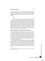
1.13 Block diagram of an analog-to-digital converter. The input analog
voltage is compared with the output of a digital-to-analog converter. When the
two voltages match, the number held in the binary buffer is equivalent to the input
voltage with the resolution of the converter. Different strategies can be used to
adjust the contents of the binary buffer to attain a match.
proportional voltage, V
DAC
. This DAC voltage, V
DAC
, is then compared to the
input voltage, and the binary number in the buffer is adjusted until the desired
level of match between V
DAC
and V
in
is obtained. This approach begs the question
“How are DAC’s constructed?” In fact, DAC’s are relatively easy to construct
using a simple ladder network and the principal of current superposition.
The controller adjusts the binary number based on whether or not the
comparator finds the voltage out of the DAC, V
DAC
, to be greater or less than
the input voltage, V
in
. One simple adjustment strategy is to increase the binary
number by one each cycle if V
DAC
< V

in
, or decrease it otherwise. This so-called
tracking ADC is very fast when V
in
changes slowly, but can take many cycles
when V
in
changes abruptly (Figure 1.14). Not only can the conversion time be
quite long, but it is variable since it depends on the dynamics of the input signal.
This strategy would not easily allow for sampling an analog signal at a fixed
rate due to the variability in conversion time.
An alternative strategy termed successive approximation allows the con-
version to be done at a fixed rate and is well-suited to digital technology. The
successive approximation strategy always takes the same number of cycles irre-
spective of the input voltage. In the first cycle, the controller sets the most
significant bit (MSB) of the buffer to 1; all others are cleared. This binary
number is half the maximum possible value (which occurs when all the bits are
TLFeBOOK
Introduction 23
F
IGURE
1.14 Voltage waveform of an ADC that uses a tracking strategy. The
ADC voltage (solid line) follows the input voltage (dashed line) fairly closely when
the input voltage varies slowly, but takes many cycles to “catch up” to an abrupt
change in input voltage.
1), so the DAC should output a voltage that is half its maximum voltage—that
is, a voltage in the middle of its range. If the comparator tells the controller that
V
in
> V

DAC
, then the input voltage, V
in
, must be greater than half the maximum
range, and the MSB is left set. If V
in
< V
DAC
, then that the input voltage is in the
lower half of the range and the MSB is cleared (Figure 1.15). In the next cycle,
the next most significant bit is set, and the same comparison is made and the
same bit adjustment takes place based on the results of the comparison (Figure
1.15).
After N cycles, where N is the number of bits in the digital output, the
voltage from the DAC, V
DAC
, converges to the best possible fit to the input
voltage, V
in
. Since V
in
Ϸ V
DAC
, the number in the buffer, which is proportional
to V
DAC
, is the best representation of the analog input voltage within the resolu-
tion of the converter. To signal the end of the conversion process, the ADC puts
TLFeBOOK
24 Chapter 1

F
IGURE
1.15 V
in
and V
DAC
in a 6-bit ADC using the successive approximation
strategy. In the first cycle, the MSB is set (solid line) since V
in
> V
DAC
. In the next
two cycles, the bit being tested is cleared because V
in
< V
DAC
when this bit was
set. For the fourth and fifth cycles the bit being tested remained set and for the
last cycle it was cleared. At the end of the sixth cycle a conversion complete flag
is set to signify the end of the conversion process.
out a digital signal or flag indicating that the conversion is complete (Figure
1.15).
TIME SAMPLING: BASICS
Time sampling transforms a continuous analog signal into a discrete time signal,
a sequence of numbers denoted as x(n) = [x
1
, x
2
, x
3

, x
N
],* Figure 1.16 (lower
trace). Such a representation can be thought of as an array in computer memory.
(It can also be viewed as a vector as shown in the next chapter.) Note that the
array position indicates a relative position in time, but to relate this number
sequence back to an absolute time both the sampling interval and sampling onset
time must be known. However, if only the time relative to conversion onset is
important, as is frequently the case, then only the sampling interval needs to be
*In many textbooks brackets, [ ], are used to denote digitized variables; i.e., x[n]. Throughout this
text we reserve brackets to indicate a series of numbers, or vector, following the MATLAB format.
TLFeBOOK
Introduction 25
F
IGURE
1.16 A continuous signal (upper trace) is sampled at discrete points in
time and stored in memory as an array of proportional numbers (lower trace).
known. Converting back to relative time is then achieved by multiplying the
sequence number, n, by the sampling interval, T
s
: x(t) = x(nT
s
).
Sampling theory is discussed in the next chapter and states that a sinusoid
can be uniquely reconstructed providing it has been sampled by at least two
equally spaced points over a cycle. Since Fourier series analysis implies that
any signal can be represented is a series of sin waves (see Chapter 3), then by
extension, a signal can be uniquely reconstructed providing the sampling fre-
quency is twice that of the highest frequency in the signal. Note that this highest
frequency component may come from a noise source and could be well above

the frequencies of interest. The inverse of this rule is that any signal that con-
tains frequency components greater than twice the sampling frequency cannot
be reconstructed, and, hence, its digital representation is in error. Since this error
is introduced by undersampling, it is inherent in the digital representation and
no amount of digital signal processing can correct this error. The specific nature
of this under-sampling error is termed aliasing and is described in a discussion
of the consequences of sampling in Chapter 2.
From a practical standpoint, aliasing must be avoided either by the use of
very high sampling rates—rates that are well above the bandwidth of the analog
system—or by filtering the analog signal before analog-to-digital conversion.
Since extensive sampling rates have an associated cost, both in terms of the
TLFeBOOK
26 Chapter 1
ADC required and memory costs, the latter approach is generally preferable.
Also note that the sampling frequency must be twice the highest frequency
present in the input signal, not to be confused with the bandwidth of the analog
signal. All frequencies in the sampled waveform greater than one half the sam-
pling frequency (one-half the sampling frequency is sometimes referred to as
the Nyquist frequency) must be essentially zero, not merely attenuated. Recall
that the bandwidth is defined as the frequency for which the amplitude is re-
duced by only 3 db from the nominal value of the signal, while the sampling
criterion requires that the value be reduced to zero. Practically, it is sufficient
to reduce the signal to be less than quantization noise level or other acceptable
noise level. The relationship between the sampling frequency, the order of the
anti-aliasing filter, and the system bandwidth is explored in a problem at the
end of this chapter.
Example 1.1. An ECG signal of 1 volt peak-to-peak has a bandwidth of
0.01 to 100 Hz. (Note this frequency range has been established by an official
standard and is meant to be conservative.) Assume that broadband noise may
be present in the signal at about 0.1 volts (i.e., −20 db below the nominal signal

level). This signal is filtered using a four-pole lowpass filter. What sampling
frequency is required to insure that the error due to aliasing is less than −60 db
(0.001 volts)?
Solution. The noise at the sampling frequency must be reduced another
40 db (20 * log (0.1/0.001)) by the four-pole filter. A four-pole filter with a
cutoff of 100 Hz (required to meet the fidelity requirements of the ECG signal)
would attenuate the waveform at a rate of 80 db per decade. For a four-pole
filter the asymptotic attenuation is given as:
Attenuation = 80 log( f
2
/f
c
)db
To achieve the required additional 40 db of attenuation required by the
problem from a four-pole filter:
80 log( f
2
/f
c
) = 40 log( f
2
/f
c
) = 40/80 = 0.5
f
2
/f
c
= 10.5 =;f
2

= 3.16 × 100 = 316 Hz
Thus to meet the sampling criterion, the sampling frequency must be at
least 632 Hz, twice the frequency at which the noise is adequately attenuated.
The solution is approximate and ignores the fact that the initial attenuation of
the filter will be gradual. Figure 1.17 shows the frequency response characteris-
tics of an actual 4-pole analog filter with a cutoff frequency of 100 Hz. This
figure shows that the attenuation is 40 db at approximately 320 Hz. Note the
high sampling frequency that is required for what is basically a relatively low
frequency signal (the ECG). In practice, a filter with a sharper cutoff, perhaps
TLFeBOOK
Introduction 27
F
IGURE
1.17 Detailed frequency plot (on a log-log scale) of a 4-pole and 8-pole
filter, both having a cutoff frequency of 100 Hz.
an 8-pole filter, would be a better choice in this situation. Figure 1.17 shows
that the frequency response of an 8-pole filter with the same 100 Hz frequency
provides the necessary attenuation at less than 200 Hz. Using this filter, the
sampling frequency could be lowered to under 400 Hz.
FURTHER STUDY: BUFFERING
AND REAL-TIME DATA PROCESSING
Real-time data processing simply means that the data is processed and results
obtained in sufficient time to influence some ongoing process. This influence
may come directly from the computer or through human intervention. The pro-
cessing time constraints naturally depend on the dynamics of the process of
interest. Several minutes might be acceptable for an automated drug delivery
system, while information on the electrical activity the heart needs to be imme-
diately available.
TLFeBOOK
28 Chapter 1

The term buffer, when applied digital technology, usually describes a set
of memory locations used to temporarily store incoming data until enough data
is acquired for efficient processing. When data is being acquired continuously,
a technique called double buffering can be used. Incoming data is alternatively
sent to one of two memory arrays, and the one that is not being filled is pro-
cessed (which may involve simply transfer to disk storage). Most ADC software
packages provide a means for determining which element in an array has most
recently been filled to facilitate buffering, and frequently the ability to determine
which of two arrays (or which half of a single array) is being filled to facilitate
double buffering.
DATA BANKS
With the advent of the World Wide Web it is not always necessary to go through
the analog-to-digital conversion process to obtain digitized data of physiological
signals. A number of data banks exist that provide physiological signals such as
ECG, EEG, gait, and other common biosignals in digital form. Given the volatil-
ity and growth of the Web and the ease with which searches can be made, no
attempt will be made to provide a comprehensive list of appropriate Websites.
However, a good source of several common biosignals, particularly the ECG, is
the Physio Net Data Bank maintained by MIT—sionet.o rg. Some
data banks are specific to a given set of biosignals or a given signal proces sing
approach. An example of the latter is the ICALAB Data Bank in Japan—http://
www.bsp.brain .rike n.go. jp/ICALAB/—which includes data that can be used to
evaluate independent component analy sis (s ee Chapter 9) algorithms.
Numerous other data banks containing biosignals and/or images can be
found through a quick search of the Web, and many more are likely to come
online in the coming years. This is also true for some of the signal processing
algorithms as will be described in more detail later. For example, the ICALAB
Website mentioned above also has algorithms for independent component analy-
sis in MATLAB m-file format. A quick Web search can provide both signal
processing algorithms and data that can be used to evaluate a signal processing

system under development. The Web is becoming an evermore useful tool in
signal and image processing, and a brief search of the Web can save consider-
able time in the development process, particularly if the signal processing sys-
tem involves advanced approaches.
PROBLEMS
1. A single sinusoidal signal is contained in noise. The RMS value of the noise
is 0.5 volts and the SNR is 10 db. What is the peak-to-peak amplitude of the
sinusoid?
TLFeBOOK
Introduction 29
2. A resistor produces 10 µV noise when the room temperature is 310°K and
the bandwidth is 1 kHz. What current noise would be produced by this resistor?
3. The noise voltage out of a 1 MΩ resistor was measured using a digital volt
meter as 1.5 µV at a room temperature of 310 °K. What is the effective band-
width of the voltmeter?
4. The photodetector shown in Figure 1.4 has a sensitivity of 0.3µA/µW (at a
wavelength of 700 nm). In this circuit, there are three sources of noise. The
photodetector has a dark current of 0.3 nA, the resistor is 10 MΩ, and the
amplifier has an input current noise of 0.01 pA/√
Hz. Assume a bandwidth of
10 kHz. (a) Find the total noise current input to the amplifier. (b) Find the
minimum light flux signal that can be detected with an SNR = 5.
5. A lowpass filter is desired with the cutoff frequency of 10 Hz. This filter
should attenuate a 100 Hz signal by a factor of 85. What should be the order of
this filter?
6. You are given a box that is said to contain a highpass filter. You input a
series of sine waves into the box and record the following output:
Frequency (Hz): 2 10 20 60 100 125 150 200 300 400
V
out

volts rms: .15×10
−7
0.1×10
−3
0.002 0.2 1.5 3.28 4.47 4.97 4.99 5.0
What is the cutoff frequency and order of this filter?
7. An 8-bit ADC converter that has an input range of ± 5 volts is used to
convert a signal that varies between ± 2 volts. What is the SNR of the input if
the input noise equals the quantization noise of the converter?
8. As elaborated in Chapter 2, time sampling requires that the maximum fre-
quency present in the input be less than f
s
/2 for proper representation in digital
format. Assume that the signal must be attenuated by a factor of 1000 to be
considered “not present.” If the sampling frequency is 10 kHz and a 4th-order
lowpass anti-aliasing filter is used prior to analog-to-digital conversion, what
should be the bandwidth of the sampled signal? That is, what must the cutoff
frequency be of the anti-aliasing lowpass filter?
TLFeBOOK
TLFeBOOK
2
Basic Concepts
NOISE
In Chapter 1 we observed that noise is an inherent component of most measure-
ments. In addition to physiological and environmental noise, electronic noise
arises from the transducer and associated electronics and is intermixed with the
signal being measured. Noise is usually represented as a random variable, x(n).
Since the variable is random, describing it as a function of time is not very
useful. It is more common to discuss other properties of noise such as its proba-
bility distribution, range of variability, or frequency characteristics. While noise

can take on a variety of different probability distributions, the Central Limit
Theorem implies that most noise will have a Gaussian or normal distribution*.
The Central Limit Theorem states that when noise is generated by a large num-
ber of independent sources it will have a Gaussian probability distribution re-
gardless of the probability distribution characteristics of the individual sources.
Figure 2.1A shows the distribution of 20,000 uniformly distributed random
numbers between −1 and +1. The distribution is approximately flat between the
limits of ±1 as expected. When the data set consists of 20,000 numbers, each
of which is the average of two uniformly distributed random numbers, the distri-
bution is much closer to Gaussian (Figure 2.1B, upper right). The distribution
*Both terms are used and reader should be familiar with both. We favor the term “Gaussian” to
avoid the value judgement implied by the word “normal.”
31
TLFeBOOK
32 Chapter 2
F
IGURE
2.1 (A) The distribution of 20,000 uniformly distributed random numbers.
(B) The distribution of 20,000 numbers, each of which is the average of two uni-
formly distributed random numbers. (C) and (D) The distribution obtained when
3 and 8 random numbers, still uniformly distributed, are averaged together. Al-
though the underlying distribution is uniform, the averages of these uniformly dis-
tributed numbers tend toward a Gaussian distribution (dotted line). This is an
example of the Central Limit Theorem at work.
constructed from 20,000 numbers that are averages of only 8 random numbers
appears close to Gaussian, Figure 2.1D, even though the numbers being aver-
aged have a uniform distribution.
The probability of a Gaussianly distributed variable, x, is specified in the
well-known normal or Gaussian distribution equation:
p(x) =

1
σ
√
2π
e
−x
2
/2σ
2
(1)
TLFeBOOK
Basic Concepts 33
Two important properties of a random variable are its mean, or average
value, and its variance, the term σ
2
in Eq. (1). The arithmetic quantities of
mean and variance are frequently used in signal processing algorithms, and their
computation is well-suited to discrete data.
The mean value of a discrete array of N samples is evaluated as:
x
¯
=
1
N
∑
N
k=1
x
k
(2)

Note that the summation in Eq. (2) is made between 1 and N as opposed
to 0 and N − 1. This protocol will commonly be used throughout the text to be
compatible with MATLAB notation where the first element in an array has an
index of 1, not 0.
Frequently, the mean will be subtracted from the data sample to provide
data with zero mean value. This operation is partic ularl y easy in MATLAB as
described in the next section. The sample variance, σ
2
, is calculated as shown in
Eq. (3) below, and the standard de viati on, σ, is just the square root of the varian ce.
σ
2
=
1
N − 1
∑
N
k=1
(x
k
− x
¯
)
2
(3)
Normalizing the standard deviation or variance by 1/N − 1 as in Eq. (3)
produces the best estimate of the variance, if x is a sample from a Gaussian
distribution. Alternatively, normalizing the variance by 1/N produces the second
moment of the data around x. Note that this is the equivalent of the RMS value
of the data if the data have zero as the mean.

When multiple measurements are made, multiple random variables can be
generated. If these variables are combined or added together, the means add so
that the resultant random variable is simply the mean, or average, of the individ-
ual means. The same is true for the variance—the variances add and the average
variance is the mean of the individual variances:
σ
2
=
1
N
∑
N
k=1
σ
2
k
(4)
However, the standard deviation is the square root of the variance and the
standard deviations add as the
√
N times the average standard deviation [Eq.
(5)]. Accordingly, the mean standard deviation is the average of the individual
standard deviations divided by
√
N [Eq. (6)].
From Eq. (4):
∑
N
k=1
σ

2
k
, hence:
∑
N
k=1
σ
k
=
√
N σ
2
=
√
N σ (5)
TLFeBOOK
34 Chapter 2
Mean Standard Deviation =
1
N
∑
N
k=1
σ
k
=
1
N
√
N σ=

σ
√
N
(6)
In other words, averaging noise from different sensors, or multiple obser-
vations from the same source, will reduce the standard deviation of the noise
by the square root of the number of averages.
In addition to a mean and standard deviation, noise also has a spectral
charact er ist ic—that is, its energy dis tri bu tion may vary with frequ enc y. As shown
below, the frequency characteristics of the noise are related to how well one
instantaneous value of noise correlates with the adjacent instantaneous values:
for digitized data how much one data point is correlated with its neighbors. If
the noise has so much randomness that each point is independent of its neigh-
bors, then it has a flat spectral characteristic and vice versa. Such noise is called
white noise since it, like white light, contains equal energy at all frequencies
(see Figure 1.5). The section on Noise Sources in Chapter 1 mentioned that
most electronic sources produce noise that is essentially white up to many mega-
hertz. When white noise is filtered, it becomes bandlimited and is referred to as
colored noise since, like colored light, it only contains energy at certain frequen-
cies. Colored noise shows some correlation between adjacent points, and this
correlation becomes stronger as the bandwidth decreases and the noise becomes
more monochromatic. The relationshi p between bandwid th and correlatio n of adja-
cent points is explored in the section on autocorrelation.
ENSEMBLE AVERAGING
Eq. (6) indicates that averaging can be a simple, yet powerful signal processing
technique for reducing noise when multiple observations of the signal are possi-
ble. Such multiple observations could come from multiple sensors, but in many
biomedi ca l applica ti ons, the mul tip le obser vat ions come from repeated respons es
to the same stimulus. In ensembl e averag ing , a group, or ensembl e, of time re-
sponses are averaged together on a point-by-point basis; that is, an average

signal is constructed by taking the average, for each point in time, over all
signals in the ensemble (Figure 2.2). A classic biomedical engineering example
of the application of ensemble averaging is the visual evoked response (VER)
in which a visual stimulus produces a small neural signal embedded in the EEG.
Usually this signal cannot be detected in the EEG signal, but by averaging
hundreds of observations of the EEG, time-locked to the visual stimulus, the
visually evoked signal emerges.
There are two essential requirements for the application of ensemble aver-
aging for noise reduction: the ability to obtain multiple observations, and a
reference signal closely time-linked to the response. The reference signal shows
how the multiple observations are to be aligned for averaging. Usually a time
TLFeBOOK
Basic Concepts 35
F
IGURE
2.2 Upper trace s: An ensemble of individual (vergence) eye movement
responses to a step ch ange in st imu lus. Lower trace: T he ensemble average, d is-
placed downward for clarity. The ensemble average is constructed by averaging the
individual responses at each point in time. Hence, the value of the aver age re-
sponse at time T1 (vertical line) is the average of the individual responses at that
time.
signal linked to the stimulus is used. An example of ensemble averaging is
shown in Figure 2.2, and the code used to produce this figure is presented in
the following MATLAB implementation section.
MATLAB IMPLEMENTATION
In MATLAB the mean, variance, and standard deviations are implemented as
shown in the three code lines below.
xm = mean(x); % Evaluate mean of x
xvar = var(x) % Evaluate the variance of x normalizing by
% N-1

TLFeBOOK
36 Chapter 2
xnorm = var(x,1); % Evaluate the variance of x
xstd = std(x); % Evaluate the standard deviation of x,
If
x
is an array (also termed a vector for reasons given later) the output
of these function calls is a scalar representing the mean, variance, or standard
deviation. If
x
is a matrix then the output is a row vector resulting from applying
the appropriate calculation (mean, variance, or standard deviation) to each col-
umn of the matrix.
Example 2.1 below shows the implementation of ensemble averaging that
produced the data in Figure 2.2. The program first loads the eye movement data
(
load verg1
), then plots the ensemble. The ensemble average is determined
using the MATLAB
mean
routine. Note that the data matrix,
data_out,
must
be in the correct orientation (the responses must be in rows) for routine
mean
.
If that were not the case (as in Problem 1 at the end of this chapter), the matrix
transposition operation should be performed*. The ensemble average,
avg
,is

then plotted displaced by 3 degrees to provide a clear view. Otherwise it would
overlay the data.
Example 2.1 Compute and display the Ensemble average of an ensemble
of vergence eye movement responses to a step change in stimulus. These re-
sponses are stored in MATLAB file
verg1.mat
.
% Example 2.1 and Figure 2.2 Load eye movement data, plot
% the data then generate and plot the ensemble average.
%
close all; clear all;
load verg1; % Get eye movement data;
Ts = .005; % Sample interval = 5 msec
[nu,N] = size(data_out); % Get data length (N)
t = (1:N)*Ts; % Generate time vector
%
% Plot ensemble data superimposed
plot(t,data_out,‘k’);
hold on;
%
% Construct and plot the ensemble average
avg = mean(data_out); % Calculate ensemble average
plot(t,avg-3,‘k’); % and plot, separated from
% the other data
xlabel(‘Time (sec)’); % Label axes
ylabel(‘Eye Position’);
*In MATLAB, matrix or vector transposition is indicated by an apostrophe following the variable.
For example if x is a row vector, x′ is a column vector and visa versa. If X is a matrix, X′ is that
matrix with rows and columns switched.
TLFeBOOK

Basic Concepts 37
plot([.43 .43],[0 5],’-k’); % Plot horizontal line
text(1,1.2,‘Averaged Data’); % Label data average
DATA FUNCTIONS AND TRANSFORMS
To mathematicians, the term function can take on a wide range of meanings. In
signal processing, most functions fall into two categories: waveforms, images,
or other data; and entities that operate on waveforms, images, or other data
(Hubbard, 1998). The latter group can be further divided into functions that
modify the data, and functions used to analyze or probe the data. For example,
the basic filters described in Chapter 4 use functions (the filter coefficients) that
modify the spectral content of a waveform while the Fourier Transform detailed
in Chapter 3 uses functions (harmonically related sinusoids) to analyze the spec-
tral content of a waveform. Functions that modify data are also termed opera-
tions or transformations.
Since most signal processing operations are implemented using digital
electronics, functions are represented in discrete form as a sequence of numbers:
x(n) = [x(1),x(2),x(3), ,x(N)] (5)
Discret e data fu nct io ns (wavefor ms or images) are usuall y obtained throug h
analog-to-digital conversion or other data input, while analysis or modifying
functions are generated within the computer or are part of the computer pro-
gram. (The consequences of converting a continuous time function into a dis-
crete representation are described in the section below on sampling theory.)
In some applications, it is advantageous to think of a function (of whatever
type) not j ust as a se qu enc e, or arr ay, of numbe rs, but as a v ect or . In this c on cep tu -
alizati on , x(n) is a single vector defined by a single point, the endpoint of the
vector, in N-dimensional space, Figure 2.3. This somewhat curious and highly
mathematical concept has the advantage of unifying some signal processing
operations and fits well with matrix methods. It is difficult for most people to
imagine higher-dimensional spaces and even harder to present them graphically,
so operations and functions in higher-dimensional space are usually described

in 2 or 3 dimensions, and the extension to higher dimensional space is left to
the imagination of the reader. (This task can sometimes be difficult for non-
mathematicians: try and imagine a data sequence of even a 32-point array repre-
sented as a single vector in 32-dimensional space!)
A transform can be thought of as a re-mapping of the original data into a
function that provides more information than the original.* The Fourier Trans-
form described in Chapter 3 is a classic example as it converts the original time
*Some definitions would be more restrictive and require that a transform be bilateral; that is, it
must be possible to recover the original signal from the transformed data. We will use the looser
definition and reserve the term bilateral transform to describe reversible transformations.
TLFeBOOK
38 Chapter 2
F
IGURE
2.3 The data sequence x(n) = [1.5,2.5,2] represented as a vector in
three-dimensional space.
data into frequency information which often provides greater insight into the
nature and/or origin of the signal. Many of the transforms described in this text
are achieved by comparing the signal of interest with some sort of probing
function. This comparison takes the form of a correlation (produced by multipli-
cation) that is averaged (or integrated) over the duration of the waveform, or
some portion of the waveform:
X(m) =
∫
∞
−∞
x(t) f
m
(t)dt (7)
where x(t) is the waveform being analyzed, f

m
(t) is the probing function and m
is some variable of the probing function, often specifying a particular member
in a family of similar functions. For example, in the Fourier Transform f
m
(t)is
a family of harmonically related sinusoids and m specifies the frequency of an
TLFeBOOK
Basic Concepts 39
individual sinusoid in that family (e.g., sin(mft) ). A family of probing functions
is also termed a basis. For discrete functions, a probing function consists of a
sequence of values, or vector, and the integral becomes summation over a finite
range:
X(m) =
∑
N
n=1
x(n)f
m
(n)(8)
where x(n) is the discrete waveform and f
m
(n) is a discrete version of the family
of probing functions. This equation assumes the probe and waveform functions
are the same length. Other possibilities are explored below.
When either x(t)orf
m
(t) are of infinite length, they must be truncated in
some fashion to fit within the confines of limited memory storage. In addition,
if the length of the probing function, f

m
(n), is shorter than the waveform, x(n),
then x(n) must be shortened in some way. The length of either function can be
shortened by simple truncation or by multiplying the function by yet another
function that has zero value beyond the desired length. A function used to
shorten another function is termed a window function, and its action is shown
in Figure 2.4. Note that simple truncation can be viewed as multiplying the
function by a rectangular window, a function whose value is one for the portion
of the function that is retained, and zero elsewhere. The consequences of this
artificial shortening will depend on the specific window function used. Conse-
quences of data windowing are discussed in Chapter 3 under the heading Win-
dow Functions. If a window function is used, Eq. (8) becomes:
X(m) =
∑
N
n=1
x(n) f
m
(n) W(n) (9)
where W(n) is the window function. In the Fourier Transform, the length of
W(n) is usually set to be the same as the available length of the waveform, x(n),
but in other applications it can be shorter than the waveform. If W(n) is a rectan-
gular function, then W(n) =1 over the length of the summation (1 ≤ n ≤ N), and
it is usually omitted from the equation. The rectangular window is implemented
implicitly by the summation limits.
If the probing function is of finite length (in mathematical terms such a
function is said to have finite support) and this length is shorter than the wave-
form, then it might be appropriate to translate or slide it over the signal and
perform the comparison (correlation, or multiplication) at various relative posi-
tions between the waveform and probing function. In the example shown in

Figure 2.5, a single probing function is shown (representing a single family
member), and a single output function is produced. In general, the output would
be a family of functions, or a two-variable function, where one variable corre-
sponds to the relative position between the two functions and the other to the
TLFeBOOK
40 Chapter 2
F
IGURE
2.4 A waveform (upper plot) is multiplied by a window function (middle
plot) to create a truncated version (lower plot) of the original waveform. The win-
dow function is shown in the middle plot. This particular window function is called
the Kaiser Window, one of many popular window functions.
specific family member. This sliding comparison is similar to convolution de-
scribed in the next section, and is given in discrete form by the equation:
X(m,k) =
∑
N
n=1
x(n) f
m
(n − k) (10)
where the variable k indicates the relative position between the two functions
and m is the family member as in the above equations. This approach will be
used in the filters described in Chapter 4 and in the Continuous Wavelet Trans-
form described in Chapter 7. A variation of this approach can be used for
long—or even infinite—probing functions, provided the probing function itself
is shortened by windowing to a length that is less than the waveform. Then the
shortened probing function can be translated across the waveform in the same
manner as a probing function that is naturally short. The equation for this condi-
tion becomes:

TLFeBOOK
Basic Concepts 41
F
IGURE
2.5 The probing function slides over the waveform of interest (upper
panel) and at each position generates the summed, or averaged, product of the
two functions (lower panel), as in Eq. (10). In this example, the probing function
is one member of the “Mexican Hat” family (see Chapter 7) and the waveform is
a sinusoid that increases its frequency linearly over time (known as a chirp.) The
summed product (lower panel), also known as the scalar product, shows the rela-
tive correlation between the waveform and the probing function as it slides across
the waveform. Note that this relative correlation varies sinusoidally as the phase
between the two functions varies, but reaches a maximum around 2.5 sec, the
time when the waveform is most like the probing function.
TLFeBOOK
42 Chapter 2
X(m,k) =
∑
N
n=1
x(n)[W(n − k) f
m
(n)] (11)
where f
m
(n) is a longer function that is shortened by the sliding window function,
(W(n − k), and the variables m and k have the same meaning as in Eq. (10).
This is the approach taken in the Short-Term Fourier Transform described in
Chapter 6.
All of the discrete equations above, Eqs. (7) to (11), have one thing in

common: they all feature the multiplication of two (or sometimes three) func-
tions and the summation of the product over some finite interval. Returning to
the vector conceptualization for data sequences mentioned above (see Figure
2.3), this multiplication and summation is the same as scalar product of the two
vectors.*
The scalar product is defined as:
Scalar product ofa&b≡〈a,b〉=
ͫ
a
1
a
2
Ӈ
a
n
ͬͫ
b
1
b
2
Ӈ
b
n
ͬ
= a
1
b
1
+ a
2

b
2
+

+ a
n
b
n
(12)
Note that the scalar product results in a single number (i.e., a scalar), not
a vector. The scalar product can also be defined in terms of the magnitude of
the two vectors and the angle between them:
Scalar product of a and b ≡〈a,b〉=*a**b* cos θ (13)
where θ is the angle between the two vectors. If the two vectors are perpendicu-
lar to one another, i.e., they are orthogonal, then θ=90°, and their salar product
will be zero. Eq. (13) demonstrates that the scalar product between waveform
and probe function is mathematically the same as a projection of the waveform
vector onto the probing function vector (after normalizing by probe vector
length). When the probing function consists of a family of functions, then the
scalar product operations in Eqs. (7)–(11) can be thought of as projecting the
waveform vector onto vectors representing the various family members. In this
vector-based conceptualization, the probing function family, or basis, can be
thought of as the axes of a coordinate system. This is the motivation behind the
development of probing functions that have family members that are orthogonal,
*The scalar product is also termed the inner product, the standard inner product,orthedot
product.
TLFeBOOK
Basic Concepts 43
or orthonormal:† the scalar product computations (or projections) can be done
on each axes (i.e., on each family member) independently of the others.

CONVOLUTION, CORRELATION, AND COVARIANCE
Convolution, correlation, and covariance are similar-sounding terms and are
similar in the way th ey are calcula ted . This similar ity is somewhat misleading—at
least in the ca se of convol ut ion—since the areas of appl ic ation and underlying
concepts are not the same.
Convolution and the Impulse Response
Convolution is an important concept in linear systems theory, solving the need
for a time domain operation equivalent to the Transfer Function. Recall that the
Transfer Function is a frequency domain concept that is used to calculate the
output of a linear system to any input. Convolution can be used to define a
general input–output relationship in the time domain analogous to the Transfer
Function in the frequency domain. Figure 2.6 demonstrates this application of
convolution. The input, x(t), the output, y(t), and the function linking the two
through convolution, h(t), are all functions of time; hence, convolution is a time
domain operation. (Ironically, convolution algorithms are often implemented in
the frequency domain to improve the speed of the calculation.)
The basic concept behind convolution is superposition. The first step is to
determine a time function, h(t), that tells how the system responds to an infi-
nitely short segment of the input waveform. If superposition holds, then the
output can be determined by summing (integrating) all the response contribu-
tions calculated from the short segments. The way in which a linear system
responds to an infinitely short segment of data can be determined simply by
noting the system’s response to an infinitely short input, an infinitely short
pulse. An infinitely short pulse (or one that is at least short compared to the
dynamics of the system) is termed an impulse or delta function (commonly
denoted δ(t)), and the response it produces is termed the impulse response, h(t).
F
IGURE
2.6 Convolution as a linear process.
†Orthonormal vectors are orthogonal, but also have unit length.

TLFeBOOK
44 Chapter 2
Given that the impulse response describes the response of the system to an
infinitely short segment of data, and any input can be viewed as an infinite
string of such infinitesimal segments, the impulse response can be used to deter-
mine the output of the system to any input. The response produced by an infi-
nitely small data segment is simply this impulse response scaled by the magni-
tude of that data segment. The contribution of each infinitely small segment can
be summed, or integrated, to find the response created by all the segments.
The convolution process is shown schematically in Figure 2.7. The left
graph shows the input, x(n) (dashed curve), to a linear system having an impulse
response of h(n) (solid line). The right graph of Figure 2.7 shows three partial
responses (solid curves) produced by three different infinitely small data segments
at N1, N2, and N3. Each partial response is an impulse response scaled by the
associated input segment and shifted to the position of that segment. The output
of the linear process (right graph, dashed line) is the summation of the individual
F
IGURE
2.7 (A) The input, x(n), to a linear system (dashed line) and the impulse
response of that system, h(n) (solid line). Three points on the input data se-
quence are shown: N1, N2, and N3. (B) The partial contributions from the three
input data points to the output are impulse responses scaled by the value of the
associated input data point (solid line). The overall response of the system, y(n)
(dashed line, scaled to fit on the graph), is obtained by summing the contributions
from all the input points.
TLFeBOOK
Basic Concepts 45
impulse responses produced by each of the input data segments. (The output is
scaled down to produce a readable plot).
Stated mathematically, the output y(t), to any input, x(t) is given by:

y(t) =
∫
+∞
−∞
h(τ) x(t −τ)dτ=
∫
+∞
−∞
h(t −τ) x(τ)dτ (14)
To determine the impulse of each infinitely small data segment, the im-
pulse response is shifted a time τ with respect to the input, then scaled (i.e.,
multiplied) by the magnitude of the input at that point in time. It does not matter
which function, the input or the impulse response, is shifted.* Shifting and mul-
tiplication is sometimes referred to as the lag product. For most systems, h(τ)
is finite, so the limit of integration is finite. Moreover, a real system can only
respond to past inputs, so h(τ)mustbe0forτ<0 (negative τ impli es future times
in Eq. (14), although for computer-based operations, where future data may be
available in memory, τ can be negative.
For discrete signals, the integration becomes a summation and the convo-
lution equation becomes:
y(n) =
∑
N
k=1
h(n − k) x(k) or
y(n) =
∑
N
k=1
h(n) x(k − n) ≡ h(n)*x(n) (15)

Again either h(n)orx(n) can be shifted. Also for discrete data, both h(n)
and x(n) must be finite (since they are stored in finite memory), so the summa-
tion is also finite (where N is the length of the shorter function, usually h(n)).
In signal processing, convolution can be used to implement some of the
basic filters described in Chapter 4. Like their analog counterparts, digital filters
are just linear processes that modify the input spectra in some desired way (such
as reducing noise). As with all linear processes, the filter’s impulse response,
h(n), completely describes the filter. The process of sampling used in analog-
to-digital conversion can also be viewed in terms of convolution: the sampled
output x(n) is just the convolution of the analog signal, x(t ), with a very short
pulse (i.e., an impulse function) that is periodic with the sampling frequency.
Convolution has signal processing implications that extend beyond the determi-
nation of input-output relationships. We will show later that convolution in the
time domain is equivalent to multiplication in the frequency domain, and vice
versa. The former has particular significance to sampling theory as described
latter in this chapter.
*Of course, shifting both would be redundant.
TLFeBOOK
46 Chapter 2
Covariance and Correlation
The word correlation connotes similarity: how one thing is like another. Mathe-
matically, correlations are obtained by multiplying and normalizing. Both covar-
iance and correlation use multiplication to compare the linear relationship be-
tween two variables, but in correlation the coefficients are normalized to fall
between zero and one. This makes the correlation coefficients insensitive to
variations in the gain of the data acquisition process or the scaling of the vari-
ables. However, in many signal processing applications, the variable scales are
similar, and covariance is appropriate. The operations of correlation and covari-
ance can be applied to two or more waveforms, to multiple observations of the
same source, or to multiple segments of the same waveform. These comparisons

between data sequences can also result in a correlation or covariance matrix as
described below.
Correlation/covariance operations can not only be used to compare differ-
ent waveforms at specific points in time, they can also make comparisons over
a range of times by shifting one signal with respect the other. The crosscorrela-
tion function is an example of this process. The correlation function is the lagged
product of two waveforms, and the defining equation, given here in both contin-
uous and discrete form, is quite similar to the convolution equation above (Eqs.
(14) and (15):
r
xx
(t) =
∫
T
0
y(t) x(t +τ)dτ (16a)
r
xx
(n) =
∑
M
k=1
y(k + n) x(k) (16b)
Eqs. (16a) and (16b) show that the only difference in the computation of
the crosscorrelation versus convolution is the direction of the shift. In convolu-
tion the waveforms are shifted in opposite directions. This produces a causal
output: the output function is the creation of past values of the input function
(the output is caused by the input). This form of shifting is reflected in the
negative sign in Eq. (15). Crosscorrelation shows the similarity between two
waveforms at all possible relative positions of one waveform with respect to

the other, and it is useful in identifying segments of similarity. The output of
Eq. (16) is sometimes termed the raw correlation since there is no normaliza-
tion involved. Various scalings can be used (such as dividing by N, the number
of in the sum), and these are described in the section on MATLAB implementa-
tion.
A special case of the correlation function occurs when the comparison is
between two waveforms that are one in the same; that is, a function is correlated
with different shifts of itself. This is termed the autocorrelation function and it
TLFeBOOK