Biosignal and Biomedical Image Processing phần 4 pot

Digital Filters 105
wh = .3 * pi; % Set bandpass cutoff
% frequencies
wl = .1*pi;
L = 128; % Number of coeffients
% equals 128
for i = 1:L؉1 % Generate bandpass
% coefficient function
n = i-L/2 ; % and make symmetrical
if n == 0
bn(i) = wh/pi-wl/pi;
else
bn(i) = (sin(wh*n))/(pi*n)-(sin(wl*n))/(pi*n) ;
% Filter impulse response
end
end
bn = bn .* blackman(L؉1)’; % Apply Blackman window
% to filter coeffs.
H_data = abs(fft(data)); % Plot data spectrum for
% comparison
freq = (1:N/2)*fs/N; % Frequency vector for
% plotting
plot(freq,H_data(1:N/2),’k’); % Plot data FFT only to
%fs/2
hold on;
%
H = abs(fft(bn,N)); % Find the filter
% frequency response
H = H*1.2 * (max(H_data)/max(H)); % Scale filter H(z) for
% comparison
plot(freq,H(1:N/2),’ k’); % Plot the filter

% frequency response
xlabel(’Frequency (Hz)’); ylabel(’H(f)’);
y = conv(data,bn); % Filter the data using
% convolution
figure;
t = (1:N)/fs; % Time vector for
% plotting
subplot(2,1,1);
plot(t(1:N/2),data(1:N/2),’k’) % Plot only 1/2 of the
% data set for clarity
xlabel(’Time (sec)’) ;ylabel(’EEG’);
subplot(2,1,2); % Plot the bandpass
% filtered data
plot (t(1:N/2), y(1:N/2),’k’);
ylabel(’Time’); ylabel(’Filtered EEG’);
TLFeBOOK
106 Chapter 4
In this example, the initial loop constructs the filter weights based on Eq.
(12). The filter has high and low cutoff frequencies of 0.1π and 0.3 π radians/
sample, or 0.1f
s
/2 and 0.3f
s
/2 Hz. Assuming a sampling frequency of 100 Hz
this would correspond to cutoff frequencies of 5 to 15 Hz. The FFT is also used
to evaluate the filter’s frequency response. In this case the coefficient function
is zero-padded to 1000 points both to improve the appearance of the frequency
response curve and to match the data length. A frequency vector is constructed
to plot the correct frequency range based on a sampling frequency of 100 Hz.
The bandpass filter is applied to the data using convolution. Two adjustments

must be made when using convolution to implement an FIR filter. If the filter
weighting function is asymmetrical, as with the two-point central difference
algorithm, then the filter order should be reversed to compensate for the way
in which convolution applies the weights. In all applications, the MATLAB
convolution ro utine generates additional points (N = length(data) + leng th(b(n) −
1) so the output must be shortened to N points. Here the initial N points are
taken, but other strategies are mentioned in Chapter 2. In this example, only the
first half of the data set is plotted in Figure 4.11 to improve clarity.
Comparing the unfiltered and filtered data in Figure 4.11, note the sub-
stantial differences in appearance despite the fact that only a small potion of the
signal’s spectrum is attenuated. Particularly apparent is the enhancement of the
oscillatory component due to the suppression of the lower frequencies. This
figure shows that even a moderate amount of filtering can significantly alter the
appearance of the data. Also note the 50 msec initial transient and subsequent
phase shift in the filtered data. This could be corrected by shifting the filtered
data the appropriate number of sample points to the left.
INFINITE IMPULSE RESPONSE (IIR) FILTERS
The primary advantage of IIR filters over FIR filters is that they can usually
meet a specific frequency criterion, such as a cutoff sharpness or slope, with a
much lower filter order (i.e., a lower number of filter coefficients). The transfer
function of IIR filters includes both numerator and denominator terms (Eq. (4))
unlike FIR filters which have only a numerator. The basic equation for the IIR
filter is the same as that for any general linear process shown in Eq. (6) and
repeated here with modified limits:
y(k) =
∑
L
N
n=1
b(n) x(k − n) −

∑
L
D
n=1
a(n) y(k − n) (18)
where b(n) is the numerator coefficients also found in FIR filters, a(n)isthe
denominator coefficients, x(n) is the input, and y(n) the output. While the b(n)
coefficients operate only on values of the input, x (n), the a(n) coefficients oper-
TLFeBOOK
Digital Filters 107
ate on passed values of the output, y(n) and are, therefore, sometimes referred
to as recursive coefficients.
The major disadvantage of IIR filters is that they have nonlinear phase
characteristics. However if the filtering is done on a data sequence that totally
resides in computer memory, as is often the case, than so-called noncausal
techniques can be used to produce zero phase filters. Noncausal techniques use
both future as well as past data samples to eliminate phase shift irregularities.
(Since these techniques use future data samples the entire waveform must be
available in memory.) The two-point central difference algorithm with a positive
skip factor is a noncausal filter. The Signal Processing Toolbox routine
filt-
filt
described in the next section utilizes these noncausal methods to imple-
ment IIR (or FIR) filters with no phase distortion.
The design of IIR filters is not as straightforward as FIR filters; however,
the MATLAB Signal Processing Toolbox provides a number of advanced rou-
tines to assist in this process. Since IIR filters have transfer functions that are
the same as a general linear process having both poles and zeros, many of the
concepts of analog filter design can be used with these filters. One of the most
basic of these is the relationship between the number of poles and the slope, or

rolloff of the filter beyond the cutoff frequency. As mentioned in Chapter 1, the
asymptotic downward slope of a filter increases by 20 db/decade for each filter
pole, or filter order. Determining the number of poles required in an IIR filter
given the desired attenuation characteristic is a straightforward process.
Another similarity between analog and IIR digital filters is that all of the
well-known analog filter types can be duplicated as IIR filters. Specifically the
Butterworth, Chebyshev Type I and II, and elliptic (or Cauer) designs can be
implemented as IIR digital filters and are supported in the MATLAB Signal
Processing Toolbox. As noted in Chapter 1, Butterworth filters provide a fre-
quency response that is maximally flat in the passband and monotonic overall.
To achieve this characteristic, Butterworth filters sacrifice rolloff steepness;
hence, the Butterworth filter will have a less sharp initial attenuation characteris-
tic than other filters. The Chebyshev Type I filters feature faster rolloff than
Butterworth filters, but have ripple in the passband. Chebyshev Type II filters
have ripple only in the stopband and a monotonic passband, but they do not
rolloff as sharply as Type I. The ripple produced by Chebyshev filters is termed
equi-ripple since it is of constant amplitude across all frequencies. Finally, ellip-
tic filters have steeper rolloff than any of the above, but have equi-ripple in both
the passband and stopband. In general, elliptic filters meet a given performance
specification with the lowest required filter order.
Implementation of IIR filters can be achieved using the
filter
function
described above. Design of IIR filters is greatly facilitated by the Signal Process-
ing Toolbox as described below. This Toolbox can also be used to design FIR
filters, but is not essential in implementing these filters. However, when filter
TLFeBOOK
108 Chapter 4
requirements call for complex spectral characteristics, the use of the Signal Pro-
cessing Toolbox is of considerable value, irrespective of the filter type. The

design of FIR filters using this Toolbox will be covered first, followed by IIR
filter design.
FILTER DESIGN AND APPLICATION USING THE MATLAB
SIGNAL PROCESSING TOOLBOX
FIR Filters
The MATLAB Signal Processing Toolbox includes routines that can be used to
apply both FIR and IIR filters. While they are not necessary for either the design
or application of FIR filters, they do ease the design of both filter types, particu-
larly for filters with complex frequency characteristics or demanding attenuation
requirements. Within the MATLAB environment, filter design and application
occur in either two or three stages, each stage executed by separate, but related
routines. In the three-stage protocol, the user supplies information regarding the
filter type and desired attenuation characteristics, but not the filter order. The
first-stage routines determine the appropriate order as well as other parameters
required by the second-stage routines. The second stage routines generate the
filter coefficients, b(n), based the arguments produced by the first-stage routines
including the filter order. A two-stage design process would start with this stage,
in which case the user would supply the necessary input arguments including
the filter order. Alternatively, more recent versions of MATLAB’s Signal Pro-
cessing Toolbox provide an interactive filter design package called FDATool
(for filter design and analysis tool) which performs the same operations de-
scribed below, but utilizing a user-friendly graphical user interface (GUI). An-
other Signal Processing Toolbox package, the SPTool (signal processing tool)
is useful for analyzing filters and generating spectra of both signals and filters.
New MATLAB releases contain detailed information of the use of these two
packages.
The final stage is the same for all filters including IIR filters: a routine
that takes the filter coefficients generated by the previous stage and applies them
to the data. In FIR filters, the final stage could be implemented using convolu-
tion as was done in previous examples, or the MATLAB

filter
routine de-
scribed earlier, or alternatively the MATLAB Signal Processing Toolbox routine
filtfilt
can be used for improved phase properties.
One useful Signal Processing Toolbox routine determines the frequency
response of a filter given the coefficients. Of course, this can be done using the
FFT as shown in Examples 4.2 and 4.3, and this is the approach used by the
MATLAB routine. However the MATLAB routine
freqz
, also includes fre-
quency scaling and plotting, making it quite convenient. The
freqz
routine
TLFeBOOK
Digital Filters 109
plots, or produces, both the magnitude and the phase characteristics of a filter’s
frequency response:
[h,w] = freqz (b,a,n,fs);
where again
b
and
a
are the filter coefficients and
n
is the number of points in
the desired frequency spectra. Setting
n
as a power of 2 is recommended to
speed computation (the default is 512). The input argument,

fs
, is optional and
specifies the sampling frequency. Both output arguments are also optional: if
freqz
is called without the output arguments, the magnitude and phase plots
are produced. If specified, the output vector
h
is the n-point complex frequency
response of the filter. The magnitude would be equal to
abs(h)
while the phase
would be equal to
angle(h)
. The second output argument,
w
, is a vector the
same length as h containing the frequencies of h and is useful in plotting. If
fs
is given,
w
is in Hz and ranges between 0 and f
s
/2; otherwise
w
is in rad/sample
and ranges between 0 and π.
Two-Stage FIR Filter Design
Two-stage filter design requires that the designer known the filter order, i.e.,
the number of coefficients in b(n), but otherwise the design procedure is
straightforward. The MATLAB Signal Processing Toolbox has two filter design

routines based on the rectangular filters described above, i.e., Eqs. (10)–(13).
Although implementation of these equations using standard MATLAB code is
straightforward (as demonstrated in previous examples), the FIR design routines
replace many lines of MATLAB code with a single routine and are seductively
appealing. While both routines are based on the same approach, one allows
greater flexibility in the specification of the desired frequency curve. The basic
rectangular filter is implemented with the routine
fir1
as:
b = fir1(n,wn,’ftype’ window);
where
n
is the filter order,
wn
the cutoff frequency,
ftype
the filter type, and
window
specifies the window function (i.e., Blackman, Hamming, triangular,
etc.). The output,
b
, is a vector containing the filter coefficients. The last two
input arguments are optional. The input argument
ftype
can be either
‘high’
for a highpass filter, or
‘stop’
for a stopband filter. If not specified, a lowpass
or bandpass filter is assumed depending on the length of

wn
. The argument,
window
, is used as it is in the
pwelch
routine: the function name includes argu-
ments specifying window length (see Example 4.3 below) or other arguments.
The window length should equal
n؉1
. For bandpass and bandstop filters,
n
must
be even and is incremented if not, in which case the window length should be
suitably adjusted. Note that MATLAB’s popular default window, the Hamming
TLFeBOOK
110 Chapter 4
window, is used if this argument is not specified. The cutoff frequency is either
a scalar specifying the lowpass or highpass cutoff frequency, or a two-element
vector that specifies the cutoff frequencies of a bandpass or bandstop filter. The
cutoff frequency(s) ranges between 0 and 1 normalized to f
s
/2 (e.g., if,
wn
= 0.5,
then f
c
= 0.5 * f
s
/2). Other options are described in the MATLAB Help file on
this routine.

A related filter design algorithm,
fir2
, is used to design rectangular filters
when a more general, or arbitrary frequency response curve is desired. The
command structure for
fir2
is;
b = fir2(n,f,A,window)
where
n
is the filter order,
f
is a vector of normalized frequencies in ascending
order, and
A
is the desired gain of the filter at the corresponding frequency in
vector
f
. (In other words,
plot(f,A)
would show the desired magnitude fre-
quency curve.) Clearly
f
and
A
must be the same length, but duplicate frequency
points are allowed, corresponding to step changes in the frequency response.
Again, frequency ranges between 0 and 1, normalized to f
s
/2. The argument

window is the same as in
fir1
, and the output,
b
, is the coefficient function.
Again, other optional input arguments are mentioned in the MATLAB Help file
on this routine.
Several other more specialized FIR filters are available that have a two-
stage design protocol. In addition, there is a three-stage FIR filter described in
the next section.
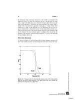
Example 4.4 Design a window-based FIR bandpass filter having the fre-
quency characteristics of the filter developed in Example 4.3 and shown in
Figure 4.12.
% Example 4.4 and Figure 4.12 Design a window-based bandpass
% filter with cutoff frequencies of 5 and 15 Hz.
% Assume a sampling frequency of 100 Hz.
% Filter order = 128
%
clear all; close all;
fs = 100; % Sampling frequency
order = 128; % Filter order
wn = [5*fs/2 15*fs/2]; % Specify cutoff
% frequencies
b = fir1(order,wn); % On line filter design,
% Hamming window
[h,freq] = freqz(b,1,512,100); % Get frequency response
plot(freq,abs(h),’k’); % Plot frequency response
xlabel(’Frequency (Hz)’); ylabel(’H(f)’);
TLFeBOOK
Digital Filters 111

F
IGURE
4.12 The frequency response of an FIR filter based in the rectangular
filter design described in Eq. (10). The cutoff frequencies are 5 and 15 Hz. The
frequency response of this filter is identical to that of the filter developed in Exam-
ple 4.5 and presented in Figure 4.10. However, the development of this filter
required only one line of code.
Three-Stage FIR Filter Design
The first stage in the three-stage design protocol is used to determine the filter
order and cutoff frequencies to best approximate a desired frequency response
curve. Inputs to these routines specify an ideal frequency response, usually as a
piecewise approximation and a maximum deviation from this ideal response.
The design routine generates an output that includes the number of stages re-
quired, cutoff frequencies, and other information required by the second stage.
In the three-stage design process, the first- and second-stage routines work to-
gether so that the output of the first stage can be directly passed to the input of
the second-stage routine. The second-stage routine generates the filter coeffi-
cient function based on the input arguments which include the filter order, the
cutoff frequencies, the filter type (generally optional), and possibly other argu-
ments. In cases where the filter order and cutoff frequencies are known, the
TLFeBOOK
112 Chapter 4
first stage can be bypassed and arguments assigned directly to the second-stage
routines. This design process will be illustrated using the routines that imple-
ment Parks–McClellan optimal FIR filter.
The first design stage, the determination of filter order and cutoff frequen-
cies uses the MATLAB routine
remezord
. (First-stage routines end in the letters
ord

which presumably stands for filter order). The calling structure is
[n, fo, ao, w] = remezord (f,a,dev,Fs);
The input arguments,
f
,
a
and
dev
specify the desired frequency response
curve in a somewhat roundabout manner.
Fs
is the sampling frequency and is
optional (the default is 2 Hz so that f
s
/2 = 1 Hz). Vector
f
specifies frequency
ranges between 0 and f
s
/2 as a pair of frequencies while
a
specifies the desired
gains within each of these ranges. Accordingly,
f
has a length of
2n—2
, where
n
is the length of
a

. The
dev
vector specifies the maximum allowable deviation,
or ripple, within each of these ranges and is the same length as
a
. For example,
assume you desire a bandstop filter that has a passband between 0 and 100 with
a ripple of 0.01, a stopband between 300 and 400 Hz with a gain of 0.1, and an
upper passband between 500 and 1000 Hz (assuming f
s
/2 = 1000) with the same
ripple as the lower passband. The
f
,
a
, and
dev
vectors would be:
f = [100
300 400 500]
;
a = [101]
; and
dev = [.01 .1 .01]
. Note that the ideal
stopband gain is given as zero by vector
a
while the actual gain is specified by
the allowable deviation given in vector
dev

. Vector
dev
requires the deviation
or ripple to be specified in linear units not in db. The application of this design
routine is shown in Example 4.5 below.
The output arguments include the required filter order,
n
, the normalized
frequency ranges,
fo
, the frequency amplitudes for those ranges,
a0
, and a set
of weights,
w
, that tell the second stage how to assess the accuracy of the fit in
each of the frequency ranges. These four outputs become the input to the second
stage filter design routine
remez
. The calling structure to the routine is:
b = remez (n, f, a, w,’ftype’);
where the first four arguments are supplied by
remezord
although the input
argument
w
is optional. The fifth argument, also optional, specifies either a
hilbert
linear-phase filter (most common, and the default) or a
differentia-

tor
which weights the lower frequencies more heavily so they will be the most
accurately constructed. The output is the FIR coefficients,
b
.
If the desired filter order is known, it is possible to bypass remezord and
input the arguments
n
,
f
, and
a
directly. The input argument,
n
,issimplythe
filter order. Input vectors
f
and
a
specify the desired frequency response curve
in a somewhat different manner than described above. The frequency vector still
contains monotonically increasing frequencies normalized to f
s
/2; i.e., ranging
TLFeBOOK
Digital Filters 113
between 0 and 1 where 1 corresponds to f
s
/2. The
a

vector represents desired
filter gain at each end of a frequency pair, and the gain between pairs is an
unspecified transition region. To take the example above: a bandstop filter that
has a passband (gain = 1) between 0 and 100, a stopband between 300 and 400
Hz with a gain of 0.1, and an upper passband between 500 and 700 Hz; assum-
ing f
s
/2 = 1 kHz, the
f
and a vector would be:
f = [0 .1 .3 .4 .5 .7]; a =
[11.1.111]
. Note that the desired frequency curve is unspecified between
0.1 and 0.3 and also between 0.4 and 0.5.
As another example, assume you wanted a filter that would differentiate
a signal up to 0.2f
s
/2 Hz, then lowpass filter the signal above 0.3f
s
/2 Hz. The
f
and
a
vector would be:
f = [0 .1 .3 1]
;
a = [0100]
.
Another filter that uses the same input structure as
remezord

is the least
square linear-phase filter design routine
firls
. The use of this filter in for
calculation the derivative is found in the Problems.
The following example shows the design of a bandstop filter using the
Parks–McClellan filter in a three-stage process. This example is followed by
the design of a differentiator Parks–McClellan filter, but a two-stage design
protocol is used.
Example 4.5 Design a bandstop filter having the following characteris-
tics: a passband gain of 1 (0 db) between 0 and 100, a stopband gain of −40 db
between 300 and 400 Hz, and an upper passband gain of 1 between 500 and
1000 Hz. Maximum ripple for the passband should be ±1.5 db. Assume f
s
= 2
kHz. Use the three-stage design process. In this example, specifying the
dev
argument is a little more complicated because the requested deviations are given
in db while
remezord
expects linear values.
% Example 4.5 and Figure 4.13
% Bandstop filter with a passband gain of 1 between 0 and 100,
% a stopband gain of -40 db between 300 and 400 Hz,
% and an upper passband gain of 1 between 500 and fs/2 Hz (1000
%Hz).
% Maximum ripple for the passband should be ±1.5 db
%
rp_pass = 3; % Specify ripple
% tolerance in passband

rp_stop = 40; % Specify error
% tolerance in passband
fs = 2000; % Sample frequency: 2
% kHz
f = [100 300 400 500]; % Define frequency
% ranges
a= [1 0 1]; % Specify gain in
% those regions
%
TLFeBOOK
114 Chapter 4
F
IGURE
4.13 The magnitude and phase frequency response of a Parks–McClel-
lan bandstop filter produced in Example 4.5. The number of filter coefficients as
determined by
remezord
was 24.
% Now specify the deviation converting from db to linear
dev = [(10
v
(rp_pass/20)-1)/(10
v
(rp_pass/20)؉1) 10
v
(-rp_stop/20) (10
v
(rp_pass/20)-1)/(10
v
(rp_pass/

20)؉1)];
%
% Design filter - determine filter order
[n, fo, ao, w] = remezord(f,a,dev,fs) % Determine filter
% order, Stage 1
b = remez(n, fo, ao, w); % Determine filter
% weights, Stage 2
freq.(b,1,[ ],fs); % Plot filter fre-
% quency response
In Example 4.5 the vector assignment for the a vector is straightforward:
the desired gain is given as 1 in the passband and 0 in the stopband. The actual
stopband attenuation is given by the vector that specifies the maximum desirable
TLFeBOOK
Digital Filters 115
error, the
dev
vector. The specification of this vector, is complicated by the fact
that it must be given in linear units while the ripple and stopband gain are
specified in db. The db to linear conversion is included in the
dev
assignment.
Note the complicated way in which the passband gain must be assigned.
Figure 4.13 shows the plot produced by
freqz
with no output arguments,
a
= 1,
n
= 512 (the default), and
b

was the FIR coefficient function produced in
Example 4.6 above. The phase plot demonstrates the linear phase characteristics
of this FIR filter in the passband. This will be compared with the phase charac-
teristics of IIR filter in the next section.
The frequency response curves for Figure 4.13 were generated using the
MATLAB routine
freqz
, which applies the FFT to the filter coefficients follow-
ing Eq. (7). It is also possible to generate these curves by passing white noise
through the filter and computing the spectral characteristics of the output. A
comparison of this technique with the direct method used above is found in
Problem 1.
Example 4.6 Design a differentiator using the MATLAB FIR filter
re-
mez
. Use a two-stage design process (i.e., select a 28-order filter and bypass the
first stage design routine
remezord
). Compare the derivative produced by this
signal with that produced by the two-point central difference algorithm. Plot the
results in Figure 4.14.
The FIR derivative operator will be designed by requesting a linearly in-
creasing frequency characteristic (slope = 1) up to some f
c
Hz, then a sharp drop
off within the next 0.1f
s
/2 Hz. Note that to make the initial magnitude slope
equal to 1, the magnitude value at
fc

should be: f
c
* f
s
* π.
% Example 4.6 and Figure 4.14
% Design a FIR derivative filter and compare it to the
% Two point central difference algorithm
%
close all; clear all;
load sig1; % Get data
Ts = 1/200; % Assume a Ts of 5 msec.
fs = 1/Ts; % Sampling frequency
order = 28; % FIR Filter order
L = 4; % Use skip factor of 4
fc = .05 % Derivative cutoff
% frequency
t = (1:length(data))*Ts;
%
% Design filter
f = [0fcfc؉.1 .9]; % Construct desired freq.
% characteristic
TLFeBOOK
116 Chapter 4
F
IGURE
4.14 Derivative produced by an FIR filter (left) and the two-point central
difference differentiator (right). Note that the FIR filter does produce a cleaner
derivative without reducing the value of the peak velocity. The FIR filter order
(n = 28) and deriviative cutoff frequency (f

c
= .05 f
s
/2) were chosen empirically to
produce a clean derivative with a maximal velocity peak. As in Figure 4.5 the
velocity (i.e., derivative) was scaled by
1
/
2
to be more compatible with response
amplitude.
a = [0 (fc*fs*pi) 0 0]; % Upward slope until .05 f
s
% then lowpass
b = remez(order,f,a, % Design filter coeffi-
’differentiator’); % cients and
d_dt1 = filter(b,1,data); % apply FIR Differentiator
figure;
subplot(1,2,1);
hold on;
plot(t,data(1:400)؉12,’k’); % Plot FIR filter deriva-
% tive (data offset)
plot(t,d_dt1(1:400)/2,’k’); % Scale velocity by 1/2
ylabel(’Time(sec)’);
ylabel(’x(t) & v(t)/2’);
TLFeBOOK
Digital Filters 117
%
%
% Now apply two-point central difference algorithm

hn = zeros((2*L)؉1,1); % Set up h(n)
hn(1,1) = 1/(2*L* Ts);
hn((2*L)؉1,1) = -1/(2*L*Ts); % Note filter weight
% reversed if
d_dt2 = conv(data,hn); % using convolution
%
subplot(1,2,2);
hold on;
plot(data(1:400)؉12,’k’); % Plot the two-point cen-
% tral difference
plot(d_dt2(1:400)/2,’k’); % algorithm derivative
ylabel(’Time(sec)’);
ylabel(’x(t) & v(t)/2’);
IIR Filters
IIR filter design under MATLAB follows the same procedures as FIR filter
design; only the names of the routines are different. In the MATLAB Signal
Processing Toolbox, the three-stage design process is supported for most of the
IIR filter types; however, as with FIR design, the first stage can be bypassed if
the desired filter order is known.
The third stage, the application of the filter to the data, can be imple-
mented using the standard
filter
routine as was done with FIR filters. A Signal
Processing Toolbox routine can also be used to implement IIR filters given the
filter coefficients:
y = filtfilt(b,a,x)
The arguments for
filtfilt
are identical to those in
filter

. The only
difference is that
filtfilt
improves the phase performance of IIR filters by
running the algorithm in both forward and reverse directions. The result is a
filtered sequence that has zero-phase distortion and a filter order that is doubled.
The downsides of this approach are that initial transients may be larger and the
approach is inappropriate for many FIR filters that depend on phase response
for proper operations. A comparison between the
filter
and
filtfilt
algo-
rithms is made in the example below.
As with our discussion of FIR filters, the two-stage filter processes will
be introduced first, followed by three-stage filters. Again, all filters can be im-
plemented using a two-stage process if the filter order is known. This chapter
concludes with examples of IIR filter application.
TLFeBOOK
118 Chapter 4
Two-Stage IIR Filter Design
The Yule–Walker recursive filter is the only IIR filter that is not supported by
an order-selection routine (i.e., a three-stage design process). The design routine
yulewalk
allows for the specification of a general desired frequency response
curve, and the calling structure is given on the next page.
[b,a] = yulewalk(n,f,m)
where
n
is the filter order, and

m
and
f
specify the desired frequency characteris-
tic in a fairly straightforward way. Specifically,
m
is a vector of the desired filter
gains at the frequencies specified in
f
. The frequencies in
f
are relative to f
s
/2:
the first point in
f
must be zero and the last point 1. Duplicate frequency points
are allowed and correspond to steps in the frequency response. Note that this is
the same strategy for specifying the desired frequency response that was used
by the FIR routines
fir2
and
firls
(see Help file).
Example 4.7 Design an 12th-order Yule–Walker bandpass filter with
cutoff frequencies of 0.25 and 0.5. Plot the frequency response of this filter and
compare with that produced by the FIR filter
fir2
of the same order.
% Example 4.7 and Figure 4.15

% Design a 12th-order Yulewalk filter and compare
% its frequency response with a window filter of the same
% order
%
close all; clear all;
n = 12; % Filter order
f = [0 .25 .25 .6 .6 1]; % Specify desired frequency re-
% sponse
m = [001100];
[b,a] = yulewalk(n,f,m); % Construct Yule–Walker IIR Filter
h = freqz(b,a,256);
b1 = fir2(n,f,m); % Construct FIR rectangular window
% filter
h1 = freqz(b1,1,256);
plot(f,m,’k’); % Plot the ideal “window” freq.
% response
hold on
w = (1:256)/256;
plot(w,abs(h),’ k’); % Plot the Yule-Walker filter
plot(w,abs(h1),’:k’); % Plot the FIR filter
xlabel(’Relative Frequency’);
TLFeBOOK
Digital Filters 119
F
IGURE
4.15 Comparison of the frequency response of 12th-order FIR and IIR
filters. Solid line shows frequency characteristics of an ideal bandpass filter.
Three-Stage IIR Filter Design: Analog Style Filters
All of the analog filter types—Butterworth, Chebyshev, and elliptic—are sup-
ported by order selection routines (i.e., first-stage routines). The first-stage rou-

tines follow the nomenclature as FIR first-stage routines, they all end in
ord
.
Moreover, they all follow the same strategy for specifying the desired frequency
response, as illustrated using the Butterworth first-stage routine
buttord
:
[n,wn] = buttord(wp, ws, rp, rs); Butterworth filter
where
wp
is the passband frequency relative to f
s
/2,
ws
is the stopband frequency
in the same units,
rp
is the passband ripple in db, and
rs
is the stopband ripple
also in db. Since the Butterworth filter does not have ripple in either the pass-
band or stopband,
rp
is the maximum attenuation in the passband and
rs
is
the minimum attenuation in the stopband. This routine returns the output argu-
TLFeBOOK
120 Chapter 4
ments

n
, the required filter order and
wn
, the actual −3 db cutoff frequency. For
example, if the maximum allowable attenuation in the passband is set to 3 db, then
ws
should be a little larger than
wp
since the gain must be less that 3 db at
wp
.
As with the other analog-based filters described below, lowpass, highpass,
bandpass, and bandstop filters can be specified. For a highpass filter
wp
is
greater than
ws
. For bandpass and bandstop filters,
wp
and
ws
are two-element
vectors that specify the corner frequencies at both edges of the filter, the lower
frequency edge first. For bandpass and bandstop filters,
buttord
returns
wn
as
a two-element vector for input to the second-stage design routine,
butter

.
The other first-stage IIR design routines are:
[n,wn] = cheb1ord(wp, ws, rp, rs); % Chebyshev Type I
% filter
[n,wn] = cheb2ord(wp, ws, rp, rs); % Chebyshev Type II
% filter
[n,wn] = ellipord(wp, ws, rp, rs); % Elliptic filter
The second-stage routines follow a similar calling structure, although the
Butterworth does not have arguments for ripple. The calling structure for the
Butterworth filter is:
[b,a] = butter(n,wn,’ftype’)
where
n
and
wn
are the order and cutoff frequencies respectively. The argument
ftype
should be
‘high’
if a highpass filter is desired and
‘stop’
for a bands-
top filter. In the latter case
wn
should be a two-element vector,
wn = [w1 w2]
,
where
w1
is the low cutoff frequency and

w2
the high cutoff frequency. To
specify a bandpass filter, use a two-element vector without the ftype argument.
The output of
butter
is the
b
and
a
coefficients that are used in the third or
application stage by routines
filter
or
filtfilt
,orby
freqz
for plotting the
frequency response.
The other second-stage design routines contain additional input arguments
to specify the maximum passband or stopband ripple if appropriate:
[b,a] = cheb1(n,rp,wn,’ftype’) % Chebyshev Type I filter
where the arguments are the same as in
butter
except for the additional argu-
ment,
rp
, which specifies the maximum desired passband ripple in db.
The Type II Chebyshev filter is:
[b,a] = cheb2(n,rs, wn,’ftype’) % Chebyshev Type II filter
TLFeBOOK

Digital Filters 121
where again the arguments are the same, except rs specifies the stopband ripple.
As we have seen in FIR filters, the stopband ripple is given with respect to
passband gain. For example a value of 40 db means that the ripple will not
exceed 40 db below the passband gain. In effect, this value specifies the mini-
mum attenuation in the stopband.
The elliptic filter includes both stopband and passband ripple values:
[b,a] = ellip(n,rp,rs,wn,’ftype’) % Elliptic filter
where the arguments presented are in the same manner as described above, with
rp
specifying the passband gain in db and
rs
specifying the stopband ripple
relative to the passband gain.
The example below uses the second-stage routines directly to compare the
frequency response of the four IIR filters discussed above.
Example 4.8 Plot the frequency response curves (in db) obtained from
an 8th-order lowpass filter using the Butterworth, Chebyshev Type I and II, and
elliptic filters. Use a cutoff frequency of 200 Hz and assume a sampling fre-
quency of 2 kHz. For all filters, the passband ripple should be less than 3 db
and the minimum stopband attenuation should be 60 db.
% Example 4.8 and Figure 4.16
% Frequency response of four 8th-order lowpass filters
%
N = 256; % Spectrum number of points
fs = 2000; % Sampling filter
n = 8; % Filter order
wn = 200/fs/2; % Filter cutoff frequency
rp = 3; % Maximum passband ripple in db
rs = 60; % Stopband attenuation in db

%
%
%Butterworth
[b,a] = butter(n,wn); % Determine filter coefficients
[h,f] = freqz(b,a,N,fs); % Determine filter spectrum
subplot(2,2,1);
h = 20*log10(abs(h)); % Convert to db
semilogx(f,h,’k’); % Plot on semilog scale
axis([100 1000 -80 10]); % Adjust axis for better visi-
% bility
xlabel(’Frequency (Hz)’); ylabel(’X(f)(db)’);
title(’Butterworth’);
%
TLFeBOOK
122 Chapter 4
F
IGURE
4.16 Four different 8th-order IIR lowpass filters with a cutoff frequency
of 200 Hz. Sampling frequency was 2 kHz.
%
%Chebyshev Type I
[b,a] = cheby1(n,rp,wn); % Determine filter coefficients
[h,f] = freqz(b,a,N,fs); % Determine filter spectrum
subplot(2,2,2);
h = 20*log10(abs(h)); % Convert to db
semilogx(f,h,’k’); % Plot on semilog scale
axis([100 1000-80 10]); % Adjust axis for better visi-
bility
xlabel(’Frequency (Hz)’); ylabel(’X(f)(db)’);
title(’Chebyshev I’);

%
%
TLFeBOOK
Digital Filters 123
% Chebyshev Type II
[b,a] = cheby2(n,rs,wn); % Determine filter coefficients
[h,f] = freqz(b,a,N,fs); % Determine filter spectrum
subplot(2,2,3);
h = 20*log10(abs(h)); % Convert to db
semilogx(f,h,’k’); % Plot on semilog scale
axis([100 1000-80 10]); % Adjust axis for better visi-
% bility
xlabel(’Frequency (Hz)’); ylabel(’X(f)(db)’);
title(’Chebyshev II’);
% Elliptic
[b,a] = ellip(n,rp,rs,wn); % Determine filter coefficients
[h,f] = freqz(b,a,N,fs); % Determine filter spectrum
subplot(2,2,4);
h = 20*log10(abs(h)); % Convert to db
semilogx(f,h,’k’); % Plot on semilog scale
axis([100 1000-80 10]); % Adjust axis for better visi-
% bility
xlabel(’Frequency (Hz)’); ylabel(’X(f)(db)’);
title(’Elliptic’);
PROBLEMS
1. Find the frequency response of a FIR filter with a weighting function of
bn = [.2 .2 .2 .2 .2]
in three ways: apply the FFT to the weighting function,
use
freqz

, and pass white noise through the filter and plot the magnitude spec-
tra of the output. In the third method, use a 1024-point array; i.e.,
y = filter
(bn,1,randn(1024,1))
. Note that you will have to scale the frequency axis
differently to match the relative frequencies assumed by each method.
2. Use
sig_noise
to construct a 512-point array consisting of two closely
spaced sinusoids of 200 and 230 Hz with SNR of −8 db and −12 db respectively.
Plot the magnitude spectrum using the FFT. Now apply an 24 coefficient FIR
bandpass window type filter to the data using either the approach in Example
4.2orthe
fir1
MATLAB routine. Replot the bandpass filter data.
3. Use
sig_noise
to construct a 512-point array consisting of a single sinus-
oid of 200 Hz at an SNR of −20 db. Narrowband filter the data with an FIR
rectangular window type filter, and plot the FFT spectra before and after filter-
ing. Repeat using the Welch method to obtain the power spectrum before and
after filtering.
4. Construct a 512-point array consisting of a step function. Filter the step by
four different FIR lowpass filters and plot the first 150 points of the resultant
TLFeBOOK
124 Chapter 4
step response: a 15th order Parks–McClellan; a 15th-order rectangular window;
a 30th-order rectangular window; and a 15th-order least squares
firls
. Use a

bandwidth of 0.15 f
s
/2.
5. Repeat Problem 4 for four different IIR 12th-order lowpass filters: Butter-
worth, Chebyshev Type I, Chebyshev Type II, and an elliptic. Use a passband
ripple of 0.5 db and a stopband ripple of 80 db where appropriate. Use the same
bandwidth as in Problem 4.
6. Load the data file
ensemble_data
used in Problem 1 in Chapter 2. Calcu-
late the ensemble average of the ensemble
data
, then filter the average with a
12th-order Butterworth filter. Select a cutoff frequency that removes most of
the noise, but does not unduly distort the response dynamics. Implement the
Butterworth filter using
filter
and plot the data before and after filtering.
Implement the same filter using
filtfilt
and plot the resultant filter data. How
do the two implementations of the Butterworth compare? Display the cutoff
frequency on the one of the plots containing the filtered data.
7. Determine the spectrum of the Butterworth filter used in the above problem.
Then use the three-stage design process to design and equivalent Parks–McClel-
lan FIR filter. Plot the spectrum to confirm that they are similar and apply to
the data of Problem 4 comparing the output of the FIR filter with the IIR Butter-
worth filter in Problem 4. Display the order of both filters on their respective
data plots.
8. Differentiate the ensemble average data of Problems 6 and 7 using the two-

point central difference operator with a skip factor of 10. Construct a differentia-
tor using a 16th-order least square linear phase
firls
FIR with a constant up-
ward slope until some frequency f
c
, then rapid attenuation to zero. Adjust f
c
to
minimize noise and still maintain derivative peaks. Plots should show data and
derivative for each method, scaled for reasonable viewing. Also plot the filter’s
spectral characteristic for the best value of f
c
.
9. Use the first stage IIR design routines,
buttord, cheby1ord, cheby2ord
,
and
elliptord
to find the filter order required for a lowpass filter that attenu-
ates 40 db/octave. (An octave is a doubling in frequency: a slope of 6 db/octave =
a slope of 20 db/decade). Assume a cutoff frequency of 200 Hz and a sampling
frequency of 2 kHz.
10. Use
sig_noise
to construct a 512-point array consisting of two widely
separated sinusoids: 150 and 350 Hz, both with SNR of -14 db. Use a 16-order
Yule–Walker filter to generate a double bandpass filter with peaks at the two
sinusoidal frequencies. Plot the filter’s frequency response as well as the FFT
spectrum before and after filtering.

TLFeBOOK
5
Spectral Analysis: Modern Techniques
PARAMETRIC MODEL-BASED METHODS
The techniques for determining the power spectra described in Chapter 3 are all
based on the Fourier transform and are referred to as classical methods. These
methods are the most robust of the spectral estimators. They require little in the
way of assumptions regarding the origin or nature of the data, although some
knowledge of the data could be useful for window selection and averaging strat-
egies. In these classical approaches, the waveform outside the data window is
implicitly assumed to be zero. Since this is rarely true, such an assumption can
lead to distortion in the estimate (Marple, 1987). In addition, there are distor-
tions due to the various data windows (including the rectangular window) as
described in Chapter 3.
Modern approaches to spectral analysis are designed to overcome some
of the distortions produced by the classical approach and are particularly effec-
tive if the data segments are short. Modern techniques fall into two broad
classes: parametric, model-based* or eigen decomposition, and nonparametric.
These techniques attempt to overcome the limitations of traditional methods by
taking advantage of something that is known, or can be assumed, about the
source signal. For example, if something is known about the process that gener-
*In some semantic contexts, all spectral analysis approaches can be considered model-based. For
example, classic Fourier transform spectral analysis could be viewed as using a model consisting of
harmonically related sinusoids. Here the term parametric is used to avoid possible confusion.
125
TLFeBOOK
126 Chapter 5
F
IGURE
5.1 Schematic representation of model-based methods of spectral esti-

mation.
ated the waveform of interest, then model-based, or parametric, methods can
make assumptions about the waveform outside the data window. This eliminates
the need for windowing and can improve spectral resolution and fidelity, partic-
ularly when the waveform contains a large amount of noise. Any improvement
in resolution and fidelity will depend strongly on the appropriateness of the
model selected (Marple, 1987). Accordingly, modern approaches, particularly
parametric spectral methods, require somewhat more judgement in their applica-
tion than classical methods. Moreover, these methods provide only magnitude
information in the form of the power spectrum.
Parametric methods make use of a linear process, commonly referred to
as a model* to estimate the power spectrum. The basic strategy of this approach
is shown in Figure 5.1. The linear process or model is assumed to be driven by
white noise. (Recall that white noise contains equal energy at all frequencies;
its power spectrum is a constant over all frequencies.) The output of this model
is compared with the input waveform and the model parameters adjusted for the
best match between model output and the waveform of interest. When the best
match is obtained, the model’s frequency characteristics provide the best esti-
mate of the waveform’s spectrum, given the constraints of the model. This is
because the input to the model is spectrally flat so that the spectrum at the
output is a direct reflection of the model’s magnitude transfer function which,
in turn, reflects the input spectrum. This method may seem roundabout, but it
permits well-defined constraints, such as model type and order, to be placed on
the type of spectrum that can be found.
*To clarify the terminology, a linear process is referred to as a model in parametric spectral analysis,
just as it is termed a filter when it is used to shape a signal’s spectral characteristics. Despite the
different terms, linear models, filters, or processes are all described by the basic equations given at
the beginning of Chapter 4.
TLFeBOOK
Modern Spectral Analysis 127

A number of different model types are used in this approach, differentiated
by the nature of their transfer functions. Three models types are the most popu-
lar: autoregressive (AR), moving average (MA), and autoregressive moving
average (ARMA). Selection of the most appropriate model selection requires
some knowledge of the probable shape of the spectrum. The AR model is partic-
ularly useful for estimating spectra that have sharp peaks but no deep valleys.
The AR model has a transfer function with only a constant in the numerator
and a polynomial in the denominator; hence, this model is sometimes referred
to as an all-pole model. This gives rise to a time domain equation similar to Eq.
(6) in Chapter 4, but with only a single numerator coefficient, b(0 ), which is
assumed to be 1:
y(n) =−
∑
p
k=1
a(k) y(n − k) + u(n) (1)
where u(n) is the input or noise function and p is the model order. Note that in
Eq. (1), the output is obtained by convolving the model weight function, a(k),
with past versions of the output (i.e., y (n-k)). This is similar to an IIR filter with
a constant numerator.
The moving average model is useful for evaluating spectra with the val-
leys, but no sharp peaks. The transfer function for this model has only a numera-
tor polynomial and is sometimes referred to as an all-zero model. The equation
for an MA model is the same as for an FIR filter, and is also given by Eq. (6)
in Chapter 4 with the single denominator coefficient a(0) set to 1:
y(n) =−
∑
q
k=1
b(k) u(n − k) (2)

where again x(n) is the input function and q is the model order*.
If the spectrum is likely to contain bold sharp peaks and the valleys, then
a model that combines both the AR and MA characteristics can be used. As
might be expected, the transfer function of an ARMA model contains both nu-
merator and denominator polynomials, so it is sometimes referred to as a pole–
zero model. The ARMA model equation is the same as Chapter 4’s Eq. (6)
which describes a general linear process:
y(n) =−
∑
p
k=1
a(k) y(n − k) +
∑
q
k=1
b(k) u(n − k) (3)
In addition to selecting the type of model to be used, it is also necessary
to select the model order, p and/or q. Some knowledge of the process generating
*Note p and q are commonly used symbols for the order of AR and MA models, respectively.
TLFeBOOK
128 Chapter 5
the data would be helpful in this task. A few schemes have been developed to
assist in selecting model order and are described briefly below. The general
approach is based around the concept that model order should be sufficient to
allow the model spectrum to fit the signal spectrum, but not so large that it
begins fitting the noise as well. In many practical situations, model order is
derived on a trial-and-error basis. The implications of model order are discussed
below.
While many techniques exist for evaluating the parameters of an AR
model, algorithms for MA and ARMA are less plentiful. In general, these algo-

rithms involve significant computation and are not guaranteed to converge, or
may converge to the wrong solution. Most ARMA methods estimate the AR
and MA parameters separately, rather than jointly, as required for optimal solu-
tion. The MA approach cannot model narrowband spectra well: it is not a high-
resolution spectral estimator. This shortcoming limits its usefulness in power
spectral estimation of biosignals. Since only the AR model is implemented in
the MATLAB Signal Processing Toolbox, the rest of this description of model-
based power spectral analysis will be restricted to autoregressive spectral esti-
mation. For a more comprehensive implementation of these and other models,
the MATLAB Signal Identification Toolbox includes both MA and ARMA
models along with a number of other algorithms for AR model estimation, in
addition to other more advanced model-based approaches.
AR spectral estimation techniques can be divided into two categories: al-
gorithms that process block data and algorithms that process data sequentially.
The former are appropriate when the entire waveform is available in memory,
while the latter are effective when incoming data must be evaluated rapidly for
real-time considerations. Here we will consider only block-processing algo-
rithms as they find the largest application in biomedical engineering and are the
only algorithms implemented in the MATLAB Signal Processing Toolbox.
As with the concept of power spectral density introduced in the last chap-
ter, the AR spectral approach is usually defined with regard to estimation based
on the autocorrelation sequence. Nevertheless, better results are obtained, partic-
ularly for short data segments, by algorithms that operate directly on the wave-
form without estimating the autocorrelation sequence.
There are a number of different approaches for estimating the AR model
coefficients and related power spectrum directly from the waveform. The four
approaches that have received the most attention are: the Yule-Walker, the Burg,
the covariance, and the modified covariance methods. All of these approaches
to spectral estimation are implemented in the MATLAB Signal Processing
Toolbox.

The most appropriate method will depend somewhat on the expected (or
desired) shape of the spectrum, since the different methods theoretically enhance
TLFeBOOK
Modern Spectral Analysis 129
different spectral characteristics. For example, the Yule-Walker method is
thought to produce spectra with the least resolution among the four, but provides
the most smoothing, while the modified covariance method should produce the
sharpest peaks, useful for identifying sinusoidal components in the data (Marple,
1987). The Burg and covariance methods are known to produce similar spectra.
In reality, the MATLAB implementations of the four methods all produce simi-
lar spectra, as show below.
Figure 5.2 illustrates some of the advantages and disadvantages of using
AR as a spectral analysis tool. A test waveform is constructed consisting of a
low frequency broader-band signal, four sinusoids at 100, 240, 280, and 400
Hz, and white noise. A classically derived spectrum (Welch) is shown without
the added noise in Figure 5.2A and with noise in Figure 5.2B. The remaining
plots show the spectra obtained with an AR model of differing model orders.
Figures 5.2C–E show the importance of model order on the resultant spectrum.
Using the Yule-Walker method and a relatively low-order model (p = 17) pro-
duces a smooth spectrum, particularly in the low frequency range, but the spec-
trum combines the two closely spaced sinusoids (240 and 280 Hz) and does not
show the 100 Hz component (Figure 5.2C). The two higher order models (p =
25 and 35) identify all of the sinusoidal components with the highest order
model showing sharper peaks and a better defined peak at 100 Hz (Figure 5.2D
and E). However, the highest order model (p = 35) also produces a less accurate
estimate of the low frequency spectral feature, showing a number of low fre-
quency peaks that are not present in the data. Such artifacts are termed spurious
peaks and occur most often when high model orders are used. In Figure 5.2F,
the spectrum produced by the covariance method is shown to be nearly identical
to the one produced by the Yule-Walker method with the same model order.

The influence of model order is explored further in Figure 5.3. Four
spectra are obtained from a waveform consisting of 3 sinusoids at 100, 200, and
300 Hz, buried in a fair amount of noise (SNR = -8 db). Using the traditional
Welch method, the three sinusoidal peaks are well-identified, but other lesser
peaks are seen due to the noise (Figure 5.3A). A low-order AR model, Figure
5.3B, smooths the noise very effectively, but identifies only the two outermost
peaks at 100 and 300 Hz. Using a higher order model results in a spectrum
where the three peaks are clearly identified, although the frequency resolution
is moderate as the peaks are not very sharp. A still higher order model im-
proves the frequency resolution (the peaks are sharper), but now a number of
spurious peaks can be seen. In summary, the AR along with other model-based
methods can be useful spectral estimators if the nature of the signal is known,
but considerable care must be taken in selecting model order and model type.
Several problems at the end of this chapter further explore the influence of
model order.
TLFeBOOK