A HEAT TRANSFER TEXTBOOK - THIRD EDITION Episode 2 Part 6 pptx

364 Forced convection in a variety of configurations §7.3
The heat transfer coefficient on a rough wall can be several times
that for a smooth wall at the same Reynolds number. The friction fac-
tor, and thus the pressure drop and pumping power, will also be higher.
Nevertheless, designers sometimes deliberately roughen tube walls so as
to raise h and reduce the surface area needed for heat transfer. Sev-
eral manufacturers offer tubing that has had some pattern of roughness
impressed upon its interior surface. Periodic ribs are one common con-
figuration. Specialized correlations have been developed for a number
of such configurations [7.16, 7.17].
Example 7.4
Repeat Example 7.3, now assuming the pipe to be cast iron with a wall
roughness of ε = 260 µm.
Solution. The Reynolds number and physical properties are un-
changed. From eqn. (7.50)
f =



1.8 log
10


6.9
573, 700
+

260 × 10
−6

0.12

3.7

1.11





−2
=0.02424
The roughness Reynolds number is then
Re
ε
= (573, 700)
260 × 10
−6
0.12

0.02424
8
= 68.4
This corresponds to fully rough flow. With eqn. (7.49) we have
Nu
D
=
(0.02424/8)(5.74 × 10
5
)(2.47)
1 +


0.02424/8

4.5(68.4)
0.2
(2.47)
0.5
−8.48

= 2, 985
so
h = 2985
0.661
0.12
= 16.4 kW/m
2
K
In this case, wall roughness causes a factor of 1.8 increase in h and a
factor of 2.0 increase in f and the pumping power. We have omitted
the variable properties corrections here because they were developed
for smooth-walled pipes.
§7.3 Turbulent pipe flow 365
Figure 7.7 Velocity and temperature profiles during fully de-
veloped turbulent flow in a pipe.
Heat transfer to fully developed liquid-metal flows in tubes
A dimensional analysis of the forced convection flow of a liquid metal
over a flat surface [recall eqn. (6.60) et seq.] showed that
Nu = fn(Pe) (7.51)
because viscous influences were confined to a region very close to the
wall. Thus, the thermal b.l., which extends far beyond δ, is hardly influ-
enced by the dynamic b.l. or by viscosity. During heat transfer to liquid

metals in pipes, the same thing occurs as is illustrated in Fig. 7.7. The re-
gion of thermal influence extends far beyond the laminar sublayer, when
Pr  1, and the temperature profile is not influenced by the sublayer.
Conversely, if Pr  1, the temperature profile is largely shaped within
the laminar sublayer. At high or even moderate Pr’s, ν is therefore very
important, but at low Pr’s it vanishes from the functional equation. Equa-
tion (7.51) thus applies to pipe flows as well as to flow over a flat surface.
Numerous measured values of Nu
D
for liquid metals flowing in pipes
with a constant wall heat flux, q
w
, were assembled by Lubarsky and Kauf-
man [7.18]. They are included in Fig. 7.8. It is clear that while most of the
data correlate fairly well on Nu
D
vs. Pe coordinates, certain sets of data
are badly scattered. This occurs in part because liquid metal experiments
are hard to carry out. Temperature differences are small and must often
be measured at high temperatures. Some of the very low data might pos-
sibly result from a failure of the metals to wet the inner surface of the
pipe.
Another problem that besets liquid metal heat transfer measurements
is the very great difficulty involved in keeping such liquids pure. Most
366 Forced convection in a variety of configurations §7.3
Figure 7.8 Comparison of measured and predicted Nusselt
numbers for liquid metals heated in long tubes with uniform
wall heat flux, q
w
. (See NACA TN 336, 1955, for details and

data source references.)
impurities tend to result in lower values of h. Thus, most of the Nus-
selt numbers in Fig. 7.8 have probably been lowered by impurities in the
liquids; the few high values are probably the more correct ones for pure
liquids.
There is a body of theory for turbulent liquid metal heat transfer that
yields a prediction of the form
Nu
D
= C
1
+C
2
Pe
0.8
D
(7.52)
where the Péclét number is defined as Pe
D
= u
av
D/α. The constants are
normally in the ranges 2 C
1
 7 and 0.0185 C
2
 0.386 according
to the test circumstances. Using the few reliable data sets available for
uniform wall temperature conditions, Reed [7.19] recommends
Nu

D
= 3.3 + 0.02 Pe
0.8
D
(7.53)
(Earlier work by Seban and Shimazaki [7.20] had suggested C
1
= 4.8 and
C
2
= 0.025.) For uniform wall heat flux, many more data are available,
§7.4 Heat transfer surface viewed as a heat exchanger 367
and Lyon [7.21] recommends the following equation, shown in Fig. 7.8:
Nu
D
= 7 + 0.025 Pe
0.8
D
(7.54)
In both these equations, properties should be evaluated at the average
of the inlet and outlet bulk temperatures and the pipe flow should have
L/D > 60 and Pe
D
> 100. For lower Pe
D
, axial heat conduction in the
liquid metal may become significant.
Although eqns. (7.53) and (7.54) are probably correct for pure liquids,
we cannot overlook the fact that the liquid metals in actual use are seldom
pure. Lubarsky and Kaufman [7.18] put the following line through the

bulk of the data in Fig. 7.8:
Nu
D
= 0.625 Pe
0.4
D
(7.55)
The use of eqn. (7.55) for q
w
= constant is far less optimistic than the
use of eqn. (7.54). It should probably be used if it is safer to err on the
low side.
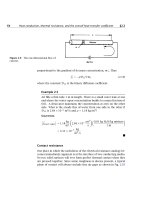
7.4 Heat transfer surface viewed as a heat exchanger
Let us reconsider the problem of a fluid flowing through a pipe with a
uniform wall temperature. By now we can predict
h for a pretty wide
range of conditions. Suppose that we need to know the net heat transfer
to a pipe of known length once
h is known. This problem is complicated
by the fact that the bulk temperature, T
b
, is varying along its length.
However, we need only recognize that such a section of pipe is a heat
exchanger whose overall heat transfer coefficient, U (between the wall
and the bulk), is just
h. Thus, if we wish to know how much pipe surface
area is needed to raise the bulk temperature from T
b
in
to T

b
out
, we can
calculate it as follows:
Q =
(
˙
mc
p
)
b

T
b
out
−T
b
in

= hA(LMTD)
or
A =
(
˙
mc
p
)
b

T

b
out
−T
b
in

h
ln

T
b
out
−T
w
T
b
in
−T
w


T
b
out
−T
w

−

T

b
in
−T
w

(7.56)
By the same token, heat transfer in a duct can be analyzed with the ef-
fectiveness method (Sect. 3.3) if the exiting fluid temperature is unknown.
368 Forced convection in a variety of configurations §7.4
Suppose that we do not know T
b
out
in the example above. Then we can
write an energy balance at any cross section, as we did in eqn. (7.8):
dQ = q
w
Pdx= hP
(
T
w
−T
b
)
dx =
˙
mc
P
dT
b
Integration can be done from T

b
(x = 0) = T
b
in
to T
b
(x = L) = T
b
out

L
0
hP
˙
mc
p
dx =−

T
b
out
T
b
in
d(T
w
−T
b
)
(T

w
−T
b
)
P
˙
mc
p

L
0
hdx =−ln

T
w
−T
b
out
T
w
−T
b
in

We recognize in this the definition of
h from eqn. (7.27). Hence,
hPL
˙
mc
p

=−ln

T
w
−T
b
out
T
w
−T
b
in

which can be rearranged as
T
b
out
−T
b
in
T
w
−T
b
in
= 1 − exp

−
hPL
˙

mc
p

(7.57)
This equation can be used in either laminar or turbulent flow to com-
pute the variation of bulk temperature if T
b
out
is replaced by T
b
(x), L is
replaced by x, and
h is adjusted accordingly.
The left-hand side of eqn. (7.57) is the heat exchanger effectiveness.
On the right-hand side we replace U with
h; we note that PL = A, the
exchanger surface area; and we write C
min
=
˙
mc
p
. Since T
w
is uniform,
the stream that it represents must have a very large capacity rate, so that
C
min
/C
max

= 0. Under these substitutions, we identify the argument of
the exponential as NTU = UA/C
min
, and eqn. (7.57) becomes
ε = 1 − exp
(
−NTU
)
(7.58)
which we could have obtained directly, from either eqn. (3.20)or(3.21),
by setting C
min
/C
max
= 0. A heat exchanger for which one stream is
isothermal, so that C
min
/C
max
= 0, is sometimes called a single-stream
heat exchanger.
Equation 7.57 applies to ducts of any cross-sectional shape. We can
cast it in terms of the hydraulic diameter, D
h
= 4A
c
/P, by substituting
§7.4 Heat transfer surface viewed as a heat exchanger 369
˙
m = ρu

av
A
c
:
T
b
out
−T
b
in
T
w
−T
b
in
= 1 − exp

−
hPL
ρu
av
c
p
A
c

= 1 − exp

−
h

ρu
av
c
p
4L
D
h

(7.59)
For a circular tube, with A
c
= πD
2
/4 and P = πD, D
h
= 4(πD
2
/4)

(πD)
= D. To use eqn. (7.59) for a noncircular duct, of course, we will need
the value of
h for its more complex geometry. We consider this issue in
the next section.
Example 7.5
Air at 20
◦
C is fully thermally developed as it flows ina1cmI.D. pipe.
The average velocity is 0.7m/s. If the pipe wall is at 60
◦

C , what is
the temperature 0.25 m farther downstream?
Solution.
Re
D
=
u
av
D
ν
=
(0.7)(0.01)
1.70 × 10
−5
= 412
The flow is therefore laminar, so
Nu
D
=
hD
k
= 3.658
Thus,
h =
3.658(0.0271)
0.01
= 9.91 W/m
2
K
Then

ε = 1 − exp

−
h
ρc
p
u
av
4L
D

= 1 − exp

−
9.91
1.14(1004)(0.7)
4(0.25)
0.01

so that
T
b
−20
60 − 20
= 0.698 or T
b
= 47.9
◦
C
370 Forced convection in a variety of configurations §7.5

7.5 Heat transfer coefficients for noncircular ducts
So far, we have focused on flows within circular tubes, which are by far the
most common configuration. Nevertheless, other cross-sectional shapes
often occur. For example, the fins of a heat exchanger may form a rect-
angular passage through which air flows. Sometimes, the passage cross-
section is very irregular, as might happen when fluid passes through a
clearance between other objects. In situations like these, all the qual-
itative ideas that we developed in Sections 7.1–7.3 still apply, but the
Nusselt numbers for circular tubes cannot be used in calculating heat
transfer rates.
The hydraulic diameter, which was introduced in connection with
eqn. (7.59), provides a basis for approximating heat transfer coefficients
in noncircular ducts. Recall that the hydraulic diameter is defined as
D
h
≡
4 A
c
P
(7.60)
where A
c
is the cross-sectional area and P is the passage’s wetted perime-
ter (Fig. 7.9). The hydraulic diameter measures the fluid area per unit
length of wall. In turbulent flow, where most of the convection resis-
tance is in the sublayer on the wall, this ratio determines the heat trans-
fer coefficient to within about ±20% across a broad range of duct shapes.
In fully-developed laminar flow, where the thermal resistance extends
into the core of the duct, the heat transfer coefficient depends on the
details of the duct shape, and D

h
alone cannot define the heat transfer
coefficient. Nevertheless, the hydraulic diameter provides an appropriate
characteristic length for cataloging laminar Nusselt numbers.
Figure 7.9 Flow in a noncircular duct.
§7.5 Heat transfer coefficients for noncircular ducts 371
The factor of four in the definition of D
h
ensures that it gives the
actual diameter of a circular tube. We noted in the preceding section
that, for a circular tube of diameter D, D
h
= D. Some other important
cases include:
a rectangular duct of
width a and height b
D
h
=
4 ab
2a + 2b
=
2ab
a + b
(7.61a)
an annular duct of
inner diameter D
i
and
outer diameter D

o
D
h
=
4

πD
2
o

4 − πD
2
i

4

π
(
D
o
+D
i
)
=
(
D
o
−D
i
)

(7.61b)
and, for very wide parallel plates, eqn. (7.61a) with a  b gives
two parallel plates
a distance b apart
D
h
= 2b (7.61c)
Turbulent flow in noncircular ducts
With some caution, we may use D
h
directly in place of the circular tube
diameter when calculating turbulent heat transfer coefficients and bulk
temperature changes. Specifically, D
h
replaces D in the Reynolds num-
ber, which is then used to calculate f and Nu
D
h
from the circular tube
formulas. The mass flow rate and the bulk velocity must be based on
the true cross-sectional area, which does not usually equal πD
2
h
/4 (see
Problem 7.46). The following example illustrates the procedure.
Example 7.6
An air duct carries chilled air at an inlet bulk temperature of T
b
in
=

17
◦
C and a speed of 1 m/s. The duct is made of thin galvanized steel,
has a square cross-section of 0.3 m by 0.3 m, and is not insulated.
A length of the duct 15 m long runs outdoors through warm air at
T
∞
= 37
◦
C. The heat transfer coefficient on the outside surface, due
to natural convection and thermal radiation, is 5 W/m
2
K. Find the
bulk temperature change of the air over this length.
Solution. The hydraulic diameter, from eqn. (7.61a) with a = b,is
simply
D
h
= a = 0.3m
372 Forced convection in a variety of configurations §7.5
Using properties of air at the inlet temperature (290 K), the Reynolds
number is
Re
D
h
=
u
av
D
h

ν
=
(1)(0.3)
(1.578 × 10
−5
)
= 19, 011
The Reynolds number for turbulent transition in a noncircular duct
is typically approximated by the circular tube value of about 2300, so
this flow is turbulent. The friction factor is obtained from eqn. (7.42)
f =

1.82 log
10
(19, 011) − 1.64

−2
= 0.02646
and the Nusselt number is found with Gnielinski’s equation, (7.43)
Nu
D
h
=
(0.02646/8)(19, 011 − 1, 000)(0.713)
1 + 12.7

0.02646/8

(0.713)
2/3

−1

= 49.82
The heat transfer coefficient is
h = Nu
D
h
k
D
h
=
(49.82)(0.02623)
0.3
= 4.371 W/m
2
K
The remaining problem is to find the bulk temperature change.
The thin metal duct wall offers little thermal resistance, but convec-
tion must be considered. Heat travels first from the air at T
∞
through
the outside heat transfer coefficient to the duct wall, and then through
the inside heat transfer coefficient to the flowing air — effectively
through two resistances in series from the fixed temperature T
∞
to
the rising temperature T
b
. We have seen in Section 2.4 that an overall
heat transfer coefficient may be used to describe such series resis-

tances. Here,
U =

1
h
inside
+
1
h
outside

−1
=

1
4.371
+
1
5

−1
= 2.332 W/m
2
K
We may then adapt eqn. (7.59) to our situation by replacing
h by U
and T
w
by T
∞

:
T
b
out
−T
b
in
T
∞
−T
b
in
= 1 − exp

−
U
ρu
av
c
p
4L
D
h

= 1 − exp

−
2.332
(1.217)(1)(1007)
4(15)

0.3

= 0.3165
The outlet bulk temperature is therefore
T
b
out
= [17 + (37 −17)(0.3165)]
◦
C = 23.3
◦
C
§7.5 Heat transfer coefficients for noncircular ducts 373
The accuracy of the procedure just outlined is generally within ±20%
and often within ±10%. Worse results are obtained for duct cross-sections
having sharp corners, such as an acute triangle. Specialized equations
for “effective” hydraulic diameters have been developed in the literature
and can improve the accuracy of predictions to 5 or 10% [7.8].
When only a portion of the duct cross-section is heated — one wall of
a rectangle, for example — the procedure is the same. The hydraulic di-
ameter is based upon the entire wetted perimeter, not simply the heated
part. One situation in which one-sided or unequal heating often occurs
is an annular duct, for which the inner tube might be a heating element.
The hydraulic diameter procedure will typically predict the heat transfer
coefficient on the outer tube to within ±10%, irrespective of the heating
configuration. The heat transfer coefficient on the inner surface, how-
ever, is sensitive to both the diameter ratio and the heating configuration.
For that surface, the hydraulic diameter approach is not very accurate,
especially if D
i

 D
o
; other methods have been developed to accurately
predict heat transfer in annular ducts. (see [7.3]or[7.8]).
Laminar flow in noncircular ducts
Laminar velocity profiles in noncircular ducts develop in essentially the
same way as for circular tubes, and the fully developed velocity profiles
are generally paraboloidal in shape. For example, for fully developed flow
between parallel plates located at y = b/2 and y =−b/2, the velocity
profile is
u
u
av
=
3
2

1 − 4

y
b

2

(7.62)
for u
av
the bulk velocity. This should be compared to eqn. (7.15) for a
circular tube. The constants and coordinates differ, but the equations
are otherwise identical. Likewise, an analysis of the temperature profiles

between parallel plates leads to constant Nusselt numbers, which may
be expressed in terms of the hydraulic diameter for various boundary
conditions:
Nu
D
h
=
hD
h
k
=







7.541 for fixed plate temperatures
8.235 for fixed flux at both plates
5.385 one plate fixed flux, one adiabatic
(7.63)
Some other cases are summarized in Table 7.4. Many more have been
considered in the literature (see, especially, [7.5]). The latter include
374 Forced convection in a variety of configurations §7.6
Table 7.4 Laminar, fully developed Nusselt numbers based on
hydraulic diameters given in eqn. (7.61)
Cross-section T
w
fixed q

w
fixed
Circular 3.657 4.364
Square 2.976 3.608
Rectangular
a = 2b 3.391 4.123
a = 4b 4.439 5.331
a = 8b 5.597 6.490
Parallel plates 7.541 8.235
different wall boundary conditions and a wide variety cross-sectional
shapes, both practical and ridiculous: triangles, circular sectors, trape-
zoids, rhomboids, hexagons, limaçons, and even crescent moons! The
boundary conditions, in particular, should be considered when the duct
is small (so that h will be large): if the conduction resistance of the tube
wall is comparable to the convective resistance within the duct, then tem-
perature or flux variations around the tube perimeter must be expected.
This will significantly affect the laminar Nusselt number. The rectangu-
lar duct values in Table 7.4 for fixed wall flux, for example, assume a
uniform temperature around the perimeter of the tube, as if the wall has
no conduction resistance around its perimeter. This might be true for a
copper duct heated at a fixed rate in watts per meter of duct length.
Laminar entry length formulæ for noncircular ducts are also given by
Shah and London [7.5].
7.6 Heat transfer during cross flow over cylinders
Fluid flow pattern
It will help us to understand the complexity of heat transfer from bodies
in a cross flow if we first look in detail at the fluid flow patterns that occur
in one cross-flow configuration—a cylinder with fluid flowing normal to
it. Figure 7.10 shows how the flow develops as Re ≡ u
∞

D/ν is increased
from below 5 to near 10
7
. An interesting feature of this evolving flow
pattern is the fairly continuous way in which one flow transition follows
§7.6 Heat transfer during cross flow over cylinders 375
Figure 7.10 Regimes of fluid flow across circular cylinders [7.22].
376 Forced convection in a variety of configurations §7.6
Figure 7.11 The Strouhal–Reynolds number relationship for
circular cylinders, as defined by existing data [7.22].
another. The flow field degenerates to greater and greater degrees of
disorder with each successive transition until, rather strangely, it regains
order at the highest values of Re
D
.
An important reflection of the complexity of the flow field is the
vortex-shedding frequency, f
v
. Dimensional analysis shows that a di-
mensionless frequency called the Strouhal number, Str, depends on the
Reynolds number of the flow:
Str ≡
f
v
D
u
∞
= fn
(
Re

D
)
(7.64)
Figure 7.11 defines this relationship experimentally on the basis of about
550 of the best data available (see [7.22]). The Strouhal numbers stay a
little over 0.2 over most of the range of Re
D
. This means that behind
a given object, the vortex-shedding frequency rises almost linearly with
velocity.
Experiment 7.1
When there is a gentle breeze blowing outdoors, go out and locate a
large tree with a straight trunk or the shaft of a water tower. Wet your
§7.6 Heat transfer during cross flow over cylinders 377
Figure 7.12 Giedt’s local measurements
of heat transfer around a cylinder in a
normal cross flow of air.
finger and place it in the wake a couple of diameters downstream and
about one radius off center. Estimate the vortex-shedding frequency and
use Str  0.21 to estimate u
∞
. Is your value of u
∞
reasonable?
Heat transfer
The action of vortex shedding greatly complicates the heat removal pro-
cess. Giedt’s data [7.23] in Fig. 7.12 show how the heat removal changes
as the constantly fluctuating motion of the fluid to the rear of the cylin-
378 Forced convection in a variety of configurations §7.6
der changes with Re

D
. Notice, for example, that Nu
D
is near its minimum
at 110
◦
when Re
D
= 71, 000, but it maximizes at the same place when
Re
D
= 140, 000. Direct prediction by the sort of b.l. methods that we
discussed in Chapter 6 is out of the question. However, a great deal can
be done with the data using relations of the form
Nu
D
= fn
(
Re
D
, Pr
)
The broad study of Churchill and Bernstein [7.24] probably brings
the correlation of heat transfer data from cylinders about as far as it is
possible. For the entire range of the available data, they offer
Nu
D
= 0.3 +
0.62 Re
1/2

D
Pr
1/3

1 + (0.4/Pr)
2/3

1/4

1 +

Re
D
282, 000

5/8

4/5
(7.65)
This expression underpredicts most of the data by about 20% in the range
20, 000 < Re
D
< 400, 000 but is quite good at other Reynolds numbers
above Pe
D
≡ Re
D
Pr = 0.2. This is evident in Fig. 7.13, where eqn. (7.65)
is compared with data.
Greater accuracy and, in most cases, greater convenience results from

breaking the correlation into component equations:
• Below Re
D
= 4000, the bracketed term [1 + (Re
D
/282, 000)
5/8
]
4/5
is  1, so
Nu
D
= 0.3 +
0.62 Re
1/2
D
Pr
1/3

1 + (0.4/Pr)
2/3

1/4
(7.66)
• Below Pe = 0.2, the Nakai-Okazaki [7.25] relation
Nu
D
=
1
0.8237 − ln


Pe
1/2

(7.67)
should be used.
• In the range 20, 000 < Re
D
< 400, 000, somewhat better results are
given by
Nu
D
= 0.3 +
0.62 Re
1/2
D
Pr
1/3

1 + (0.4/Pr)
2/3

1/4

1 +

Re
D
282, 000


1/2

(7.68)
than by eqn. (7.65).
§7.6 Heat transfer during cross flow over cylinders 379
Figure 7.13 Comparison of Churchill and Bernstein’s correla-
tion with data by many workers from several countries for heat
transfer during cross flow over a cylinder. (See [7.24] for data
sources.) Fluids include air, water, and sodium, with both q
w
and T
w
constant.
All properties in eqns. (7.65)to(7.68) are to be evaluated at a film tem-
perature T
f
= (T
w
+T
∞
)

2.
Example 7.7
An electric resistance wire heater 0.0001 m in diameter is placed per-
pendicular to an air flow. It holds a temperature of 40
◦
Cina20
◦
C air

flow while it dissipates 17.8W/m of heat to the flow. How fast is the
air flowing?
Solution.
h = (17.8W/m)

[π(0.0001 m)(40 − 20)K]= 2833
W/m
2
K. Therefore, Nu
D
= 2833(0.0001)/0.0264 = 10.75, where we
have evaluated k = 0.0264 at T = 30
◦
C. We now want to find the Re
D
for which Nu
D
is 10.75. From Fig. 7.13 we see that Re
D
is around 300
380 Forced convection in a variety of configurations §7.6
when the ordinate is on the order of 10. This means that we can solve
eqn. (7.66) to get an accurate value of Re
D
:
Re
D
=




(
Nu
D
−0.3)


1 +

0.4
Pr

2/3

1/4

0.62 Pr
1/3



2
but Pr = 0.71, so
Re
D
=



(10.75 − 0.3)



1 +

0.40
0.71

2/3

1/4

0.62(0.71)
1/3



2
= 463
Then
u
∞
=
ν
D
Re
D
=

1.596 × 10
−5

10
−4

463 = 73.9m/s
The data scatter in Re
D
is quite small—less than 10%, it would
appear—in Fig. 7.13. Therefore, this method can be used to measure
local velocities with good accuracy. If the device is calibrated, its
accuracy is improved further. Such an air speed indicator is called a
hot-wire anemometer, as discussed further in Problem 7.45.
Heat transfer during flow across tube bundles
A rod or tube bundle is an arrangement of parallel cylinders that heat, or
are being heated by, a fluid that might flow normal to them, parallel with
them, or at some angle in between. The flow of coolant through the fuel
elements of all nuclear reactors being used in this country is parallel to
the heating rods. The flow on the shell side of most shell-and-tube heat
exchangers is generally normal to the tube bundles.
Figure 7.14 shows the two basic configurations of a tube bundle in
a cross flow. In one, the tubes are in a line with the flow; in the other,
the tubes are staggered in alternating rows. For either of these configura-
tions, heat transfer data can be correlated reasonably well with power-law
relations of the form
Nu
D
= C Re
n
D
Pr
1/3

(7.69)
but in which the Reynolds number is based on the maximum velocity,
u
max
= u
av
in the narrowest transverse area of the passage
§7.6 Heat transfer during cross flow over cylinders 381
Figure 7.14 Aligned and staggered tube rows in tube bundles.
Thus, the Nusselt number based on the average heat transfer coefficient
over any particular isothermal tube is
Nu
D
=
hD
k
and Re
D
=
u
max
D
ν
Žukauskas at the Lithuanian Academy of Sciences Institute in Vilnius
has written two comprehensive review articles on tube-bundle heat trans-
382 Forced convection in a variety of configurations §7.6
fer [7.26, 7.27]. In these he summarizes his work and that of other Soviet
workers, together with earlier work from the West. He was able to corre-
late data over very large ranges of Pr, Re
D

, S
T
/D, and S
L
/D (see Fig. 7.14)
with an expression of the form
Nu
D
= Pr
0.36
(
Pr/Pr
w
)
n
fn
(
Re
D
)
with n =



0 for gases
1
4
for liquids
(7.70)
where properties are to be evaluated at the local fluid bulk temperature,

except for Pr
w
, which is evaluated at the uniform tube wall temperature,
T
w
.
The function fn(Re
D
) takes the following form for the various circum-
stances of flow and tube configuration:
100  Re
D
 10
3
:
aligned rows: fn
(
Re
D
)
= 0.52 Re
0.5
D
(7.71a)
staggered rows: fn
(
Re
D
)
= 0.71 Re

0.5
D
(7.71b)
10
3
 Re
D
 2 × 10
5
:
aligned rows: fn
(
Re
D
)
= 0.27 Re
0.63
D
,S
T
/S
L
 0.7
(7.71c)
For S
T
/S
L
< 0.7, heat exchange is much less effective.
Therefore, aligned tube bundles are not designed in this

range and no correlation is given.
staggered rows: fn
(
Re
D
)
= 0.35
(
S
T
/S
L
)
0.2
Re
0.6
D
,
S
T
/S
L
 2 (7.71d)
fn
(
Re
D
)
= 0.40 Re
0.6

D
,S
T
/S
L
> 2 (7.71e)
Re
D
> 2 × 10
5
:
aligned rows: fn
(
Re
D
)
= 0.033 Re
0.8
D
(7.71f)
staggered rows: fn
(
Re
D
)
= 0.031
(
S
T
/S

L
)
0.2
Re
0.8
D
,
Pr > 1 (7.71g)
Nu
D
= 0.027
(
S
T
/S
L
)
0.2
Re
0.8
D
,
Pr = 0.7 (7.71h)
All of the preceding relations apply to the inner rows of tube bundles.
The heat transfer coefficient is smaller in the rows at the front of a bundle,
§7.6 Heat transfer during cross flow over cylinders 383
Figure 7.15 Correction for the heat
transfer coefficients in the front rows of a
tube bundle [7.26].
facing the oncoming flow. The heat transfer coefficient can be corrected

so that it will apply to any of the front rows using Fig. 7.15.
Early in this chapter we alluded to the problem of predicting the heat
transfer coefficient during the flow of a fluid at an angle other than 90
◦
to the axes of the tubes in a bundle. Žukauskas provides the empirical
corrections in Fig. 7.16 to account for this problem.
The work of Žukauskas does not extend to liquid metals. However,
Kalish and Dwyer [7.28] present the results of an experimental study of
heat transfer to the liquid eutectic mixture of 77.2% potassium and 22.8%
sodium (called NaK). NaK is a fairly popular low-melting-point metallic
coolant which has received a good deal of attention for its potential use in
certain kinds of nuclear reactors. For isothermal tubes in an equilateral
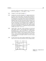
triangular array, as shown in Fig. 7.17, Kalish and Dwyer give
Nu
D
=

5.44 + 0.228 Pe
0.614





C
P −D
P

sin φ + sin
2

φ
1 + sin
2
φ

(7.72)
Figure 7.16 Correction for the heat
transfer coefficient in flows that are not
perfectly perpendicular to heat exchanger
tubes [7.26].
384 Forced convection in a variety of configurations §7.7
Figure 7.17 Geometric correction for
the Kalish-Dwyer equation (7.72).
where
• φ is the angle between the flow direction and the rod axis.
• P is the “pitch” of the tube array, as shown in Fig. 7.17, and D is
the tube diameter.
• C is the constant given in Fig. 7.17.
• Pe
D
is the Péclét number based on the mean flow velocity through
the narrowest opening between the tubes.
• For the same uniform heat flux around each tube, the constants in
eqn. (7.72) change as follows: 5.44 becomes 4.60; 0.228 becomes
0.193.
7.7 Other configurations
At the outset, we noted that this chapter would move further and further
beyond the reach of analysis in the heat convection problems that it dealt
with. However, we must not forget that even the most completely em-
pirical relations in Section 7.6 were devised by people who were keenly

aware of the theoretical framework into which these relations had to fit.
Notice, for example, that eqn. (7.66) reduces to Nu
D
∝

Pe
D
as Pr be-
comes small. That sort of theoretical requirement did not just pop out
of a data plot. Instead, it was a consideration that led the authors to
select an empirical equation that agreed with theory at low Pr.
Thus, the theoretical considerations in Chapter 6 guide us in correlat-
ing limited data in situations that cannot be analyzed. Such correlations
§7.7 Other configurations 385
can be found for all kinds of situations, but all must be viewed critically.
Many are based on limited data, and many incorporate systematic errors
of one kind or another.
In the face of a heat transfer situation that has to be predicted, one
can often find a correlation of data from similar systems. This might in-
volve flow in or across noncircular ducts; axial flow through tube or rod
bundles; flow over such bluff bodies as spheres, cubes, or cones; or flow
in circular and noncircular annuli. The Handbook of Heat Transfer [7.29],
the shelf of heat transfer texts in your library, or the journals referred
to by the Engineering Index are among the first places to look for a cor-
relation curve or equation. When you find a correlation, there are many
questions that you should ask yourself:
• Is my case included within the range of dimensionless parameters
upon which the correlation is based, or must I extrapolate to reach
my case?
• What geometric differences exist between the situation represented

in the correlation and the one I am dealing with? (Such elements as
these might differ:
(a) inlet flow conditions;
(b) small but important differences in hardware, mounting brack-
ets, and so on;
(c) minor aspect ratio or other geometric nonsimilarities
• Does the form of the correlating equation that represents the data,
if there is one, have any basis in theory? (If it is only a curve fit to
the existing data, one might be unjustified in using it for more than
interpolation of those data.)
• What nuisance variables might make our systems different? For
example:
(a) surface roughness;
(b) fluid purity;
(c) problems of surface wetting
• To what extend do the data scatter around the correlation line? Are
error limits reported? Can I actually see the data points? (In this
regard, you must notice whether you are looking at a correlation
386 Chapter 7: Forced convection in a variety of configurations
on linear or logarithmic coordinates. Errors usually appear smaller
than they really are on logarithmic coordinates. Compare, for ex-
ample, the data of Figs. 8.3 and 8.10.)
• Are the ranges of physical variables large enough to guarantee that
I can rely on the correlation for the full range of dimensionless
groups that it purports to embrace?
• Am I looking at a primary or secondary source (i.e., is this the au-
thor’s original presentation or someone’s report of the original)? If
it is a secondary source, have I been given enough information to
question it?
• Has the correlation been signed by the persons who formulated it?

(If not, why haven’t the authors taken responsibility for the work?)
Has it been subjected to critical review by independent experts in
the field?
Problems
7.1 Prove that in fully developed laminar pipe flow, (−dp/dx)R
2

4µ
is twice the average velocity in the pipe. To do this, set the
mass flow rate through the pipe equal to (ρu
av
)(area).
7.2 A flow of air at 27
◦
C and 1 atm is hydrodynamically fully de-
veloped ina1cmI.D. pipe with u
av
= 2m/s. Plot (to scale) T
w
,
q
w
, and T
b
as a function of the distance x after T
w
is changed
or q
w
is imposed:

a. In the case for which T
w
= 68.4
◦
C = constant.
b. In the case for which q
w
= 378 W/m
2
= constant.
Indicate x
e
t
on your graphs.
7.3 Prove that C
f
is 16/Re
D
in fully developed laminar pipe flow.
7.4 Air at 200
◦
C flows at 4 m/sovera3cmO.D. pipe that is kept
at 240
◦
C. (a) Find h. (b) If the flow were pressurized water at
200
◦
C, what velocities would give the same h, the same Nu
D
,

and the same Re
D
? (c) If someone asked if you could model
the water flow with an air experiment, how would you answer?
[u
∞
= 0.0156 m/s for same Nu
D
.]
Problems 387
7.5 Compare the h value calculated in Example 7.3 with those
calculated from the Dittus-Boelter, Colburn, and Sieder-Tate
equations. Comment on the comparison.
7.6 Water at T
b
local
= 10
◦
C flows ina3cmI.D. pipe at 1 m/s. The
pipe walls are kept at 70
◦
C and the flow is fully developed.
Evaluate h and the local value of dT
b
/dx at the point of inter-
est. The relative roughness is 0.001.
7.7 Water at 10
◦
C flows overa3cmO.D. cylinder at 70
◦

C. The
velocity is 1 m/s. Evaluate
h.
7.8 Consider the hot wire anemometer in Example 7.7. Suppose
that 17.8W/m is the constant heat input, and plot u
∞
vs. T
wire
over a reasonable range of variables. Must you deal with any
changes in the flow regime over the range of interest?
7.9 Water at 20
◦
C flows at 2 m/s over a 2 m length of pipe, 10 cm in
diameter, at 60
◦
C. Compare h for flow normal to the pipe with
that for flow parallel to the pipe. What does the comparison
suggest about baffling in a heat exchanger?
7.10 A thermally fully developed flow of NaK in a 5 cm I.D. pipe
moves at u
av
= 8m/s. If T
b
= 395
◦
C and T
w
is constant at
403
◦

C, what is the local heat transfer coefficient? Is the flow
laminar or turbulent?
7.11 Water entersa7cmI.D. pipe at 5
◦
C and moves through it at an
average speed of 0.86 m/s. The pipe wall is kept at 73
◦
C. Plot
T
b
against the position in the pipe until (T
w
− T
b
)/68 = 0.01.
Neglect the entry problem and consider property variations.
7.12 Air at 20
◦
C flows over a very large bank of 2 cm O.D. tubes
that are kept at 100
◦
C. The air approaches at an angle 15
◦
off
normal to the tubes. The tube array is staggered, with S
L
=
3.5cmandS
T
= 2.8 cm. Find h on the first tubes and on the

tubes deep in the array if the air velocity is 4.3m/s before it
enters the array. [
h
deep
= 118 W/m
2
K.]
7.13 Rework Problem 7.11 using a single value of
h evaluated at
3(73 − 5)/4 = 51
◦
C and treating the pipe as a heat exchan-
ger. At what length would you judge that the pipe is no longer
efficient as an exchanger? Explain.
388 Chapter 7: Forced convection in a variety of configurations
7.14 Go to the periodical engineering literature in your library. Find
a correlation of heat transfer data. Evaluate the applicability of
the correlation according to the criteria outlined in Section 7.7.
7.15 Water at 24
◦
C flows at 0.8m/s in a smooth, 1.5 cm I.D. tube
that is kept at 27
◦
C. The system is extremely clean and quiet,
and the flow stays laminar until a noisy air compressor is turned
on in the laboratory. Then it suddenly goes turbulent. Calcu-
late the ratio of the turbulent h to the laminar h.[h
turb
=
4429 W/m

2
K.]
7.16 Laboratory observations of heat transfer during the forced flow
of air at 27
◦
C over a bluff body, 12 cm wide, kept at 77
◦
C yield
q = 646 W/m
2
when the air moves 2 m/s and q = 3590 W/m
2
when it moves 18 m/s. In another test, everything else is the
same, but now 17
◦
C water flowing 0.4m/s yields 131,000 W/m
2
.
The correlations in Chapter 7 suggest that, with such limited
data, we can probably create a fairly good correlation in the
form:
Nu
L
= CRe
a
Pr
b
. Estimate the constants C, a, and b by
cross-plotting the data on log-log paper.
7.17 Air at 200 psia flows at 12 m/s in an 11 cm I.D. duct. Its bulk

temperature is 40
◦
C and the pipe wall is at 268
◦
C. Evaluate h
if ε/D = 0.00006.
7.18 How does
h during cross flow over a cylindrical heat vary with
the diameter when Re
D
is very large?
7.19 Air enters a 0.8 cm I.D. tube at 20
◦
C with an average velocity
of 0.8m/s. The tube wall is kept at 40
◦
C. Plot T
b
(x) until it
reaches 39
◦
C. Use properties evaluated at [(20 +40)/2]
◦
C for
the whole problem, but report the local error in h at the end
to get a sense of the error incurred by the simplification.
7.20 Write Re
D
in terms of
˙

m in pipe flow and explain why this rep-
resentation could be particularly useful in dealing with com-
pressible pipe flows.
7.21 NaK at 394
◦
C flows at 0.57 m/s across a 1.82 m length of
0.036 m O.D. tube. The tube is kept at 404
◦
C. Find h and the
heat removal rate from the tube.
7.22 Verify the value of h specified in Problem 3.22.