Beginning C# 2008 Databases From Novice to Professional phần 2 ppsx

Figure 2-10. SSMSE Object Explorer and Summary tabbed pane
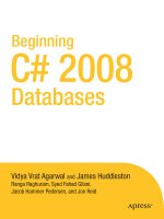
3. Expand the System Databases node, and your screen should resemble that shown
in Figure 2-11. As you can see, SSMS has four system databases:
• The
master database is the main controlling database, and it records all the
global information that is required for the SQL Server instance.
• The
model database works as a template for new databases to be created; in
other words, settings of the model database will be applied to all user-created
databases.
•
The
msdb database is used b
y SQL Server Agent for scheduling jobs and alerts.
• The
tempdb database holds temporary tables and other temporary database
objects, either generated automatically by SQL Server or created explicitly by
you. The temporary database is re-created each time the SQL Server instance
is started, so objects in it do not persist after SQL Server is shut down.
CHAPTER 2 ■ GETTING TO KNOW YOUR TOOLS 23
9004ch02final.qxd 12/13/07 4:22 PM Page 23
Figure 2-11. System databases
4. Click the AdventureWorks node in Object Explorer, and then click New Query to
bring up a new SQL edit window, as shown in Figure 2-12. As mentioned in Chap-
ter 1, AdventureWorks is a new sample database introduced for the first time with
SQL Server 2005.
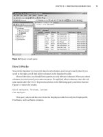
5. To see a listing of the tables residing inside AdventureWorks, type the query select
name from sysobjects where xtype=‘U’
and click the Execute button. The table
names will appear in the Results tab (see F
igure 2-12). If you navigate to the Mes-

sages tab, you will see the message “70 row(s) affected,” which means that the
AdventureWorks database consists of 70 tables.
6. Click File ➤ Disconnect Object Explorer.
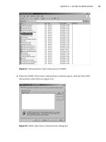
7. Click the N
or
thwind node in Object E
xplor
er
, and then click New Query. To see
the table names r
esiding inside N
or
thwind, type the quer
y
select name fr
om sys
-
objects wher
e xtype=‘U’
and click the E
xecute button. A listing of tables in the
database will appear in the R
esults tab (see F
igur
e 2-13). I
f you navigate to the
M
essages tab
, y
ou will see the message

“13 row(s) affected,” which means that
the N
or
thwind database consists of 13 tables
.
8. Click F
ile
➤ D
isconnect Object Explorer, and then close SQL Server Management
S
tudio Express.
CHAPTER 2 ■ GETTING TO KNOW YOUR TOOLS24
9004ch02final.qxd 12/13/07 4:22 PM Page 24
Figure 2-12. Tables in the AdventureWorks database
Figure 2-13. Tables in the Northwind database
CHAPTER 2 ■ GETTING TO KNOW YOUR TOOLS 25
9004ch02final.qxd 12/13/07 4:22 PM Page 25
Summary
In this chapter, we covered just enough about Visual Studio 2008 and SQL Server Man-
agement Studio to get you familiar with the kinds of things you’ll do with these tools later
in this book. Besides these tools, we also covered a bit about multiple .NET Framework
versions on a single system.
Now that your tools are installed and configured, you can start learning how to do
database programming by learning the basics of T-SQL.
CHAPTER 2 ■ GETTING TO KNOW YOUR TOOLS26
9004ch02final.qxd 12/13/07 4:22 PM Page 26
Getting to Know
Relational Databases
Now that you have gotten to know the tools you’ll use in this book, we’ll step back a bit
to give you a brief introduction to the important concepts of the PC database world

before diving into the examples.
In this chapter, we’ll cover the following:
• What is a database?
• Choosing between a spreadsheet and a database
• Why use a database?
• Benefits of using a relational database management system
• Comparing desktop and server RDBMS systems
• The database life cy
cle
• Mapping cardinalities
• Understanding keys
• Understanding data integrity
• Normalization concepts
• Drawbacks of normalization
What Is a Database?
In very simple terms, a database is a collection of structured information. Databases are
designed specifically to manage large bodies of information, and they store data in an
27
CHAPTER 3
9004ch03final.qxd 12/13/07 4:21 PM Page 27
organized and structured manner that makes it easy for users to manage and retrieve
that data when required.
A
database management system (DBMS) is a software program that enables users to
create and maintain databases. A DBMS also allows users to write queries for an individ-
ual database to perform required actions like retrieving data, modifying data, deleting
data, and so forth.
DBMSs support
tables (a.k.a. relations or entities) to store data in rows (a.k.a. records
or tuples) and columns (a.k.a. fields or attributes), similar to how data appears in a

spreadsheet application.
A
relational database management system, or RDBMS, is a type of DBMS that stores
information in the form of related tables. RDBMS is based on the
relational model.
Choosing Between a Spreadsheet and a Database
If databases are much like spreadsheets, why do people still use database applications? A
database is designed to perform the following actions in an easier and more productive
manner than a spreadsheet application would require:
• Retrieve all records that match particular criteria.
• Update or modify a complete set of records at one time.
• Extract values from records distributed among multiple tables.
Why Use a Database?
Following are some of the reasons w
e use databases:
•
Compactness: Databases help in maintaining large amounts of data, and thus com-
pletely replace voluminous paper files.
•
S
peed
:
S
earches for a particular piece of data or information in a database are
much faster than sor
ting through piles of paper.
•
Less drudgery: It is a dull work to maintain files by hand; using a database com-
pletely eliminates such maintenance.
•

Currency: Database systems can easily be updated and so provide accurate infor-
mation all the time and on demand.
CHAPTER 3 ■ GETTING TO KNOW RELATIONAL DATABASES28
9004ch03final.qxd 12/13/07 4:21 PM Page 28
Benefits of Using a Relational Database
Management System
RDBMSs offer various benefits by controlling the following:
•
Redundancy: RDBMSs prevent having multiple duplicate copies of the same data,
which takes up disk space unnecessarily.
•
Inconsistency: Each redundant set of data may no longer agree with other sets of
the same data. When an RDBMS removes redundancy, inconsistency cannot occur.
•
Data integrity: Data values stored in the database must satisfy certain types of con-
sistency constraints. (We’ll discuss this benefit in more detail in the section
“Understanding Data Integrity” later in this chapter.)
•
Data atomicity: In event of a failure, data is restored to the consistent state it
existed in prior to the failure. For example, fund transfer activity must be atomic.
(We cover the fund transfer activity and atomicity in more detail in Chapter 8.)
•
Access anomalies: RDBMSs prevent more than one user from updating the same
data simultaneously; such concurrent updates may result in inconsistent data.
•
Data security: Not every user of the database system should be able to access all
the data. Security refers to the protection of data against any unauthorized access.
•
Transaction processing: A transaction is a sequence of database operations that
represents a logical unit of work. In RDBMSs, a transaction either commits all the

changes or rolls back all the actions performed till the point at which failure
occurred.
•
Recovery: Recovery features ensure that data is reorganized into a consistent state
after a transaction fails.
•
Storage management: RDBMSs provide a mechanism for data storage manage-
ment. The internal schema defines how data should be stored.
Comparing Desktop and Server RDBMS Systems
In the industry today, we mainly work with two types of databases: desktop databases
and server databases. Here, we’ll give you a brief look at each of them.
CHAPTER 3 ■ GETTING TO KNOW RELATIONAL DATABASES 29
9004ch03final.qxd 12/13/07 4:21 PM Page 29
Desktop Databases
Desktop databases are designed to serve a limited number of users and run on desktop
PCs, and they offer a less-expansive solution wherever a database is required. Chances
are you have worked with a desktop database program—Microsoft SQL Server Express,
Microsoft Access, Microsoft FoxPro, FileMaker Pro, Paradox, and Lotus represent a wide
range of desktop database solutions.
Desktop databases differ from server databases in the following ways:
•
Less expensive: Most desktop solutions are available for just a few hundred dollars.
In fact, if you own a licensed version of Microsoft Office Professional, you’re
already a licensed owner of Microsoft Access, which is one of the most commonly
and widely used desktop database programs around.
•
User friendly: Desktop databases are quite user friendly and easy to work with,
as they do not require complex SQL queries to perform database operations
(although some desktop databases also support SQL syntax if you would like to
code). Desktop databases generally offer an easy-to-use graphical user interface.

Server Databases
Server databases are specifically designed to serve multiple users at a time and offer fea-
tures that allow you to manage large amounts of data very efficiently by serving multiple
user requests simultaneously. Well-known examples of server databases include
Microsoft SQL Server, Oracle, Sybase, and DB2.
Following are some other char
acteristics that differentiate server databases from
their desktop counterparts:
•
Flexibility: Server databases are designed to be very flexible to support multiple
platforms, respond to requests coming from multiple database users, and perform
any database management task with optimum speed.
• Availability: Server databases are intended for enterprises, and so they need to be
available 24/7. To be available all the time, server databases come with some high-
availability features, such as mirroring and log shipping.
•
P
er
formance
:
S
er
v
er databases usually hav
e huge hardware support, and so servers
r
unning these databases hav
e lar
ge amounts of RAM and multiple CPU
s

, and this
is why ser
v
er databases suppor
t r
ich infr
astructure and give optimum perform-
ance
.
•
Scalability: This property allows a server database to expand its ability to process
and store records even if it has grown tremendously.
CHAPTER 3 ■ GETTING TO KNOW RELATIONAL DATABASES30
9004ch03final.qxd 12/13/07 4:21 PM Page 30
The Database Life Cycle
The database life cycle defines the complete process from conception to implementa-
tion. The entire development and implementation process of this cycle can be divided
into small phases; only after the completion of each phase can you move on to the next
phase, and this is the way you build your database block by block.
Before getting into the development of any system, you need to have strong a life-
cycle model to follow. The model must have all the phases defined in proper sequence,
which will help the development team to build the system with fewer problems and full
functionality as expected.
The database life cycle consists of the following stages, from the basic steps
involved in designing a global schema of the database to database implementation
and maintenance:
•
Requirement analysis: Requirements need to be determined before you can begin
design and implementation. The requirements can be gathered by interviewing
both the producer and the user of the data; this process helps in creating a formal

requirement specification.
•
Logical design: After requirement gathering, data and relationships need to be
defined using a conceptual data modeling technique such as an entity relationship
(ER) diagram.
•
Physical design: Once the logical design is in place, the next step is to produce the
physical structure for the database. The physical design phase involves table cre-
ation and selection of indexes.
•
Database implementation: Once the design is completed, the database can be cre-
ated thr
ough implementation of formal schema using the data definition language
(DDL) of the RDBMS.
•
Data modification: Data modification language (DML) can be used to query and
update the database as well as set up indexes and establish constraints such as ref-
erential integrity.
•
D
atabase
monitoring
: As the database begins oper
ation, monitor
ing indicates
whether per
for
mance r
equir
ements are being met; if they are not, modifications

should be made to impr
o
v
e database performance. Thus the database life cycle
continues with monitor
ing, r
edesign, and modification.
CHAPTER 3 ■ GETTING TO KNOW RELATIONAL DATABASES 31
9004ch03final.qxd 12/13/07 4:21 PM Page 31
Mapping Cardinalities
Tables are the fundamental components of a relational database. In fact, both data and
relationships are stored simply as data in tables.
Tables are composed of rows and columns. Each column represents a piece of
information.
Mapping cardinalities, or cardinality ratios, express the number of entities to which
another entity can be associated via a relationship set.
Cardinality refers to the unique-
ness of data values contained in a particular column of a database table. The term
relational database refers to the fact that different tables quite often contain related data.
For example, one sales rep in a company may take many orders, which were placed by
many customers. The products ordered may come from different suppliers, and chances
are that each supplier can supply more than one product. All of these relationships exist
in almost every database and can be classified as follows:
One-to-One (1:1) For each row in Table A, there is at most only one related row in Table B,
and vice versa. This relationship is typically used to separate data by frequency of use to
optimally organize data physically. For example, one department can have only one
department head.
One-to-Many (1:M) For each row in Table A, there can be zero or more related rows in
Table B; but for each row in Table B, there is at most one row in Table A. This is the most
common relationship. An example of a one-to-many relationship of tables in Northwind

is shown in Figure 3-1. Note the Customers table has a CustomerID field as the
primary
key
(indicated by the key symbol on the left), which has a relation with the CustomerID
field of the Orders table; C
ustomerID is considered a
foreign key in the Orders table
. The
link shown between the Customers and Orders tables indicates a one-to-many r
elation-
ship, as many orders can belong to one customer. Here, Customers is referred to as the
parent table, and Orders is the child table in the relationship.
CHAPTER 3 ■ GETTING TO KNOW RELATIONAL DATABASES32
9004ch03final.qxd 12/13/07 4:21 PM Page 32
Figure 3-1. A one-to-many relationship
Many-to-Man
y (M:M)
For each
row in Table A, there are zero or more related rows in
T
able B, and vice versa. Many-to-many relationships are not so easy to achieve, and
they r
equir
e a special technique to implement them.
This r
elationship is actually
implemented in a one-many
-one for
mat, so it r
equir

es a third table (often referred to
as a
junction table) to be intr
oduced in betw
een that ser
v
es as the path between the
r
elated tables
.
This is a v
er
y common r
elationship
. An example from Northwind is shown in Fig-
ur
e 3-2: an or
der can hav
e many pr
oducts and a product can belong to many orders.
The Or
der D
etails table not only r
epr
esents the M:M relationship, but also contains
data about each par
ticular or
der
-pr
oduct combination.

CHAPTER 3 ■ GETTING TO KNOW RELATIONAL DATABASES 33
9004ch03final.qxd 12/13/07 4:21 PM Page 33
Figure 3-2. A many-to-many relationship
■Note Though relationships among tables are extremely important, the term relational database has
nothing to do with them. Relational databases are (to varying extents) based on the
relational model of data
invented by Dr. Edgar F. Codd at IBM in the 1970s. Codd based his model on the mathematical (set-
theoretic) concept of a
relation. Relations are sets of tuples that can be manipulated with a well-defined
and well-behaved set of mathematical operations—in fact, two sets:
relational algebra and relational cal-
culus
. You don’t have to know or understand the mathematics to work with relational databases, but if you
hear it said that a database is relational because it “relates data,” you’ll know that whoever said it doesn’t
understand rela
tional da
tabases.
Understanding Keys
The key, the whole key, and nothing but the key, so help me Codd.
Relationships are represented by data in tables. To establish a relationship between two
tables, you need to have data in one table that enables you to find related rows in another
CHAPTER 3 ■ GETTING TO KNOW RELATIONAL DATABASES34
9004ch03final.qxd 12/13/07 4:21 PM Page 34
table. That’s where keys come in, and RDBMS mainly works with two types of keys, as
mentioned earlier: primary keys and foreign keys.
A key is one or more columns of a relation that is used to identify a row.
Primary Keys
A primary key is an attribute (column) or combination of attributes (columns) whose val-
ues uniquely identify records in an entity.
Before you choose a primary key for an entity, an attribute must have the following

properties:
• Each record of the entity must have a not-null value.
• The value must be unique for each record entered into the entity.
• The values must not change or become null during the life of each entity instance.
• There can be only one primary key defined for an entity.
Besides helping in uniquely identifying a record, the primary key also helps in
searching records as an index automatically gets generated as you assign a primary key
to an attribute.
An entity will have more than one attribute that can serve as a primary key. Any key
or minimum set of keys that could be a primary key is called a
candidate key. Once candi-
date keys are identified, choose one, and only one, primary key for each entity.
Sometimes it requires more than one attribute to uniquely identify an entity. A
pri-
mary key
that consists of more than one attribute is known as a composite key. There can
be only one
primary key in an entity, but a composite key can have multiple attributes
(i.e., a
primary key will be defined only once, but it can have up to 16 attributes). The pri-
mary key represents the parent entity. Primary keys are usually defined with the
IDENTITY
property, which allows insertion of an auto-incremented integer value into the table
when you insert a row into the table.
For
eign K
eys
A foreign key is an attribute that completes a relationship by identifying the parent entity.
Foreign keys provide a method for maintaining integrity in the data (called
referential

integrity
) and for navigating between different instances of an entity. Every relationship
in the model must be supported by a foreign key. For example, in Figure 3-1 earlier, the
Customers and Orders tables have a primary key and foreign key relationship, where the
Orders table’s CustomerID field is the foreign key having a reference to the CustomerID
field, which is the primary key of the Customers table.
CHAPTER 3 ■ GETTING TO KNOW RELATIONAL DATABASES 35
9004ch03final.qxd 12/13/07 4:21 PM Page 35
Understanding Data Integrity
Data integrity means that data values in a database are correct and consistent. There are
two aspects to data integrity:
entity integrity and referential integrity.
Entity Integrity
We mentioned previously in “Primary Keys” that no part of a primary key can be null.
This is to guarantee that primary key values exist for all rows. The requirement that pri-
mary key values exist and that they are unique is known as
entity integrity (EI). The DBMS
enforces
entity integrity by not allowing operations (INSERT, UPDATE) to produce an invalid
primary key. Any operation that creates a duplicate primary key or one containing nulls
is rejected. That is, to establish entity integrity, you need to define primary keys so the
DBMS can enfor
ce their uniqueness.
Referential Integrity
Once a relationship is defined between tables with foreign keys, the key data must be
managed to maintain the correct relationships, that is, to enforce
referential integrity
(RI). RI requires that all foreign key values in a child table either match primary key val-
ues in a parent table or (if permitted) be null. This is also known as satisfying a
foreign

key constraint
.
Normalization Concepts
Normalization is a technique for avoiding potential update anomalies, basically by mini-
mizing redundant data in a logical database design. N
ormalized designs are in a sense
“better” designs because they (ideally) keep each data item in only one place
. Normal-
iz
ed database designs usually r
educe update processing costs but can make query
processing more complicated. These trade-offs must be carefully evaluated in terms of
the required performance profile of a database. Often, a database design needs to be
denormalized to adequately meet operational needs.
Normalizing a logical database design involves a set of formal processes to sepa-
rate the data into multiple, related tables. The result of each process is referred to as a
normal form. Five normal forms have been identified in theory, but most of the time
third normal form (3NF) is as far as you need to go in practice. To be in 3NF, a
relation
(the formal term for what SQL calls a table and the precise concept on which the math-
ematical theory of normalization rests) must already be in second normal form (2NF),
and 2NF requires a relation to be in first normal form (1NF). Let’s look briefly at what
these normal forms mean.
CHAPTER 3 ■ GETTING TO KNOW RELATIONAL DATABASES36
9004ch03final.qxd 12/13/07 4:21 PM Page 36
First Normal Form (1NF) In first normal form, all column values are scalar; in other words,
they have a single value that can’t be further decomposed in terms of the data model. For
example, although individual characters of a string can be accessed through a procedure
that decomposes the string, only the full string is accessible
by name in SQL, so, as far as

the data model is concerned, they aren’t part of the model. Likewise, for a Managers table
with a manager column and a column containing a list of employees in Employees table
who work for a given manager, the manager and the list would be accessible by name,
but the individual employees in the list wouldn’t be. All relations—and SQL tables—are
by definition in 1NF since the lowest level of accessibility (known as the table’s
gran-
ularity
) is the column level, and column values are scalars in SQL.
Second Normal Form (2NF) Second normal form requires that attributes (the formal
term for SQL columns) that aren’t parts of keys be
functionally dependent on a key that
uniquely identifies them. Functional dependence basically means that for a given key
value, only one value exists in a table for a column or set of columns. For example, if a
table contained employees and their titles, and more than one employee could have
the same title (very likely), a key that uniquely identified employees wouldn’t uniquely
identify titles, so the titles wouldn’t be functionally dependent on a key of the table. To
put the table into 2NF, you’d create a separate table for titles—with its own unique
key—and replace the title in the original table with a foreign key to the new table. Note
how this reduces data redundancy. The titles themselves now appear only once in the
database. Only their keys appear in other tables, and key data isn’t considered redun-
dant (though, of course, it requires columns in other tables and data storage).
Third Normal Form (3NF) Thir
d normal form extends the concept of functional depend-
ence to
full functional dependence. Essentially, this means that all nonkey columns in a
table are uniquely identified by the whole
, not just part of, the primary key. For example,
if you revised the hypothetical 1NF Managers-Employees table to have three columns
(M
anagerName, EmployeeId, and EmployeeName) instead of two, and you defined the

composite primary key as ManagerName + EmployeeId, the table would be in 2NF (since
EmployeeName, the nonkey column, is dependent on the primary key), but it wouldn’t
be in 3NF (since EmployeeName is uniquely identified by part of the primary key defined
as column named EmployeeId). Creating a separate table for employees and removing
EmployeeName from Managers-Employees would put the table into 3NF. Note that even
though this table is now normalized to 3NF, the database design is still not as normalized
as it should be. Creating another table for managers using an ID shorter than the man-
ager’s name, though not required for normalization here, is definitely a better approach
and is probably advisable for a real-world database.
CHAPTER 3 ■ GETTING TO KNOW RELATIONAL DATABASES 37
9004ch03final.qxd 12/13/07 4:21 PM Page 37
Drawbacks of Normalization
Database design is an art more than a technology, and applying normalization wisely is
always important. On the other hand, normalization inherently increases the number of
tables and therefore the number of operations (called
joins) required to retrieve data.
Because data is not in one table, queries that have a complex join can slow things down.
This can cost in the form of CPU usage: the more complex the queries, the more CPU
time is required.
Denormalizing one or more tables, by intentionally providing redundant data to
reduce the number or complexity of joins to get quicker query response times, may be
necessary. With either normalization or denormalization, the goal is to control redun-
dancy so that the database design adequately (and ideally, optimally) supports the
actual use of the database.
Summary
This chapter has described basic database concepts. You also learned about desktop
and server databases, the stages of the database life cycle, and the types of keys and
how they define relationships. You also looked at normalization forms for designing a
better database.
In the next chapter, you’ll start working with database queries.

CHAPTER 3 ■ GETTING TO KNOW RELATIONAL DATABASES38
9004ch03final.qxd 12/13/07 4:21 PM Page 38
Writing Database Queries
In this chapter, you will learn about coding queries in SQL Server 2005. SQL Server
uses T-SQL as its language, and it has a wide variety of functions and constructs for
querying. Besides this, you will also be exploring new T-SQL features of SQL Server
2005 in this chapter. You will see how to use SQL Server Management Studio Express
and the AdventureWorks and Northwind databases to submit queries.
In this chapter, we’ll cover the following:
• Comparing QBE and SQL
• SQL Server Management Studio Express
• Beginning with queries
• Common table expressions
•
GROUP BY clause
•
PIVOT operator
•
ROW_NUMBER() function
•
PARTITION BY clause
• Pattern matching
•
Aggr
egate
functions
•
DATETIME functions
•
J

oins
39
CHAPTER 4
9004ch04final.qxd 12/13/07 4:19 PM Page 39
Comparing QBE and SQL
There are two main languages that have emerged for RDBMS—QBE and SQL.
Query by Example (QBE) is an alternative, graphical-based, point-and-click way of
querying a database. QBE was invented by Moshé M. Zloof at IBM Research during the
mid-1970s, in parallel to the development of SQL. It differs from SQL in that it has a
graphical user interface that allows users to write queries by creating example tables on
the screen. QBE is especially suited for queries that are not too complex and can be
expressed in terms of a few tables.
QBE was developed at IBM and is therefore an IBM trademark, but a number of other
companies also deal with query interfaces like QBE. Some systems, such as Microsoft
Access, have been influenced by QBE and have partial support for form-based queries.
Structured Query Language (SQL) is the standard relational database query lan-
guage. In the 1970s, a group at IBM’s San Jose Research Center (now the Almaden
Research Center) developed a database system named
System R based upon Codd’s
model. To manipulate and retrieve data stored in System R, a language called
Structured
English Q
uery Language
(SEQUEL) was designed.
Donald D. Chamberlin and Raymond F.
Boyce at IBM were the authors of the SEQUEL language design. The acronym SEQUEL
was later condensed to SQL. SQL was adopted as a standard by the American National
Standards Institute (ANSI) in 1986 and then ratified by International Organization for
Standardization (ISO) in 1987; this SQL standard was published as SQL 86 or SQL 1. Since
then, the SQL standar

ds have gone through many revisions. After SQL 86, there was SQL
89 (which included a minor revision); SQL 92, also known as SQL 2 (which was a major
revision); and then SQL 99, also known as SQL 3 (which added object-oriented features
that together represent the origination of the concept of ORDBMS, or object relational
database management system).
Each database vendor offers its own implementation of SQL that conforms at some
level to the standard but typically extends it. T-SQL does just that, and some of the SQL
used in this book may not work if you try it with a database server other than SQL Server.
■T
ip
Rela
tional da
tabase terminolog
y is often confusing.
For example, neither the meaning nor the pro-
nunciation of SQL is crystal clear. IBM invented the language back in the 1970s and called it SEQUEL,
changing it shortly thereafter to Structured Query Language SQL to avoid conflict with another vendor’s
product. SEQUEL and SQL were both pronounced “sequel.” When the ISO/ANSI standard was adopted, it
referred to the language simply as “database language SQL” and was silent on whether this was an acronym
and how it should be pronounced. Today, two pronunciations are used. In the Microsoft and Oracle worlds
(as well as many others), it’s pronounced “sequel.” In the DB2 and MySQL worlds (among others), it’s pro-
nounced “ess cue ell.” We’ll follow the most reasonable practice. We’re working in a Microsoft environment,
so we’ll go with “sequel” as the pronunciation of SQL.
CHAPTER 4 ■ WRITING DATABASE QUERIES40
9004ch04final.qxd 12/13/07 4:19 PM Page 40
Beginning with Queries
A query is a technique to extract information from a database. You need a query window
into which to type your query and run it so data can be retrieved from the database.
■Note Many of the examples from this point forward require you to work in SQL Server Management
Studio Express. Refer back to “Using SQL Server Management Studio Express” in Chapter 2 for instructions

if you need to refresh your memory on how to connect to SSMSE.
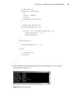
Try It Out: Running a Simple Query
1. Open SQL Server Management Studio Express, expand the Databases node, and
select the AdventureWorks database.
2. Click the New Query button in the top-left corner of the window, as shown in
Figure 4-1, and then enter the following query:
Select * from Sales.SalesReason
Figure 4-1. Writing a query
CHAPTER 4 ■ WRITING DATABASE QUERIES 41
9004ch04final.qxd 12/13/07 4:19 PM Page 41
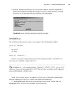
3. Click Execute (or press F5 or select Query ➤ Execute), and you should see the out-
put shown in the Results window as in Figure 4-2.
Figure 4-2. Query Results window
How It Works
Here, you use the asterisk (*) with the SELECT statement. The asterisk indicates that all the
columns from the specified table should be retrieved.
Common Table Expressions
Common table expressions (CTEs) are new to SQL Server 2005. A CTE is a named tem-
porary result set that will be used by the
FROM clause of a SELECT query. You then use the
result set in any
SELECT, INSERT, UPDATE, or DELETE query defined within the same scope as
the CTE.
The main advantage CTEs provide you is that the queries with derived tables become
simpler, as traditional Transact-SQL constructs used to work with derived tables usually
require a separate definition for the derived data (such as a temporary table). Using a
CTE to define the derived table makes it easier to see the definition of the derived table
with the code that uses it.
CHAPTER 4 ■ WRITING DATABASE QUERIES42
9004ch04final.qxd 12/13/07 4:19 PM Page 42

A CTE consists of three main elements:
• Name of the CTE followed by the
WITH keyword
• The column list (optional)
• The query that will appear within parentheses,
( ), after the AS keyword
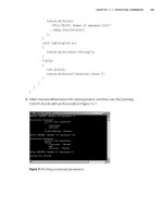
Try It Out: Creating a CTE
To create a CTE, enter the following query into SQL Server Management Studio Express
and execute it. You should see the results shown in Figure 4-3.
WITH TopSales (SalesPersonID,TerritoryID,NumberOfSales)
AS
(
SELECT SalesPersonID,TerritoryID, Count(*)
FROM Sales.SalesOrderHeader
GROUP BY SalesPersonID, TerritoryID
)
SELECT * FROM TopSales
WHERE SalesPersonID IS NOT NULL
ORDER BY NumberOfSales DESC
Figure 4-3. U
sing a common table e
xpr
ession
CHAPTER 4 ■ WRITING DATABASE QUERIES 43
9004ch04final.qxd 12/13/07 4:19 PM Page 43
How It Works
The CTE definition line in which you specify the CTE name and column list:
WITH TopSales (SalesPersonID,TerritoryID,NumberOfSales)
consists of three columns, which means that this SELECT statement:
SELECT SalesPersonID,TerritoryID, Count(*)

will also have three columns, and the individual column specified in the SELECT list will
map to the columns specified inside the CTE definition.
By running the CTE, you will see the SalesPersonID, TerritoryID, and NumberOfSales
made in that particular territory by a particular salesperson.
GROUP BY Clause
The GROUP BY clause is used to organize output rows into groups. The SELECT list can
include aggregate functions and produce summary values for each group. Often you’ll
want to generate reports from the database with summary figures for a particular column
or set of columns. For example, you may want to find out the total quantity of each card
type that expires in a specific year from the Sales.CreditCard table.
Try It Out: Using the GROUP BY Clause
The Sales.CreditCard table contains the details of credit cards. You need to total the cards
of a specific type that will be expiring in a particular year.
Open a New Query window in SQL Server Management Studio Express. Enter the fol-
lowing query and click Execute. You should see the results shown in Figure 4-4.
Use AdventureWorks
Go
Select CardType, ExpYear,count(CardType) AS 'Total Cards'
from Sales.CreditCard
Where ExpYear in (2006,2007)
group by ExpYear,CardType
order by CardType,ExpYear
CHAPTER 4 ■ WRITING DATABASE QUERIES44
9004ch04final.qxd 12/13/07 4:19 PM Page 44
Figure 4-4 Using GROUP BY to aggregate values
How It Works
You specify three columns and use the COUNT function to count the total number of cards
listed in the CardType column of the CreditCard table.
Select CardType, ExpYear,count(CardType) AS 'Total Cards'
from Sales.CreditCard

Then you specify the WHERE condition, and the GROUP BY and ORDER BY clauses. The
WHERE condition ensur
es that the car
ds listed will be those that will expir
e in either 2006
or
2007.
Where ExpYear in (2006,2007)
The GROUP BY clause enforces the grouping on the specified columns that the results
should be displayed in the form of groups for ExpYear and CardType columns.
group by ExpYear,CardType
The ORDER BY clause ensures that the result shown will be organized in proper
sequential order based upon CardType and ExpYear.
order by CardType,ExpYear
CHAPTER 4 ■ WRITING DATABASE QUERIES 45
9004ch04final.qxd 12/13/07 4:19 PM Page 45
PIVOT Operator
A common scenario where P
IVOT
can be useful is when you want to generate cross-
tabulation reports to summarize data. The
P
IVOT
operator can rotate rows to columns.
For example, suppose you want to query the Sales.CreditCard table in the Adventure-
Works database to determine the number of credit cards of a particular type that will be
expiring in specified year.
If you look at the query for
GROUP BY mentioned in the previous section and shown
earlier in Figure 4-4, the years 2006 and 2007 have also been passed to the

WHERE clause,
but they are displayed only as part of the record and get repeated for each type of card
separately, which has increased the number of rows to eight.
PIVOT achieves the same
goal by producing a concise and easy-to-understand report format.
Try It Out: Using the PIVOT Operator
The Sales.CreditCard table contains the details for customers’ credit cards. You need to
total the cards of a specific type that will be expiring in a particular year.
Open a New Query window in SQL Server Management Studio Express. Enter the fol-
lowing query and click Execute. You should see the results shown in Figure 4-5.
Use AdventureWorks
Go
select CardType ,[2006] as Year2006,[2007] as Year2007
from
(
select CardType,ExpYear
from Sales.CreditCard
)piv Pivot
(
count(ExpYear) for ExpYear in ([2006],[2007])
)as carddetail
order by CardType
CHAPTER 4 ■ WRITING DATABASE QUERIES46
9004ch04final.qxd 12/13/07 4:19 PM Page 46
Figure 4-5. Using the PIVOT operator to summarize data
How It Works
You begin with the SELECT list and specify the columns and their aliases as you want them
to appear in the result set.
select CardType ,[2006] as Year2006,[2007] as Year2007
from

Then y
ou specify the
SELECT statement for the table with column names fr
om which
you will be retrieving data, and you also assign a
PIVOT operator to the SELECT statement.
select CardType,ExpYear
from Sales.CreditCard
) piv Pivot
Now you need to count the cards of particular type for the years 2006 and 2007 as
specified in this statement:
(
count(ExpYear) for ExpYear in ([2006],[2007])
)as carddetail
CHAPTER 4 ■ WRITING DATABASE QUERIES 47
9004ch04final.qxd 12/13/07 4:19 PM Page 47