Control Systems - Part 3 ppt

Modern Controls

The modern method of controls uses systems
of special state-space equations to model and
manipulate systems. The state variable model
is broad enough to be useful in describing a
wide range of systems, including systems
that cannot be adequately described using the
Laplace Transform. These chapters will
require the reader to have a solid background
in linear algebra, and multi-variable calculus.
Pa
g
e 69 of 209Control S
y
stems/Print version - Wikibooks, collection of o
p
en-content textbooks
10/30/2006htt
p
://en.wikibooks.or
g
/w/index.
p
h
p
?title=Control
_
S
y

stems/Print
_
version&
p
rintable=
y
es
State-Space Equations
Time-Domain Approach
The "Classical" method of controls (what we have been studying so far) has been based mostly in the transform
domain. When we want to control the system in general we use the Laplace transform (Z-Transform for digital
systems) to represent the system, and when we want to examine the frequency characteristics of a system, we use
the Fourier Transform. The question arises, why do we do this:
Let's look at a basic second-order Laplace Transform transfer function:


And we can decompose this equation in terms of the system inputs and outputs:


N
ow, when we take the inverse laplace transform of our equation, we can see the terrible truth:


That's right, the laplace transform is hiding the fact that we are actually dealing with second-order differential
equations. The laplace transform moves us out of the time-domain (messy, second-order ODEs) into the complex
frequency domain (simple, second-order polynomials), so that we can study and manipulate our systems more
easily. So, why would anybody want to work in the time domain?
It turns out that if we decompose our second-order (or higher) differential equations into multiple first-order
equations, we can find a new method for easily manipulating the system without having to use integral
transforms. The solution to this problem is

state variables
. By taking our multiple first-order differential
equations, and analyzing them in vector form, we can not only do the same things we were doing in the time
domain using simple matrix algebra, but now we can easily account for systems with multiple inputs and multiple
outputs, without adding much unnecessary complexity. All these reasons demonstrate why the "modern" state-
space approach to controls has become so popular.
State-Space
In a state space system, the internal state of the system is explicitly accounted for by an equation known as the
state equation
. The system output is given in terms of a combination of the current system state, and the current
system input, through the
output equation
. These two equations form a linear system of equations known
collectively as
state-space equations
. The state-space is the linear vector space that consists of all the possible
internal states of the system. Because the state-space must be finite, a system can only be described by state-space
equations if the system is lumped.
For a system to be modeled using the state-space method, the system must meet these requirements:
Pa
g
e 70 of 209Control S
y
stems/Print version - Wikibooks, collection of o
p
en-content textbooks
10/30/2006htt
p
://en.wikibooks.or
g

/w/index.
p
h
p
?title=Control
_
S
y
stems/Print
_
version&
p
rintable=
y
es
1.
The system must be linear

2.
The system must be lumped

State Variables
When modeling a system using a state-space equation, we first need to define three vectors:
Input variables
A SISO (Single Input Single Output) system will only have a single input value, but a MIMO system may
have multiple inputs. We need to define all the inputs to the system, and we need to arrange them into a
vector.
Output variables
This is the system output value, and in the case of MIMO systems, we may have several. Output variables
should be independant of one another, and only dependant on a linear combination of the input vector and

the state vector.
State Variables
The state variables represent values from inside the system, that can change over time. In an electric
circuit, for instance, the node voltages or the mesh currents can be state variables. In a mechanical system,
the forces applied by springs, gravity, and dashpots can be state variables.
We denote the input variables with a u, the output variables with y, and the state variables with x. In essence, we
have the following relationship:


Where f( ) is our system. Also, the state variables can change with respect to the current state and the system
input:


Where x' is the rate of change of the state variables. We will define f(u, x) and g(u, x) in the next chapter.
Multi-Input, Multi-Output
In the Laplace domain, if we want to account for systems with multiple inputs and multiple outputs, we are going
to need to rely on the principle of superposition, to create a system of simultaneous laplace equations for each
output and each input. For such systems, the classical approach not only doesn't simplify the situation, but
because the systems of equations need to be transformed into the frequency domain first, manipulated, and then
transformed back into the time domain, they can actually be more difficult to work with. However, the Laplace
domain technique can be combined with the State-Space techniques discussed in the next few chapters to bring
out the best features of both techniques.
State-Space Equations
In a state-space system representation, we have a system of two equations: an equation for determining the state
of the system, and another equation for determining the output of the system. We will use the variable y(t) as the
output of the system, x(t) as the state of the system, and u(t) as the input of the system. We use the notation x'(t) to
denote the future state of the system, as dependant on the current state of the system and the current input.
Symbolically, we say that there are transforms
g
and

h
, that display this relationship:
Pa
g
e 71 of 209Control S
y
stems/Print version - Wikibooks, collection of o
p
en-content textbooks
10/30/2006htt
p
://en.wikibooks.or
g
/w/index.
p
h
p
?title=Control
_
S
y
stems/Print
_
version&
p
rintable=
y
es

The first equation shows that the system state is dependant on the
p
revious system state, the initial state of the system, the time, and
the system inputs. The second equation shows that the system
output is depentant on the current system state, the system input,
and the current time.
If the system state change x'(t) and the system output y(t) are
linear combinations of the system state and unput vectors, then we
can say the systems are linear systems, and we can rewrite them in matrix form:






If the systems themselves are time-invariant, we can re-write this as follows:




These equations show that in a given system, the current output is dependant on the current input and the current
state. The
State Equation
shows the relationship between the system's current state and it's input, and the future
state of the system. The
Output Equation
shows the relationship between the system state and the output. These
equations show that in a given system, the current output is dependant on the current input and the current state.

The future state is also dependant on the current state and the current input.
It is important to note at this point that the state space equations of a particular system are not unique, and there
are an infinite number of ways to represent these equations by manipulating the A, B, C and D matrices using row
operations. There are a number of "standard forms" for these matricies, however, that make certain computations
easier. Converting between these forms will require knowledge of linear algebra.
Any system that can be described by a finite number of n
th
order differential equations or n
th
order
difference equations, or any system that can be approximated by by them, can be described using state-
space equations. The general solutions to the state-space equations, therefore, are solutions to all such
sets of equations.
Digital Systems
For digital systems, we can write similar equations, using discrete data sets:


Note
:
If x'(t) and y(t) are not linear
combinations of x(t) and u(t), the system
is said to be
nonlinear
. We will attempt
to discuss non-linear systems in a later
chapter.
[State Equation]
[Output Equation]
Pa
g

e 72 of 209Control S
y
stems/Print version - Wikibooks, collection of o
p
en-content textbooks
10/30/2006htt
p
://en.wikibooks.or
g
/w/index.
p
h
p
?title=Control
_
S
y
stems/Print
_
version&
p
rintable=
y
es


We will show how to obtain all these equations below.
Matrices: A B C D
In our time-invariant state space equations:

We have 4 constant matrices: A, B, C, and D. We will explain these matrices below:
Matrix A
Matrix A is the
system matrix
, and relates how the current state affects the state change x'. If the state
change is not dependant on the current state, A will be the zero matrix. The exponential of the state matrix,
e
At
is called the
state transition matrix
, and is an important function that we will describe below.

Matrix B
Matrix B is the
control matrix
, and determines how the system input affects the state change. If the state
change is not dependant on the system input, then B will be the zero matrix.
Matrix C
Matrix C is the
output matrix
, and determines the relationship between the system state and the system
output.
Matrix D
Matrix D is the
feedforward matrix
, and allows for the system input to affect the system output directly.
A basic feedback system like those we have previously considered do not have a feedforward element, and

therefore for most of the systems we have already considered, the D matrix is the zero matrix.
Matrix Dimensions
Because we are adding and multiplying multiple matrices and vectors together, we need to be absolutely certain
that the matrices have compatable dimensions, or else the equations will be undefined. For integer values p, q, and
r, the dimensions of the system matrices and vectors are defined as follows:
If the matrix and vector dimensions do not agree with one another, the equations are invalid and the results will be
meaningless. Matrices and vectors must have compatable dimensions or them can not be combined using matrix
operations.

Relating Continuous and Discrete Systems
Continuous and discrete systems that perform similarly can be related together through a set of relationships. It
Vectors Matrices

















Pa

g
e 73 of 209Control S
y
stems/Print version - Wikibooks, collection of o
p
en-content textbooks
10/30/2006htt
p
://en.wikibooks.or
g
/w/index.
p
h
p
?title=Control
_
S
y
stems/Print
_
version&
p
rintable=
y
es
should come as no surprise that a discrete system and a continuous system will have different characteristics and
different coefficient matrices. If we consider that a discrete system is the same as a continuous system, except that
it is sampled with a sampling time T, then the relationships below will hold.
Here, we will use "d" subscripts to denote the system matrices of a discrete system, and we will use a "c"
subscript to denote the system matrices of a continuous system. T is the sampling time of the digital system.

If the A
c
matrix is singular, and we cannot find it's inverse, we can instead define B
d
as:



If A is nonsingular, this integral equation will reduce to the equation listed above.
Obtaining the State-Space Equations
The beauty of state equations, is that they can be used to transparently describe systems that are both continuous
and discrete in nature. Some texts will differentiate notation between discrete and continuous cases, but this
wikitext will not. Instead we will opt to use the generic coefficient matrices A, B, C and D. Other texts may use
the letters F, H, and G for continuous systems and Γ, and Θ for use in discrete systems. However, if we keep track
of our time-domain system, we don't need to worry about such notations.
From Differential Equations
Let's say that we have a general 3rd order differential equation in terms of input(u) and output (y):


We can create the state variable vector x in the following manner:






Which now leaves us with the following 3 first-order equations:
Pa
g
e 74 of 209Control S

y
stems/Print version - Wikibooks, collection of o
p
en-content textbooks
10/30/2006htt
p
://en.wikibooks.or
g
/w/index.
p
h
p
?title=Control
_
S
y
stems/Print
_
version&
p
rintable=
y
es






Now, we can define the state vector x in terms of the individual x components, and we can create the

future state vector as well:


And with that, we can assemble the state-space equations for the system:




Granted, this is only a simple example, but the method should become apparent to most readers.
F
rom Difference Equations
Now, let's say that we have a 3rd order difference equation, that describes a discrete-time system:


From here, we can define a set of discrete state variables x in the following manner:






Which in turn gives us 3 first-order difference equations:




Pa
g
e 75 of 209Control S
y

stems/Print version - Wikibooks, collection of o
p
en-content textbooks
10/30/2006htt
p
://en.wikibooks.or
g
/w/index.
p
h
p
?title=Control
_
S
y
stems/Print
_
version&
p
rintable=
y
es


Again, we say that matrix x is a vertical vector of the 3 state variables we have defined, and we can write
our state equation in the same form as if it were a continuous-time system:

F
rom Transfer Functions
T
he method of obtaining the state-space equations from the laplace domain transfer functions are very similar to
t
he method of obtaining them from the time-domain differential equations. In general, let's say that we have a
t
ransfer function of the form:


W
e can write our A, B, C, and D matrices as follows:
T
his form of the equations is known as the
controllable cannonical form
of the system matrices, and we will
d
iscuss this later.
State-Space Representation
Pa
g
e 76 of 209Control S
y
stems/Print version - Wikibooks, collection of o
p
en-content textbooks
10/30/2006htt
p
://en.wikibooks.or
g

/w/index.
p
h
p
?title=Control
_
S
y
stems/Print
_
version&
p
rintable=
y
es
As an important note, remember that the state variables x are user-defined and therefore are abitrary. There are
any number of ways to define x for a particular problem, each of which are going to lead to different state space
equations.
Note
: There are an infinite number of equivalent ways to represent a system using state-space equations.
Some ways are better then others. Once the state-space equations are obtained, they can be manipulated
to take a particular form if needed.
Consider the previous continuous-time example. We can rewrite the equation in the form
.

We now define the state variables

with first-order derivatives






The state-space equations for the system will then be given by




x may also be used in any number of variable transformations, as a matter of mathematical convenience.
Pa
g
e 77 of 209Control S
y
stems/Print version - Wikibooks, collection of o
p
en-content textbooks
10/30/2006htt
p
://en.wikibooks.or
g
/w/index.
p
h
p

?title=Control
_
S
y
stems/Print
_
version&
p
rintable=
y
es
However, the variables y and u correspond to physical signals, and may not be arbitrarily selected, redefined, or
transformed as x can be.
Pa
g
e 78 of 209Control S
y
stems/Print version - Wikibooks, collection of o
p
en-content textbooks
10/30/2006htt
p
://en.wikibooks.or
g
/w/index.
p
h
p
?title=Control
_

S
y
stems/Print
_
version&
p
rintable=
y
es
Solutions for Linear Systems
State Equation Solutions
The state equation is a first-order linear differential equation, or
(more precisely) a system of linear differential equations. Because
this is a first-order equation, we can use results from Differential
Equations to find a general solution to the equation in terms of the
state-variable x. Once the state equation has been solved for x, that
solution can be plugged into the output equation. The resulting
equation will show the direct relationship between the system
input and the system output, without the need to account explicitly for the internal state of the system. The
sections in this chapter will discuss the solutions to the state-space equations, starting with the easiest case (Time-
invariant, no input), and ending with the most difficult case (Time-variant systems).
Solving for x(t) With Zero Input
Looking again at the state equation:


We can see that this equation is a first-order differential equation, except that the variables are vectors, and the
coefficients are matrices. However, because of the rules of matrix calculus, these distinctions don't matter. We can
ignore the input term (for now), and rewrite this equation in the following form:

And we can separate out the variables as such:


Integrating both sides, and raising both sides to a power of e, we obtain the result:


Where C is a constant. We can assign to make the equation easier, but we also know that D will then
be the initial conditions of the system. This becomes obvious if we plug the value zero into the variable t. The
final solution to this equation then is given as:


We call the matrix exponential the
state-transition matrix
, and calculating it, while difficult at times, is
The solutions in this chapter are heavily
rooted in prior knowledge of Differential
Equations. Readers should have a prior
knowledge of that subject before reading
this chapter.
Pa
g
e 79 of 209Control S
y
stems/Print version - Wikibooks, collection of o
p
en-content textbooks
10/30/2006htt
p
://en.wikibooks.or
g

/w/index.
p
h
p
?title=Control
_
S
y
stems/Print
_
version&
p
rintable=
y
es
crucial to analyzing and manipulating systems. We will talk more about calculating the matrix exponential below.
Solving for x(t) With Non-Zero Input
If, however, our input is non-zero (as is generally the case with any interesting system), our solution is a little bit
more complicated. Notice that now that we have our input term in the equation, we will no longer be able to
separate the variables and integrate both sides easily.


We subtract to get the x(t) on the left side, and then we do something curious; we premultiply both sides by the
inverse state transition matrix:


The rationale for this last step may seem fuzzy at best, so we will illustrate the point with an example:
Example:
Take the derivative of the following with respect to time:

The product rule from differentiation reminds us that if we have two functions multiplied together:


and we differentiate with respect to t, then the result is:


If we set our functions accordingly:




Then the output result is:


If we look at this result, it is the same as from our equation above.
Using the result from our example, we can condense the left side of our equation into a derivative:


Pa
g
e 80 of 209Control S
y
stems/Print version - Wikibooks, collection of o
p
en-content textbooks
10/30/2006htt
p
://en.wikibooks.or
g

/w/index.
p
h
p
?title=Control
_
S
y
stems/Print
_
version&
p
rintable=
y
es
N
ow we can integrate both sides, from the initial time (t
0
) to the current time (t), using a dummy variable τ, we
will get closer to our result. Finally, if we premultiply by e
At
, we get our final result:




If we plug this solution into the output equation, we get:

This is the general Time-Invariant solution to the state space equations, with non-zero input. These equations are
important results, and students who are interested in a further study of control systems would do well to memorize
these equations.
Solving for x[n]
Similar to the continuous time systems above, we can find a general solution to the discrete time difference
equations.






State-Transition Matrix
The state transition matrix, , is an important part of the general
state-space solutions for the time-invariant cases listed above.
Calculating this matrix exponential function is one of the very first
things that should be done when analyzing a new system, and the
results of that calculation will tell important information about the
system in question.
The matrix exponential can be calculated directly by using a Taylor-Series expansion:
[General State Equation Solution]
[General Output Equation Solution]
[General State Equation Solution]
[General Output Equation Solution]
More information about
matrix
exponentials
can be found in:
Matrix Exponentials

Pa
g
e 81 of 209Control S
y
stems/Print version - Wikibooks, collection of o
p
en-content textbooks
10/30/2006htt
p
://en.wikibooks.or
g
/w/index.
p
h
p
?title=Control
_
S
y
stems/Print
_
version&
p
rintable=
y
es


Also, we can attempt to diagonalize the matrix A into a
diagonal

matrix
or a
Jordan Cannonical matrix
. The exponential of a
diagonal matrix is simply the diagonal elements individually raised
to that exponential. The exponential of a Jordan cannonical matrix
is slightly more complicated, but there is a useful pattern that can
be exploited to find the solution quickly. Interested readers should
read the relevant passages in Engineering Analysis
The state transition matrix, and matrix exponentials in general are very important tools in control engineering.
General Time Variant Solution
The state-space equations can be solved for time-variant systems, but the solution is significantly more
complicated then the time-invariant case. Our state equation is given as follows:


We can say that the general solution to time-variant state-equation is defined as:



The function φ is called the
state-transition matrix
, because it (like the matrix exponential from the time-
invariant case) controls the change for states in the state equation. However, unlike the time-invariant case, we
cannot define this as a simple exponential. In fact, φ can't be defined in general, because it will actually be a
different function for every system. However, the state-transition matrix does follow some basic properties that
we can use to determine the state-transition matrix.
In a time-invariant system, the general solution is obtained when the state-transition matrix is determined. For that
reason, the first thing (and the most important thing) that we need to do here is find that matrix. We will discuss
the solution to that matrix below.
State Transition Matrix

The state transtion matrix φ satisfies the following relationships:




And φ also must have the following properties:
More information about
diagonal
matrices
and
Jordan-form matrices
can
be found in:
Diagonalization
Matrix Functions

[Time-Variant General Solution]
Note
:
The state transition matrix φ is a matrix
function of two variables (we will say t
and τ). Once the form of the matrix is
solved, we will plug in the initial time, t
0

in place of the variable τ. Because of the
nature of this matrix, and the properties
that it must satisfy, this matrix typically is
composed of exponential or sinusoidal
functions. The exact form of the state-

Pa
g
e 82 of 209Control S
y
stems/Print version - Wikibooks, collection of o
p
en-content textbooks
10/30/2006htt
p
://en.wikibooks.or
g
/w/index.
p
h
p
?title=Control
_
S
y
stems/Print
_
version&
p
rintable=
y
es
If the system is time-invariant, we can define φ as:


The reader can verify that this solution for a time-invariant system satisfies all the properties listed above.

However, in the time-variant case, there are many different functions that may satisfy these requirements, and the
solution is dependant on the structure of the system. The state-transition matrix must be determined before
analysis on the time-varying solution can continue. We will discuss some of the methods for determining this
matrix below.
Time-Variant, Zero Input
As the most basic case, we will consider the case of a system with zero input. If the system has no input, then the
state equation is given as:


And we are interested in the response of this system in the time interval T = (a, b). The first thing we want to do in
this case is find a
fundamental matrix
of the above equation. The fundamental matrix is related
Fundamental Matrix
Given the equation:


The solutions to this equation form an n-dimensional vector space in the interval T = (a, b). Any set of n linearly-
independent solutions {x
1
, x
2
, , x
n
} to the equation above is called a
fundamental set
of solutions.
A
fundamental matrix
is formed by creating a matrix out of the n

fundamental vectors. We will denote the fundamental matrix with
a script capital X:


The fundamental matrix will satisfy the state equation:


transition matrix is dependant on the
system itself, and the form of the system's
differential equation. There is no single
"template solution" for this matrix.
1.
2.
3.
4.
Here, x is an n × 1 vector, and A is an n ×
n matrix.
Readers who have a background in Linear
Algebra may recognize that the
fundamental set is a
basis set
for the
solution space. Any basis set that spans
the entire solution space is a valid
fundamental set.
Pa
g
e 83 of 209Control S
y
stems/Print version - Wikibooks, collection of o

p
en-content textbooks
10/30/2006htt
p
://en.wikibooks.or
g
/w/index.
p
h
p
?title=Control
_
S
y
stems/Print
_
version&
p
rintable=
y
es
Also, any matrix that solves this equation can be a fundamental matrix if and only if the determinant of the matrix
is non-zero for all time t in the interval T. The determinant must be non-zero, because we are going to use the
inverse of the fundamental matrix to solve for the state-transition matrix.
State Transition Matrix
Once we have the fundamental matrix of a system, we can use it to find the state transition matrix of the system:


The inverse of the fundamental matrix exists, because we specify in the definition above that it must have a non-
zero determinant, and therefore must be non-singular. The reader should note that this is only one possible method

for determining the state transtion matrix, and we will discuss other methods below.
Example: 2-Dimensional System
Given the following fundamental matrix, Find the state-transition matrix.


The state-transition matrix is given by:


Other Methods
There are other methods for finding the state transition matrix besides having to find the fundamental matrix.
Method 1
If A(t) is triangular (upper or lower triangular), the state transition matrix can be determined by
sequentially integrating the individual rows of the state equation.
Method 2
If for every τ and t, the state matrix commutes as follows:


Then the state-transition matrix can be given as:


It will be left as an excercise for the reader to prove that if A(t) is time-invariant, that the equation in
method 2

above will reduce to the state-transition matrix .

Pa
g
e 84 of 209Control S
y
stems/Print version - Wikibooks, collection of o

p
en-content textbooks
10/30/2006htt
p
://en.wikibooks.or
g
/w/index.
p
h
p
?title=Control
_
S
y
stems/Print
_
version&
p
rintable=
y
es
Time-Variant, Non-zero Input

Pa
g
e 85 of 209Control S
y
stems/Print version - Wikibooks, collection of o
p
en-content textbooks

10/30/2006htt
p
://en.wikibooks.or
g
/w/index.
p
h
p
?title=Control
_
S
y
stems/Print
_
version&
p
rintable=
y
es
Eigenvalues and Eigenvectors
Eigenvalues and Eigenvectors
The eigenvalues and eigenvectors of the system matrix play a key role in determining the response of the system.
It is important to note that only square matrices have eigenvalues and eigenvectors associated with them. Non-
square matrices cannot be analyzed using the methods below.
The word "eigen" is from the German for "characteristic", and so this chapter could also be called "Characteristic
values and characteristic vectors", although that is more verbose, and less well-known of a description of the
topics discussed in this chapter. Eigenvalues and Eigenvectors have a number of properties that make them
valuable tools in analysis, and they also have a number of valuable relationships with the matrix from which they
are derived. Computing the eigenvalues and the eigenvectors of the system matrix is one of the most important
things that should be be done when beginning to analyze a system matrix, second only to calculating the matrix

exponential of the system matrix.
The eigenvalues and eigenvectors of the system determine the relationship between the individual system state
variables (the members of the x vector), the response of the system to inputs, and the stability of the system. Also,
the eigenvalues and eigenvectors can be used to calculate the matrix exponential of the system matrix (through
spectral decomposition). The remainder of this chapter will discuss eigenvalues and eigenvectors, and the ways
that they affect their respective systems.
Characteristic Equation
The characteristic equation of the system matrix A is given as:



Where λ are scalar values called the
eigenvalues
, and v are the corresponding
eigenvectors
. To solve for the
eigenvalues of a matrix, we can take the following determinant:


To solve for the eigenvectors, we can then add an additional term, and solve for v:


Another value worth finding are the
left eigenvectors
of a system, defined as w in the modified characteristic
equation:


For more information about eigenvalues, eigenvectors, and left eigenvectors, read the appropriate sections in the
following books:

[Matrix Characteristic Equation]
[Left-Eigenvector Equation]
Pa
g
e 86 of 209Control S
y
stems/Print version - Wikibooks, collection of o
p
en-content textbooks
10/30/2006htt
p
://en.wikibooks.or
g
/w/index.
p
h
p
?title=Control
_
S
y
stems/Print
_
version&
p
rintable=
y
es

Linear Algebra


Engineering Analysis
Diagonalization
If the matrix A has a complete set of distinct eigenvalues, the matrix can be
diagonalized
. A diagonal matrix is a
matrix that only has entries on the diagonal, and all the rest of the entries in the matrix are zero. We can define a
transformation matrix
, T, that satisfies the diagonalization transformation:


Which in turn will satisfy the relationship:


The left-hand side of the equation may look more complicated, but because D is a diagonal matrix here (not to be
confused with the feed-forward matrix from the output equation), the calculations are much easier.
We can define the transition matrix, and the inverse transition matrix in terms of the eigenvectors and the left
eigenvectors:




Exponential Matrix Decomposition
A matrix exponential can be decomposed into a sum of the
eigenvectors, eigenvalues, and left eigenvalues, as follows:


N
otice that this equation only holds in this form if the matrix A has a complete set of n distinct eigenvalues. Since
w'

i
is a row vector, and x(0) is a column vector of the initial system states, we can combine those two into a scalar
coefficient α:


Since the state transition matrix determines how the system responds to an input, we can see that the system
For more information about spectral
decomposition, see:
Spectral Decomposition

Pa
g
e 87 of 209Control S
y
stems/Print version - Wikibooks, collection of o
p
en-content textbooks
10/30/2006htt
p
://en.wikibooks.or
g
/w/index.
p
h
p
?title=Control
_
S
y
stems/Print

_
version&
p
rintable=
y
es
eigenvalues and eigenvectors are a key part of the system response. Let us plug this decomposition into the
general solution to the state equation:



We will talk about this equation in the following sections.
Decoupling
If a system can be designed such that the following relationship holds true:


then the system response from that particular eigenvalue will not be affected by the system input u, and we say
that the system has been
decoupled
. Such a thing is difficult to do in practice. For people who are familiar with
linear algebra, the left-eigenvector of the matrix A must be in the null space of the matrix B.
Condition Number
With every matrix there is associated a particular number called the
condition number
of that matrix. The
condition number tells a number of things about a matrix, and it is worth calculating. The condition number, k, is
defined as:

Systems with smaller condition numbers are better, for a number of reasons:
1. Large condition numbers lead to a large transient response of the system
2. Large condition numbers make the system eigenvalues more sensitive to changes in the system.
We will discuss the issue of
eigenvalue sensitivity
more in a later section.
Stability
We will talk about stability at length in later chapters, but is a good time to point out a simple fact concerning the
eigenvalues of the system. Notice that if the eigenvalues of the system matrix A are postive, or (if they are
complex) that they have positive real parts, that the system state (and therefore the system output, scaled by the C
matrix) will approach infinity as time t approaches infinity. In essence, if the eigenvalues are positive, the system
will not satisfy the condition of BIBO stability, and will therefore become unstable.
Another factor that is worth mentioning is that a manufactured system never exactly matches the system model,
and there will always been inaccuracies in the specifications of the component parts used, within a certain
tolerance. As such, the system matrix will be slightly different from the mathematical model of the system
[State Equation Spectral Decomposition]
[Condition Number]
Pa
g
e 88 of 209Control S
y
stems/Print version - Wikibooks, collection of o
p
en-content textbooks
10/30/2006htt
p
://en.wikibooks.or
g
/w/index.
p

h
p
?title=Control
_
S
y
stems/Print
_
version&
p
rintable=
y
es
(although good systems will not be severly different), and therefore the eigenvalues and eigenvectors of the
system will not be the same values as those derived from the model. These facts give rise to several results:
1. Systems with high condition numbers may have eigenvalues that differ by a large amount from those
derived from the mathematical model. This means that the system response of the physical system may be
very different from the intended response of the model.
2. Systems with high condition numbers may become unstable simply as a result of inaccuracies in the
component parts used in the manufacturing process.
For those reasons, the system eigenvalues and the condition number of the system matrix are highly important
variables to consider when analyzing and designing a system. We will discuss the topic of stability in more detail
in later chapters.
Non-Unique Eigenvalues
The decomposition above only works if the matrix A has a full set of n distinct eigenvalues (and corresponding
eigenvectors). If A does not have n distinct eigenvectors, then a set of
generalized eigenvectors
need to be
determined. The generalized eigenvectors will produce a similar matrix that is in
jordan cannonical form

, not
the diagonal form we were using earlier.
Generalized Eigenvectors
Generalized eigenvectors can be generated using the following equation:



if d is the number of times that a given eigenvalue is repeated, and p is the number of unique eigenvectors derived
from those eigenvalues, then there will be q = d - p generalized eigenvectors. Generalized eigenvectors are
developed by plugging in the regular eigenvectors into the equation above (v
n
). Some regular eigenvectors might
not produce any non-trivial generalized eigenvectors. Generalized eigenvectors may also be plugged into the
equation above to produce additional generalized eigenvectors. It is important to note that the generalized
eigenvectors form an ordered series, and they must be kept in order during analysis or the results will not be
correct.
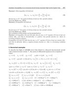
Examples: Repeated Eigenvalues
Example 1:
We have a 5 × 5 matrix A with eigenvalues . For , there is 1
distinct eigenvector a. For there is 1 distinct eigenvector b. From a, we generate the generalized
eigenvector c, and from c we can generate vector d. From the eigevector b, we generate the generalized
eigevector e. In order our eigenvectors are listed as:
[a c d b e]
Notice how c and d are listed in order after the eigenvector that they are generated from, a. Also, we
could reorder this as:
[b e a c d]
[Generalized Eigenvector Generating Equation]
Pa
g
e 89 of 209Control S

y
stems/Print version - Wikibooks, collection of o
p
en-content textbooks
10/30/2006htt
p
://en.wikibooks.or
g
/w/index.
p
h
p
?title=Control
_
S
y
stems/Print
_
version&
p
rintable=
y
es
because the generalized eigenvectors are listed in order after the regular eigenvector that they are
generated from. Regular eigenvectors can be listed in any order.
Example 2:
We have a 4 × 4 matrix A with eigenvalues . For we have two
eigevectors, a and b. For we have an eigenvector c.
We need to generate a fourth eigenvector, d. The only eigenvalue that needs another eigenvector is
, however there are already two eigevectors associated with that eigenvalue, and only one of them

will generate a non-trivial generalized eigenvector. To figure out which one works, we need to plug both
vectors into the generating equation:




If a generates the correct vector d, we will order our eigenvectors as:
[a d b c]
but if b generates the correct vector, we can order it as:
[a b d c]
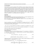
J
ordan Cannonical Form
I
f a matrix has a complete set of distinct eigenvectors, the
t
ransition matrix T can be defined as the matrix of those
e
igenvectors, and the resultan
t
transformed matrix will be a
d
iagonal matrix. However, if the eigenvectors are not unique, and
t
here are a number of generalized eigenvectors associated with the
m
atrix, the transition matrix T will consist of the ordered set of the regular eigenvectors and generalized
e
igenvectors. The regular eigenvectors tha
t
did not produce any generalized eigenvectors (if any) should be first in

t
he order, followed by the eigenvectors that did produce generalized eigenvectors, and the generalized
e
igenvectors that they produced (in appropriate sequence).
O
nce the T matrix has been produced, the matrix can be transformed by it and it's inverse:


T
he J matrix will be a
jordan block matrix
. The format of the jordan block matrix will be as follows:


For more information about
Jordan
Cannonical Form
, see:
Matrix Forms
Pa
g
e 90 of 209Control S
y
stems/Print version - Wikibooks, collection of o
p
en-content textbooks
10/30/2006htt
p
://en.wikibooks.or
g

/w/index.
p
h
p
?title=Control
_
S
y
stems/Print
_
version&
p
rintable=
y
es
Where D is the diagonal block produced by the regular eigenvectors that are not associated with generalized
eigenvectors (if any). The J
n
blocks are standard jordan blocks with a size corresponding to the number of
eigenvectors/generalized eigenvectors in each sequence. In each J
n
block, the eigenvalue associated with the
regular eigenvector of the sequence is on the main diagonal, and there are 1's in the super-diagonal.
System Response
Equivalence Transformations
If we have a non-singular n × n matrix P, we can define a transformed vector "x bar" as:


We can transform the entire state-space equation set as follows:

Where:
We call the matrix P the
equivalence transformation
between the two sets of equations.
It is important to note that the
eigenvalues
of the matrix A (which are of primary importance to the system) do not
change under the equivalence transformation. The eigenvectors of A, and the eigenvectors of are related by
the matrix P.
Pa
g
e 91 of 209Control S
y
stems/Print version - Wikibooks, collection of o
p
en-content textbooks
10/30/2006htt
p
://en.wikibooks.or
g
/w/index.
p
h
p
?title=Control
_
S

y
stems/Print
_
version&
p
rintable=
y
es
MIMO Systems
Multi-Input, Multi-Output
Systems with more then one input and/or more then one output are known as
Multi-Input Multi-Output

systems, or they are frequently known by the abbreviation
MIMO
. This is in contrast to systems that have only a
single input and a single output (SISO), like we have been discussing previously.
State-Space Representation
MIMO systems that are lumped and linear can be described easily with state-space equations. To represent
multiple inputs we expand the input u(t) into a vector
u
(t) with the desired number of inputs. Likewise, to
represent a system with multiple outputs, we expand y(t) into
y
(t), which is a vector of all the outputs. For this
method to work, the outputs must be linearly dependant on the input vector and the state vector.

Let's say that we have 2 outputs, y1 and y2, and 2 inputs, u1 and u2. These are related in our system through the
following system of differential equations:




now, we can assign our state variables as such, and produce our first-order differential equations:










And finally we can assemble our state space equations:


Pa
g
e 92 of 209Control S
y
stems/Print version - Wikibooks, collection of o
p
en-content textbooks
10/30/2006htt
p
://en.wikibooks.or

g
/w/index.
p
h
p
?title=Control
_
S
y
stems/Print
_
version&
p
rintable=
y
es


When we have multiple inputs or outputs, it is frequently common to use capital letters to denote vectors. For
instance, we can say that Y is the vector of all outputs, and U is the vector of all inputs.

Transfer Function Matrix
If the system is LTI and Lumped, we can take the Laplace Transform of the state-space equations, as follows:




Which gives us the result:

Where x(0) is the initial conditions of the system state vector. If the system is relaxed, we can ignore this term,
but for completeness we will continue the derivation with it.
We can separate out the variables in the state equation as follows:


Then factor out an
X
(s):


And then we can multiply both sides by the inverse of [sI-A] to give us our state equation:


N
ow, if we plug in this value for
X
(s) into our output equation, above, we get a more complicated equation:


And we can distribute the matrix
C
to give us our answer:


N
ow, if the system is relaxed, and therefore
x
(0) is 0, the first term of this equation becomes 0. In this case, we

can factor out a
U
(s) from the remaining two terms:
Pa
g
e 93 of 209Control S
y
stems/Print version - Wikibooks, collection of o
p
en-content textbooks
10/30/2006htt
p
://en.wikibooks.or
g
/w/index.
p
h
p
?title=Control
_
S
y
stems/Print
_
version&
p
rintable=
y
es