Operational Risk Modeling Analytics phần 2 ppsx
Bạn đang xem bản rút gọn của tài liệu. Xem và tải ngay bản đầy đủ của tài liệu tại đây (2.11 MB, 46 trang )
DISTRIBUTION FUNCTIONS AND RELATED CONCEPTS
29
fig.
2.7
Hazard
rate
function
for
Model
1
Fig.
2.8
Hazard
rate
function for
Model
2
calculations. In this book, such values will be arbitrarily defined
so
that the
function
is
right continu~us.~
0
A
variety of commonly
used
continuous distributions are presented in Chap-
ter
4,
and many discrete distributions are presented in Chapter
5.
An inter-
esting characteristic of
a
random variable
is
the value that is most likely to
occur.
'By arbitrarily defining the value of the density
or
hazard rate function at such
a
point,
it is clear that using either
of
them to obtain the survival function will work.
If
there is
discrete probability
at
this point (in which case these functions are left undefined). then
the density arid hazard functions are not sufficient to completely describe the probability
distribution.
30
BASIC PROBABILITY CONCEPTS
Definition 2.13
The
mode
of
a random variable
(or
equivalently
of
a distri-
bution) is the most likely value
of
th,e random variable.
For
a discrete variable
it is the value with the largest probability.
For
a continuous iiariable it is the
value
for
which the density function is largest.
Example
2.14
Determine the mode
for
Models
1-5.
Model
1:
The density function is constant. All values from
0
to
100
could
be the mode, or equivalently, it could be said that there is no (single) mode.
Model
2:
Model
3:
Model
4:
Model
4.
Model
5:
values from
0.
The density function is strictly decreasing and
so
the niode is
at
The probability is largest
at
0,
so
the mode is at
0.
As a mixed distribution, it
is
not possible to define a mode for
The density function is constant over two intervals, with higher
50
to
75.
The values between
50
and
75
are all modes, or equiv-
alently,
it
could be said that there is no single mode.
17
2.3
MOMENTS
The moments of a distribution are characteristics that can be used in describ-
ing a distribution.
Definition 2.15
The
Icth
raw
moment
of
a distribution is the expected (av-
erage) value
of
the Icth power
of
the random variable, provided
it
exists. It is
denoted
by
E(Xk)
or
by
pk.
The first raw moment is called the
mean
and is
usually denoted
by
p.
For
random variables that take on only nonnegative values (i.e., Pr(X
2
0)
=
l),
k
may be any real number. When presenting formulas for calculating
this quantity, a distinction between continuous and discrete variables must be
made. The formula for the kth raw moment is
zkf(x)dz
if
the random variable is
of
the continuous type
=
x:p(x,)
if
the random variable is of the discrete type,
3
(2.1)
where the sum is
to
be taken over all possible values of
z~j.
For
mixed mod-
els, evaluate the formula by integrating with respect to its density function
wherever the random variable is continuous and by summing with respect
to
its
probability function wherever the random variable is discrete and adding
the results. Finally, it should be noted that it is possible that the integral
or
MOMENTS
31
sum will not converge to
a
finite value, in which case the moment is said not
to exist.
Example
2.16
Determine the first two raw moments
for
each
of
the five
models.
The subscripts on the random variable
X
indicate which model is being
used.
100
E(X1)
=
1
x(O.Ol)dx
=
50,
E(Xf)
=
1
x2(0.01)dx
=
3,333.33,
100
dx
=
1,000,
(.
+
2,000)4
dx
=
4,000,000,
O0
3(2,000)3
(x
+
2,000)4
E(X;)
-1
x2
E(X3)
=
O(0.5)
+
l(0.25)
+
2(0.12)
+
3(0.08)
+
4(0.05)
=
0.93,
E(X:)
=
O(0.5)
+
l(0.25)
+
4(0.12)
+
g(0.08)
+
16(0.05)
=
2.25,
E(X4)
=
O(0.7)
+
x(0.000003)e-0~00001”dx
=
30,000,
Lm
E(X2)
=
02(0.7)
+
x2(0.000003)e-0~000012d~
=
6,000,000,000,
im
1-50
1-75
E(X5)
=
z(O.Ol)dx
+
z(0.02)dz
=
43.75,
Before proceeding further, an additional model will be introduced. This
one looks similar to Model
3,
but with one key difference. It is discrete,
but with the added requirement that all
of
the probabilities must be integral
multiples of some number. In addition, the model must be related to sample
data in a particular way.
Definition
2.17
The
empirical
model
is a discrete distribution based
on
a
sample
of
size
n
that assigns probability
l/n
to each data point.
Model
6
Consider a sample of size
8
in which the observed data points
were
3, 5,
6,
6, 6,
7, 7,
and
10.
The empirical model then has probability
function
32
BASIC PROBABILITY CONCEPTS
0.125,
x
=
3,
0.125,
x
=
5,
0.25,
x
=
7,
0.125,
x
=
10.
I?
Alert readers will note that many discrete models with finite support look
like empirical models. Model
3
could have been the empirical model €or a
sample of size 100 that contained 50 zeros, 25 ones,
12
twos,
8
threes, and 5
fours. Regardless, we will use the term empirical model only when it is based
on an actual sample. The two moments for Model
6
are
E(X6)
=
6.25,
E(Xi)
=
42.5
using the same approach as in Model
3.
It
should
be
noted that the mean
of this random variable is equal to the sample arithmetic average (also called
the sample mean).
Definition
2.18
The
kth
central moment
of
a random variable
is
the ex-
pected value
of
the kth power
of
the deviation
of
the variable from its mean.
It
is
denoted
by
E[(X
-
P)~]
or
by
pk.
The second central moment
is
usually
called the
variance
and often denoted
g2,
and its square root,
u,
is culled
the
standard deviation.
The ratio
of
the standard deviation to the mean is
called the
coefficient
of
variation.
The ratio
of
the third central moment
to the cube
of
the standard deviation,
y1
=
p3/a3,
is called the
skewness.
The ratio
of
the fourth central moment
to
the fourth power
of
the standard
deviation,
72
=
p4/a4,
is called the
Ic~rtosis.~
For distributions of continuous and discrete types, formulas for calculating
central moments are
pk
=
-
PIk]
00
(x
-
~)~f(z)dx
if
the random variable
is
continuous
=
c(xj
-
p)‘p(xj)
if
the random variable is discrete.
(2.2)
j
In reality, the integral need be taken only over those
x
values where
f(z)
is
positive because regions where
f(x)
=
0 do not contribute to the value of the
integral. The standard deviation is a measure
of
how much the probability
‘It
would be more accurate to call these items the “coefficient
of
skewness” and “coefficient
of
kurtosis” because there are other quantities that
also
measure asymmetry
and
flatness.
The simpler expressions
will
be
used
in this text.
MOMENTS
33
is spread out over the random variable’s possible values. It is measured in
the same units
a.s
the random variable itself. The coefficient of variation
measures the spread relative to the mean. The skewness is a measure of
asymmetry.
A
symmetric distribution has a skewness of zero, while a positive
skewness indicates that probabilities to the right tend to be assigned to values
further from the mean than those to the left. The kurtosis measures flatness
of the distribution relative to
a
normal distribution (which has
a
kurtosis of
3).
Kurtosis values above
3
indicate that (keeping the standard deviation
constant), relative to a normal distribution, more probability tends to be at
points away from the mean than at points near the mean. The coefficients of
variation, skewness, and kurtosis are all dimensionless quantities.
There is
a
link between raw and central moments. The following equation
indicates the connection between second moments. The development uses the
continuous version from equations
(2.1)
and
(2.2),
but the result applies to
all random variables.
00
m
(x
-
p)2f(x)dx
=
(2
-
2xp
+
p2)
f
(z)dx
IL2
=
I,
L
=
E(X2)
-
2pE(X)
+
p2
=
pk
-
p2.
(2.3)
Example
2.19
The density function
of
the gamma distribution with
appears to be positively skewed (see Figure
2.9).
Demonstrate that this is true
and illustrate with graphs.
The first three raw moments of the gamma distribution can be calculated
as
cr6,
(Y((Y
+
1)Q2,
and
CY((Y
+
1)(a
+
2)e3.
From formula
(2.3)
the variance is
o02,
and from the solution to Exercise
2.5
the third central moment is
2ae3.
Therefore, the skewness is
2cr-’I2.
Because
(Y
must be positive, the skewness
is always positive. Also, as
(Y
decreases, the skewness increases.
Consider the following two gamma distributions. One has parameters
(Y
=
0.5
and
6
=
100,
while the other has
a
=
5
and
6
=
10.
These have the same
mean, but their skewness coefficients are 2.83 and 0.89, respectively. Figure
2.9
demonstrates the difference.
I?
Note that when calculating the standard deviation for Model
6
in Exercise
2.6
the result
is
the sample standard deviation using
n
as opposed to the more
commonly used
n
-
1
in the denominator. Finally, it should be noted that
when calculating moments it is possible that the integral or sum will not exist
(as is the case for the third and fourth moments for Model
2).
For the models
we typically encounter, the integrand and summand are nonnegative and
so
failure to exist implies that the required limit that gives the integral or
sum
is infinity. See Example
4.14
for an illustration.
34
BASIC PROBABILITY CONCEPTS
0.09
,
1
Fig.
2.9
Densities
of
f(z)
-gamma(0.5,100)
and
g(z)
~gamma(5,lO)
Definition
2.20
For a given value
of
a
threshold
d
with Pr(X
>
d)
>
0,
the
excess
loss
variable
is
Y
=
X
-
d
given that X
>
d.
Its expected value,
ex(d)
=
e(d)
=
E(Y)
=
E(X
-
d/X
>
d),
is called the
mean excess
loss
function.
Other names for this expectation,
which are used
an
other contexts, are
mean residual life function
and
expectation
of
life.
The conditional random variable
X
-
dlX
>
d
is
a
left-truncated and
shifted random variable.
It is left-truncated because values below
d
are not
considered; i.e., they are ignored. It is shifted because
d
is subtracted from
the remaining values.
When
X
is a payment variable, as in the insurance
context, the mean excess
loss
is the expected amount paid given that there
is
a
positive payment in excess of
a
deductible of
d.
In the demographic context,
X
is interpreted as the age
at
death; and, the mean excess
loss
(expectation
of life) is the expected remaining lifetime given that the person is alive at age
d.
The lcth moment of the excess loss variable is determined from
if the variable is of the continuous type
S,"(x
-
d)"(z)dz
e%(d)
=
1
-
F(d)
if the variable is of the discrete type.
(2.4)
-
CZ,>d(X3
-
d)"(xJ
-
1
-
F(d)
Here,
e$(d)
is
defined only if the integral or sum converges. There is a partic-
ularly convenient formula for calculating the first moment. The development
is given below for the continuous version, but the result holds for all ran-
dom variables. The second line is based on an integration by parts where the
MOMENTS
35
Definition
2.21
The
left-censored and shifted random variable
is
The random variable is left-censored because values below
d
are not ignored
but are, in effect, set equal to
0.
There is no standard name
or
symbol for
the moments of this variable. For events such
as
losses that are measured in
a monetary unit, the distinction between the excess loss variable and the left-
censored and shifted variable is important. In the excess loss situation, any
losses below the threshold
d
are not recorded in any way. In the operational
risk context, if small losses below some threshold
d
are not recorded
at
all,
the distribution is left-truncated. If the number of such small (and treated
as
zero) losses is recorded, the loss amount random variable is left-censored.
The moments can be calculated from
roo
E[(X
-
d)'",]
=
1
(z
-
d)'f(z)dz
if the variable is of the continuous type,
d
=
(zj
-
d)'p(zj)
if
the variable is of the discrete type.
x3
>d
(2.6)
Example
2.22
Construct graphs to illustrate the diference between the ex-
cess
loss
random variable and the left-censored and shifted random variable.
The two graphs in Figures
2.10
and
2.11
plot the modified variable
Y
as
a
function of the unmodified variable
X.
The only difference is that for
X
values below
100
the variable is undefined while for the left-censored and
0
shifted variable it is set equal to zero.
The next definition provides a complementary function to the excess loss.
Definition
2.23
The
limited loss random variable
is
x,
x
<
u,
u,
x
2
u.
Y=xAu=
36
BASIC PROBABILITY CONCEPTS
200
150
2.
100
50
0
-50
1
I
0
50
100
1
50
200 250
300
X
Fig.
2.10
Excess
loss
variable
-50
I
I
0
50
100
150
200
250
300
X
f;g.
2.11
Left
censored and shifted variable
Its
expected
value,
E[X
A
u],
is
culled
the
limited expected value.
This variable could also be called the
right-censored random variable.
It is right-censored because values above
u
are set equal to
u.
In the opera-
tional risk context a limit to a
loss
can occur
if
losses in excess of that amount
are insured
so
that the excess of a loss over the limit
u
is covered by an insur-
ance contract. The company experiencing the operational risk loss can lose
at
most
u.
Note that
(X
-
d)+
+
(X
A
d)
=
X.
An insurance analogy is useful here.
Buying one insurance contract with a limit of
d
and another with a deductible
of
d
is equivalent
to
buying full coverage. This is illustrated in Figure
2.12.
Buying only the insurance contract with a deductible
d
is equivalent to self-
insuring losses up to
d.
MOMENTS
37
250
200
50
0
0
20
40
60 80
100
120
140
160 180 200
LOSS
Fig.
2.12
Limit
of
100
plus deductible
of 100
equals full coverage
Simple formulas for the kth moment of the limited loss variable are
E[(X
A
u)~]
=
/:
z'f(z)dz
+
uk[l
-
F(u)]
if the random variable is continuous
=
c
z;p(zj)
+
uk[l
-
F(u)]
53
5
if the random variable is discrete.
Another interesting formula is derived as follows:
0
=
z"(z)O_,
-
Lm
kz"'F(x)dz
-
z"(2);
+
1%
kz"-'-
F(z)dz
+
UkF(U)
-
-
-
s,
kz"-1F(z)dz
+
I"
kzk-'F(z)dz,
0
(2.8)
where the second line uses integration by parts. For
k
=
1,
we have
0
E(X
A
u)
=
-
F(z)dz
+
1
F(z)ds.
L
If the
loss
distribution has only nonnegative support, then the first term in
the right-hand side of the above two expressions vanishes. The kth limited
moment of many common continuous distributions is presented in Chapter
38
BASIC PROBABILITY CONCEPTS
4.
Exercise 2.12 asks you to develop
a
relationship between the three first
moments introduced previously.
2.4
QUANTILES
OF
A DISTRIBUTION
One other value of interest that may be derived from the distribution function
is the quantile function.
It
is the value of the random variable corresponding
to a particular value of the distribution function. It can be thought of
as
the
inverse of the distribution function.
A
percentile
is
a quantile that is expressed
in percentage terms.
Definition
2.24
The lOOpth
percentile
(or
quantile)
of
a random variable
X is any value
xp
such that
F(xp-)
5
p
5
F(xp).
The 50th percentile,
20.5
is called the
median.
If the distribution function has a value of
p
for exactly one
2
value, then
the percentile is uniquely defined. In addition, if the distribution function
jumps from a value below
p
to a value above
p,
then the percentile is
at
the
location of the jump. The only time the percentile is not uniquely defined
is when the distribution function
is
constant at a value of
p
over
a
range of
values. In that case, any value in that range can be used as the percentile.
Example
2.25
Determine the 50th and 80th percentiles for Models
1
and
3.
For Model
1,
the pth percentile can be obtained from
p
=
F(zp)
=
0.01~~
and
so
xp
=
loop,
and in particular, the requested percentiles are
50
and
80
(see Figure
2.13).
For Model
3
the distribution function equals
0.5
for all
0
5
z
<
1
and
so
all such values can be the 50th percentile. For the 80th
percentile, note that at
2
=
2
the distribution function jumps from
0.75
to
0
0.87
and
so
50.8
=
2
(see Figure 2.14).
2.5
GENERATING FUNCTIONS
Sums of random variables are important in operational risk. Consider the op-
erational risk losses arising from
k
units in the company. The total operational
risk losses over all
k
units is the
sum
of the losses for the individual units.
Thus it is useful to be able to determine properties of
Sk
=
XI
+
. . .
+
Xk.
The first result is a version of the central limit theorem.
Theorem
2.26
For
a random variable
Sk
as defined above,
E(Sk)
=
E(X1)+
.
.
.
+E(Xk).
Also,
ifX1,.
.
,
,
xk
are mutually independent,
Var(Sk)
=Var(X1)+
. .
.
+Var(Xk).
If
the random variables XI,
Xz,
. . . ,
Xk
are mutually indepen-
GENERATING FUNCTIONS
39
1
0.9
0.8
0.7
0.6
&
0.5
0.4
0.3
0.2
0.1
0
4
1.2
1
0.8
&.
0.6
4
0.4
0.2
0
T
~
-
F(x)
'
- -
50th percentile
I-
-
-
.80th percentile
I
0
10
20
30
40
50
60
70
80
90
100
X
Fig.
2.13
Percentiles
for
Model
1
0
1
2
3
4
5
X
fig.
2.14
Percentiles
for
Model
3
dent and their first two moments meet certain regularity conditions, the stan-
dardized sum
[Sk
-E(Sk)]/dw has
a
limiting normal distribution with
mean
0
and variance
1
as
k
becomes infinitely large.
Obtaining the exact distribution of
Sk
may be very difficult.
We
can rely
on
the central limit theorem to give
us
a normal approximation for large values
of
k.
The
quality of the approximation depends in the size of
k
and on the
shape of the distributions
of
the random variables
XI,
Xz,
.
. .
,
Xk.
Definition
2.27
For a random variable
X,
the
moment generating func-
tion
(mgf) is
hfx(t)
=
E(etx) for all
t
for which the expected value exists.
The
probability generating function
(pgf) is
Px(.z)
=
E(zx)
for
all
z
for
which the expectation exists.
40
BASIC PROBABILITY CONCEPTS
Note that
Mx(t)
=
Px(et) and
P,y(z)
=
Mx(1nz). Often the mgf is used
for continuous random variables and the pgf for discrete random variables. For
us,
the value of these functions is not
so
much that they generate moments or
probabilities but that there is
a
one-to-one correspondence between a random
variable's distribution function and its mgf and pgf (i.e., two random variables
with different distribution functions cannot have the same mgf or
pgf).
The
following result aids in working with sums of random variables.
Theorem
2.28
Let
sk
=
XI
+
.
.
.
+
xk,
where the random variables
in
the
sum are mutually independent. Then the exact distribution
of
the sum is given
by
the
mgf
and
pgf
as Ms,(t)
=
n:=,
Mx,(t) and
Psk(z)
=
rr,"=,
Px,(z)
provided
all
the component mgfs and pgf. exist.
Proof:
We use the fact that the expected product of independent random
variables is the product of the individual expectations. Then,
k
k
=
E(etxJ)
=
n
Mx,
(t).
3=1
j=1
A
similar argument can be used for the pgf.
0
Example
2.29
Show that the sum
of
independent gamma random variables,
each with the same value
of
8,
has a gamma distribution.
The moment generating function
of
a gamma variable is
Now let
Xj
have
a
gamma distribution with parameters
aj
and
8.
Then the
moment generating function of the sum is
which is the moment generating function of
a
gamma distribution with
para-
meters
a1
+.
.
.
+
ak
and
6.
0
EXERCISES
41
Example
2.30
Obtain the
mgf
and
pgf
for
the
Poisson
distribution with
pf
The pgf is
Then the mgf is
Mx(t)
=
Px(et)
=
exp[X(et
-
I)].
0
2.6
EXERCISES
2.1
Determine the distribution, density, and hazard rate functions for Model
5.
2.2
Construct graphs of the distribution function for Models
3-5.
Also
graph
the density
or
probability function
as
appropriate and the hazard rate func-
tion, where
it
exists.
2.3
A
random variable
X
has density function
f(~)
=
4~(1
+
x’)-~,
x
>
0.
Determine the mode of
X.
2.4
A
nonnegative random variable has
a
hazard rate function of
h(x)
=
A
+
e2x,
x
2
0.
You are also given
F(0.4)
=
0.5.
Determine the value of
A.
2.5
Develop formulas similar to
(2.3)
for
p3
and
p4.
2.6
Calculate the standard deviation, skewness, and kurtosis for each of the
six models.
2.7
A
random variable has a mean and
a
coefficient of variation of
2.
The
third raw moment is
136.
Determine the skewness.
2.8
Determine the skewness of a gamma distribution that has
a
coefficient of
variation of
1.
2.9
Determine the mean excess
loss
function for Models
1-4.
Compare the
functions for Models
1,
2,
and
4.
2.10
For two random variables,
X
and
Y,
ey(30)
=
ex(30)
+
4.
Let
X
have
a uniform distribution on the interval from
0
to
100
and let
Y
have a uniform
distribution on the interval from
0
to
w.
Determine
w.
42
BASIC PROBABILITY CONCEPTS
2.11
A
random variable has density function
f(x)
=
A-'e-"/',
x,A
>
0.
Determine
.(A),
the mean excess loss function evaluated
at
z
=
A.
2.12
Show that the following relationships holds:
E(X)
=
E(X
A
d)
+
F(d)e(d)
(2.9)
=
E(X
Ad)
+
E
[(X
-
d)+]
.
2.13
Determine the limited expected value function for Models 1-4. Do this
using both (2.7) and (2.9). For Models
1
and 2 also obtain the function using
(2.8).
2.14
Define
a
right-truncated variable and provide a formula for its kth mo-
ment.
2.15
The distribution of individual losses has pdf
f(z)
=
2.5~-~'~,
z
>_
1.
Determine the coefficient of variation.
2.16
Possible
loss
sizes are for $100, $200,
$300,
$400, or $500. The prob-
abilities for these values are 0.05,
0.20,
0.50, 0.20, and 0.05, respectively.
Determine the skewness and kurtosis for this distribution.
2.17
Losses follow
a
Pareto distribution with
(Y
>
1
and
0
unspecified. Deter-
mine the ratio
of
the mean excess
loss
function
at
x
=
20
to the mean excess
loss function at
x
=
0.
2.18
The cdf of
a
random variable is
F(s)
=
1
-
x-~,
z
2
1.
Determine the
mean, median, and mode of this random variable.
2.19
Determine the 50th and 80th percentiles for Models
2,
4,
5,
and
6.
2.20
Losses have a Pareto distribution with parameters
(Y
and
0.
The 10th
percentile is
0
-
k.
The 90th percentile is 58
-
3k.
Determine the value
of
a.
2.21
Losses have a Weibull distribution with cdf
F(x)
=
1
-
e-(Z'Qy
z
>
0.
The 25th percentile is
1,000
and the 75th percentile is
100,000.
Determine
the value of
T.
2.22
Consider 16 independent risks, each with
a
gamma distribution with
parameters
(Y
=
1
and
6
=
250. Give an expression using the incomplete
gamma function for the probability that the sum of the losses exceeds
6,000.
Then approximate this probability using the central limit theorem.
EXERCISES
43
2.23
The sizes
of
individual operational risk losses have the Pareto distribu-
tion with parameters
a
=
8/3,
and
19
=
8,000.
Use the central limit theorem
to approximate the probability that the sum
of
100
independent losses will
exceed 600,000.
2.24
The sizes
of
individual operational risk losses have the gamma distrib-
ution with parameters
LY
=
5
and
8
=
1,000.
Use the central limit theorem to
approximate the probability that the sum
of 100
independent losses exceeds
525,000.
2.25
A
sample
of
1,000
operational risk losses produced
an
average loss
of
$1,300
and
a
standard deviation
of
$400.
It is expected that
2,500
such losses
will occur next year. Use the central limit theorem to estimate the probability
that total losses will exceed the expected amount
by
more than
1%.
This Page Intentionally Left Blank
3
Measures
of
risk
It
is impossible to make everything foolproof, because fools are
so
ingenious.
-Murphy
3.1
INTRODUCTION
Probability-based models provide a description of risk exposure. The level of
exposure to risk is often described by one number,
or
at least a small set of
numbers. These numbers are necessarily functions
of
the model and are often
called “key risk indicators.” Such key risk indicators indicate to risk managers
the degree to which the company is subject to particular aspects of risk. In
particular, Value-at-Risk (VaR) is a quantile of the distribution
of
aggregate
risks.
Risk
managers often look at “the chance of an adverse outcome.” This
can be expressed through the VaR
at
a particular probability level. VaR
can also be used in the determination of the amount of capital required to
withstand such adverse outcomes. Investors, regulators, and rating agencies
are particularly interested to the company’s ability to withstand such events.
VaR suffers from some undesirable properties.
A
more informative and
more useful measure of risk is Tail-Value-at-Risk (TVaR). It has arisen inde-
pendently in a variety
of
areas and has been given different names including
Conditional-Value-at-Risk (CVaR), Conditional Tail Expectation (CTE) and
Expected Shortfall
(ES).
In this book we first focus on developing the under-
lying probability model, and then apply
a
measure
of
risk to the probability
45
46
MEASURES
OF
RISK
model to provide the risk manager with useful information in
a
very simple
format.
The subject of the determination of risk capital has been of active inter-
est to researchers, of interest to regulators of financial institutions, and of
direct interest to commercial vendors of financial products and services. At
the international level, the actuarial and accounting professions and insurance
regulators through the International Accounting Standards Board, the Inter-
national Actuarial Association, and the International Association of Insurance
Supervisors are all active in developing
a
framework for accounting and capital
requirements for insurance companies.
Similarly, the Basel Committee and
the Bank of International Settlements have been developing capital standards
for use by banks.
3.2
RISK
MEASURES
Value-at-Risk (Van) has become the standard risk measure used to evaluate
exposure to risk. In general terms, the VaR is the amount of capital required
to ensure, with
a
high degree of certainty, that the enterprise doesn’t become
technically insolvent. The degree of certainty chosen is arbitrary. In prac-
tice, it can be
a
high number such as 99.95% for the entire enterprise, or it
can be much lower, such as 95%, for
a
single unit or risk class within the
enterprise. This lower percentage may reflect the inter-unit or inter-risk type
diversification that exists.
The promotion of concepts such
as
VaR has prompted the study of risk
measures by numerous authors (e.g., Wang [122], [123]). Specific desirable
properties of risk measures were proposed as axioms in connection with risk
pricing by Wang, Young, and Panjer [la51 and more generally in risk mea-
surement
by
Artzner et al.
[6].
We consider
a
random variable
Xj
representing the possible losses (in our
case losses associated arising from operational risk) for a business unit or
particular class of risk. Then the total or aggregate losses for
n
units or risk
types is simply the sum of the losses for all units
x
=
XI
fX2
+
.
+x,,.
The study of risk measures has been focused on ensuring consistency be-
tween the way risk is measured
at
the level of individual units and the way
risk is measured after the units are combined. The concept of “coherence” of
risk measures was introduced by Artzner et
a1
IS].
This paper is considered
to be the groundbreaking paper in the area of risk measurement.
The probability distribution
of
the total operational losses
X
depends not
only on the distributions
of
the operational losses for the individual business
units but also on the interrelationships between them. Correlation
is
one such
measure of interrelationship. The usual definition of correlation (as defined in
RISK
MEASURES
47
statistics) is a simple linear relationship between two random variables. This
linear relationship may not be adequate to capture other (nonlinear) aspects
of the relationship between the variables. Linear correlation does perform
perfectly for describing interrelationships in the case where the operational
losses from the individual business units form
a
multivariate normal distribu-
tion. Although the normal assumption is used extensively in connection with
the modeling of changes in the logarithm of prices in the stock markets, it
may not be entirely appropriate for modeling many processes including op-
erational loss processes. For financial models and applications, where much
of
the theory is based on Brownian motion or related processes resulting in
normal distributions, the normal distribution model serves
as
a
benchmark
and provides insight into key relationships. From the insurance field, it is well
known that skewed distributions provide better descriptions of losses than
symmetric distributions.
There are two broad approaches to the application of risk measurement to
the determination of capital needs
for
complex organizations such
as
insurance
companies and banks. One approach is to develop
a
mathematical model for
each of the risk exposures separately and assign
a
capital requirement to each
exposure based on the study of that risk exposure. This is often called the
risk-based capital (RBC) approach in insurance and the Base1 approach in
banking. The total capital requirement is the (possibly adjusted) sum of
the capital requirements for each risk exposure. Some offset may be possible
because of the recognition that there may be
a
diversification or hedging
effect of risks that are not perfectly correlated. The second approach uses
an integrated model of the entire organization (the internal model approach).
In this approach,
a
mathematical model is developed to describe the entire
organization. The model incorporates all interactions between business units
and risk types in the company. All interrelationships between variables are
built into the model directly. Hence, correlations are captured in the model
structure. In this approach, the total capital requirement for all types of
risks can be calculated
at
the highest level in the organization. When this
is the case, an allocation
of
the total capital back to the units is necessary
for
a
variety of business management or solvency management reasons. The
first approach to capital determination is often referred to
as
a
“bottom-up”
approach, while the second is referred to
as
a
L‘top-do~n’’ approach.
A
risk measure is
a
mapping from the random variable representing the
loss associated with the risks to the real line (the set of all real numbers).
A
risk measure gives a single number that is intended to quantify the risk
exposure. For example, the standard deviation, or
a
multiple of the standard
deviation of a distribution, is
a
measure of risk because it provides a measure
of uncertainty. It is clearly appropriate when using the normal distribution.
One of the other most commonly used risk measures in the fields of finance and
statistics is the quantile of the distribution or the Value-at-Risk (VaR). VaR
is
the size of loss for which there is
a
small (e.g.
1%)
probability of exceedence.
VaR is the most commonly used method for describing risk because it
is
48
MEASURES
OF
RISK
easily communicated. For example an event
at
the
1%
per year level is often
described as the “one in a hundred year” event. However, for some time
it
has
been recognized that Van suffers from major problems. This will be discussed
further after the introduction of coherent risk measures.
Throughout this book, the risk measures are denoted by the function
p(X).
It is convenient to think of p(X)
as
the amount of assets required for the risk
X. We consider the set
of
all random variables
X,
Y
such that both cX and
X
+
Y
are also in the set. This is not very restrictive, but it does eliminate
risks that are measured as percentages as with Model
1
of the Chapter
2.
Nonnegative loss random variables that are expressed in dollar terms and
that have no upper limit satisfy the above requirements.
Definition
3.1
A
coherent
risk
measure
p(X)
is defined as one that has
the following four properties for any two bounded
loss
random variables X and
Y:
1.
Subadditivity:
p(X
+
Y)
5
p(X)
+
p(Y).
2.
Monotonicity:
If
X
5
Y
for
all
possible outcomes, then
p(X)
5
p(Y).
3.
Positive homogeneity: For any positive constant c, p(cX)
=
cp(X).
4.
Translation invariance:
For
any positive constant c,
p(X+c)
=
p(X)+c.
Subadditivity means that the risk measure (and hence the capital required
to support
it)
for two risks combined will not be greater than for the risks
treated separately. This reflects the fact that there should be some diversifi-
cation benefit from combining risks. This is necessary
at
the corporate level,
because otherwise companies would find it to be an advantage to disaggregate
into smaller companies. There has been some debate about the appropriate-
ness of the subadditivity requirement. In particular, the merger of several
small companies into
a
larger one exposes each of the small companies to the
reputational risk of the others. We will continue to require subadditivity as
it
reflects the possibility of diversification.
Monotonicity means that if one risk always has greater losses than another
risk under all circumstances, the risk measure (and hence the capital required
to support it) should always be greater. This requirement should be self-
evident from an economic viewpoint.
Translation invariance means that there is no additional risk (and hence
capital required to support it) for an additional risk for which there is no
additional uncertainty. In particular, by making
X
identically zero, the assets
required
for
a
certain outcome is exactly the value
of
that outcome. Also,
when a company meets the capital requirement by setting up additional risk-
free capital, the act of injecting the additional capital does not, in itself, trigger
a further injection
(or
reduction) of capital.
Positive homogeneity means that the risk measure (and hence the capital
required to support it) is independent of the currency in which the risk is
measured. Equivalently, it means that, for example, doubling the exposure to
a particular risk requires double the capital. This is sensible because doubling
the position provides no diversification.
RISK
MEASURES
49
Risk measures satisfying these four criteria are deemed to be coherent.
There are many such risk measures.
Example
3.2
(Standard deviation principle)
The standard deviation is a
measure
of
uncertainty
of
a distribution. Consider a
loss
distribution with
mean
p
and standard deviation
a.
The quantity
p
+
ka,
where
k
is the same
fixed constant for all distributions, is a risk measure (often called the
stan-
dard deviation principle).
The coeficient k is usually chosen to ensure
that losses will exceed the risk measure for some distribution, such as the nor-
mal distribution, with some specified
small
probability. The standard deviation
principle is not a coherent risk measure. Why? While properties
1,
3,
and
4
0
hold, property
2
does not. Can you construct a counterexample?
If
X
follows the normal distribution,
a
value of
k
=
1.645 results in an
exceedence probability of Pr
(X
>
p
+
ka)
=
5%.
Similarly, if
k
=
2.576,
then Pr
(X
>
p
+
ka)
=
0.5%.
However, if the distribution is not normal,
the same multiples of the standard deviation will lead to different exceedence
probabilities. One can also begin with the exceedence probability, obtaining
the quantile
/I
+
ka
and the equivalent value of
k.
This is the key idea behind
Value-at-Risk.
Definition
3.3
Let
X
denote a
loss
random variable. The
Value-at-Risk
of
X
at the
loop%
level, denoted
VaR,(X)
or
+,
is the
1OOp
percentile (or
quantile)
of
the distribution
of
X.
For
continuous distributions, we can simply write VaRp(X)
for
random
variable
X
as the value
of
zp
satisfying
Pr (X
>
xP)
=
p.
It
is well known that VaR does not satisfy one of the four criteria for coherence,
the subadditivity requirement. The failure of
VaR
to be subadditive can
been shown by
a
simple counter but extreme example inspired by a more
complicated one from Wirch [128].
Example
3.4
(Incoherence of Van)
Let
Z
denote a
loss
random variable
of
the continuous type with cdf at
$1,
$90,
and
$100
satisfying the following three
equations:
Fz(1)
=
0.91,
Fz(90)
=
0.95,
Fz(100)
=
0.96.
The
95%
quantile, the VaRS,%(Z) is
$90
because there is a
5%
chance
of
exceeding
$90.
50
MEASURES
OF
RISK
Suppose that we now split the risk
Z
into two separate (but dependent)
risks
X
and
Y
such that the two separate risks
in
total are equivalent to risk
2,
that is,
X
+
Y
=
Z.
One way
to
do this is by defining risk
X
as the
loss
if
it
falls up to
$100,
and zero otherwise. Similarly define risk
Y
as the
loss
if
it
falls over
$1
00,
zero otherwise. The cdf for risk
X
satisfies
Fx
(1)
=
0.95,
Fx(90)
=
0.99,
Fx(100)
=
1.
indicating a 95% quantile
of
$1.
Similarly the cdf
for
risk
Y
satisfies
Fz(0)
=
0.96
indicating that there
is a 96% chance
of
no
loss.
Therefore the 95% quantile cannot exceed
$0.
Consequently, the sum
of
the 95% quantiles for
X
and
Y
is less than the
VaRgS%(Z) which violates subadditivity.
0
Although this example may appear to be somewhat artificial, the existence
of such possibilities creates opportunities for strange
or
unproductive manip-
ulation. Therefore we focus on risk measures that are coherent.
3.3
TAI
L-VA
LU
E-
AT-
RISK
As
a
risk measure, Value-&Risk is used extensively in financial risk manage-
ment of trading risk over
a
fixed (usually relatively short) time period. In
these situations, the normal distribution are often used
for
describing gains
or
losses.
If
distributions of gains
or
losses are restricted to the normal distri-
bution, Value-at-Risk satisfies all coherency requirements. This is true more
generally for elliptical distributions, for which the normal distribution is
a
special case. However, the normal distribution is generally not used
for
de-
scribing operational risk losses
as
most loss distributions have considerable
skewness. Consequently, the use of Van is problematic because of the lack
of
subadditivity.
Definition
3.5
Let
X
denote a
loss
random variable. The Tail- Value-at-Risk
of
X
at the loop% confidence level, denoted TVaR,(X), is the expected
loss
given that the
loss
exceeds the
loop
percentile (or quantile)
of
the distribution
of
X.
For
the sake
of
notational convenience, we shall restrict consideration to
continuous distributions. This avoids ambiguity about the definition of Van.
In general, we can extend the results to discrete distributions
or
distributions
of mixed type by appropriately modifying definitions.
For
practical purposes,
it is generally sufficient to think in terms of continuous distributions.
TAIL- VAL UE-AT-
RISK
51
We can simply write TVaR,(X)
TVaR,(X)
=
E
(X
for random variable
X
as
where
F(z)
is the cdf of
X.
Furthermore, for continuous distributions, if the
above quantity is finite, we can use integration by parts and substitution to
rewrite this
as
-
s,’
vartzL(X)
du
-
1-P
Thus, TVaR can be seen to average all VaR values above confidence level
p.
This means that TVaR tells
us
much more about the tail of the distribution
than Van alone.
Finally, TVaR can also be written
as
TVaRp(X)
=
E(X
I
X
>
xP)
=
xp
+
=
VaRp(x)
+
e(zp)
Jx;
t.
-
ZP)
dF(x)
1
-
F(Xp)
where e(xp) is the mean excess loss function. Thus TVaR is larger than
the corresponding VaR by the average excess of all losses that exceed Van.
TVaR has also been developed independently in the insurance field and called
Conditional Tail Expectation
(CTE) by Wirch
[128]
and widely known
by that term in North America. It has also been called
Tail Conditional
Expectation
(TCE). In Europe,
it
has
also
been called
Expected Shortfall
(ES).
(See Tasche
[113]
and Acerbi and Tasche
[3]).
Overbeck
1871
also discusses VaR and TVaR as risk measures. He argues
that VaR
is
an “all or nothing” risk measure, in that if an extreme event
in excess of the Van threshold occurs, there is no capital to cushion losses.
He also argues that the VaR quantile in TVaR provides
a
definition of “bad
times,” which are those where losses exceed the VaR threshold, thereby not
using
up
all available capital when TVaR is used to determine capital. Then
TVaR provides the average excess loss in “bad times,” that is, when the VaR
“bad times” threshold has been exceeded.
Example
3.6
(Normal distribution)
mean
p,
standard deviation
0,
and
Consider a normal distribution with
52
MEASURES
OF
RISK
Let
$(x)
and
@(x)
denote the pdf and the cdf
of
the standard normal dis-
tribution
(p
=
0,
u
=
1). Then
VaR,(X)
=
p
+
a@-'
(p)
and, with
a
bit
of
calculus,
it
can be shown that
Note that,
in
both cases, the
risk
measure can be translated to the standard
0
deviation principle with an appropriate choice
of
k.
Example
3.7
(t
distribution)
Consider a
t
distribution with location para-
meter
p,
scale parameter
u,
with
u
degrees
of
freedom and pdf
Let
t(x)
and
T(x)
denote the pdf and the cdf
of
the standardized t distrib-
ution
(p
=
0,
LT
=
1) with
v
>
2
degrees
of
freedom. Then
VaR,(X)
=
p
+
uT-'
(p)
and, with some more calculus, it can be shown that
Example
3.8
(Exponential distribution)
Consider an exponential distribu-
tion with mean
6
and
1
0
f(x)
=
-
exp
(-;)
,
2
>
0.
Then
VaR,(X)
=
Oln(1
-p)
and
TV~R,(X)
=
va~,(x)
+
e.
The excess of TVaR over
Van
is
a
constant
8
for
all
values ofp because
of
the memoryless property
of
the exponential distribution.
TAIL- VA L UE-A
T-
RISK
53
TVaR is
a
coherent measure. This has been shown by Artzner et al.
[6].
Therefore, when using it, we never run into the problem of subadditivity of
the VaR. TVaR is one of many possible coherent risk measures. However, it
is
particularly well-suited
to
applications in operational risk where you may
want to reflect the shape of the tail beyond the VaR threshold in some way.
TVaR represents that shape through a single number, the mean excess
or
expected shortfall.