Effective Computational Geometry for Curves & Surfaces - Boissonnat & Teillaud Part 10 pot
Bạn đang xem bản rút gọn của tài liệu. Xem và tải ngay bản đầy đủ của tài liệu tại đây (596.37 KB, 25 trang )
5 Meshing of Surfaces 217
the topology of the surface “does not change”. The points at which we cut
will be called slab points. These points include all x-critical points of the polar
variety, as well as all points where the projection of the polar variety on the
x-y-plane intersects itself.
The system of equations that characterize the x-critical points has been
given in (5.5) for two general directions d and d
. In our case, d is the z-
direction and d
is the x-direction. Thus, the critical points are given by the
system
(f
z
· f
yz
− f
y
· f
zz
)(x, y, z)=0,f
z
(x, y, z)=0,f(x, y, z)=0. (5.8)
This includes the x-critical points of the surface itself, i. e., the points where
x has a local extremum: these points have a tangent plane perpendicular to
the x-axis, and a fortiori a vertical tangent line, and therefore they lie on
the silhouette. There are cases when the system (5.8) does not have a zero-
dimensional solution set, and therefore it cannot be used to define slab points.
(The example of Fig. 5.20 below is an instance of this.) In these cases, one
must modify the system to obtain a finite set of slab points, as described
in [263, 327].
The points where the vertical projection of the polar variety onto the x-
y-plane crosses itself are the points (x, y) for which (5.7) has more than one
solution z. For a polynomial f, these points can be found by computing the
resultant of the polynomials in (5.7), see Chap. 3 for details. A slab point (x, y)
of this type will be called a multiple slab point if more than two curves of the
polar variety pass through the vertical line at (x, y) without going through
the same point in space.
We make the following important nondegeneracy assumption:
There is a finite set of slab points, there are no multiple slab points,
and no two slab points have the same x-coordinate.
This assumption excludes for example a surface which consists of two equal
spheres vertically above each other. The two silhouettes (equators) would
coincide in the projection. It also excludes a torus with a horizontal axis, or a
vertical cylinder (for which the polar variety would be two-dimensional), for
the same reason. Such cases are very special, and they can easily be avoided
by a random transformation of the coordinate system. Still, any number of
curves of the polar variety may go through the same point in space, and in
particular, the surface can have self-intersections of arbitrary order. Thus, the
nondegeneracy assumption is no restriction on the generality of the surface M.
Now we proceed as in the planar case. We take the x-coordinates of all
slab points, we add intermediate “regular” x-values between them, and we
compute all vertical cross-sections at these values, using the algorithm of
Sect. 5.4.1 for plane curve meshing. Note that the intersections of the polar
variety with the vertical planes become critical points for the two-dimensional
meshing problem. This can be seen by comparing (5.7) with (5.6), noting that
the z-coordinate of our three-dimensional problem becomes the y direction of
218 J D. Boissonnat, D. Cohen-Steiner, B. Mourrain, G. Rote, G. Vegter
the two-dimensional problem. The algorithm produces in each vertical plane
a planar graph that is ambient isotopic to the cross-section. The isotopy has
only deformed the curves vertically.
Now, as we look at a slab from the top, the polar variety will form x-
monotone non-crossing curves from one plane to the next, as in Fig. 5.17a.
The strip between the boundaries is divided into triangular and quadrangular
regions that are bounded by two curves of the polar variety C, and one or two
straight pieces from the boundary walls. (In addition, there are the unbounded
regions at the extremes, but by the boundedness assumption on the surface M,
there cannot be any part of M in these areas.) We must find the correct
assignment between the critical points on the two planes that have to be
connected by the polar variety in the projection. By construction, one of the
planes is an “intermediate” plane without a slab point; so each critical point
is incident to one piece of C. By assumption, the other plane contains at
most one slab point, and we know which one it is. We can therefore find
the correct connections by assigning critical points in a one-to-one manner,
with the projected slab point absorbing the difference between the number of
critical points on the two sides. In the mesh, these pieces of C will be replaced
by straight line segments, see Fig. 5.17b. Fig. 5.17 shows an example where
the critical points in the regular cross-section outnumber the critical points
on the other side, and thus s has to accept two connections. A different case
arises if s is a local x-minimum of the surface, or in the situation of Fig. 5.19:
s receives no connections at all from the left.
x
y
(a)
s
x
y
(b)
s
x
y
(c)
Fig. 5.17. (a) Vertical projection of the polar variety between two planes. The
critical points in each vertical plane are marked by full circles. The plane on the
right contains a slab point s, the plane on the left is a “regular” cross-section.
(b) Vertical projection of the resulting mesh. (c) The horizontal component of the
isotopy
Now we have to construct the surface pieces. Above each region of the pro-
jected picture, the surface M consists of a constant number of x-y-monotone
5 Meshing of Surfaces 219
(a)
(b)
1
2
3
1
2
3
ss
Fig. 5.18. Connecting a region in several layers: (a) A simple situation with three
layers above the projection and a one-to-one assignment between two successive
cross-sections. The pieces of the polar variety are shown in thick lines. The figure
on the left includes a piece of the surface from an adjacent region, to show how the
segment projected polar variety in the projection arises. This part of the surface will
be meshed as part of the adjacent region. (b) Four layers over a triangular region.
Three parts of the surface intersect in the point s, which is therefore a slab point
ss
a
b
1
2
3
1
2
3
Fig. 5.19. Connecting a quadrilateral region in several layers: The triangulation of
the region must avoid to connect the critical point s with the boundary points a
and b on the other side, because otherwise the first and second layer of the surface
would touch along this diagonal. This situation occurs for example in the second
slab for the torus of Fig. 5.15
220 J D. Boissonnat, D. Cohen-Steiner, B. Mourrain, G. Rote, G. Vegter
surface patches. The number of patches is determined by any point in the x-
y-plane which does not lie on the projection of C, for example, at the “inter-
mediate” vertical lines from the cross-sections (the open circles in Fig. 5.17b).
It is now a straightforward matter to connect the cross-sections above each
region. We choose some triangulation of the region (as indicated in Fig. 5.17b)
and use this triangulation to connect the pieces in all layers. Over a quadrilat-
eral region, one can simply connect the curve pieces in the two cross-sections
one by one from bottom to top, see Fig. 5.18a. The situation can be more in-
volved over a triangular region, see Fig. 5.18b for an example. However, there
is always a unique way to connect the cross-sections, if one takes into account
the information from adjacent regions. Fig. 5.19 shows a situation where the
triangulation of the region cannot be chosen arbitrarily. There are degenerate
situations which are more complicated, for example when more than three
surface patches intersect in the same point, or when an x-minimal point on
a self-intersection curve has at the same time a vertical tangent plane. Since
we know that there is only one slab point on every vertical line and we know
which point it is, these cases can also be resolved.
It is clear that the resulting triangles do not cross, and hence form a
topologically correct mesh of the surface above each region. One can even write
down the ambient isotopy between the surface and the mesh: In a first step,
one transforms only the y coordinates to deform Fig. 5.17a into Fig. 5.17b,
see Fig. 5.17c:
(x, y, z) → (x, g(x, y),z),
for some continuous function g:[x
1
,x
2
] × R → R that is monotone in y for
each value of x, similarly to the two-dimensional case. More explicitly, g is
defined for all points on the projection of C by the condition that they must
be mapped to the corresponding straight line segments. Between these points,
g is extended by linear interpolation in y.Forx = x
1
and x = x
2
,wehave
g(x, y)=y: the two boundary planes are left unchanged.
In a second step, we only have to deform the surfaces vertically. Note that
this coincides with the isotopy that is defined for each vertical slab by the
planar curve meshing procedure. Thus, by concatenating the two isotopies
(first in the y-direction and then in the z-direction) and gluing them together
across all slabs, we get the isotopy between M and the mesh.
Theorem 6. The mesh constructed by this algorithm is ambient isotopic to
the surface M.
For an algebraic surface, one can analyze the number of solutions that the
equations arising in the course of the solution might have [263, 327]:
Theorem 7. For an algebraic surface of degree d, the algorithm constructs a
mesh with at most O(d
7
) vertices.
Note that the solution set M of the equation f (x, y, z)=0maynotbea
surface at all. Of course, without any smoothness requirements whatsoever,
5 Meshing of Surfaces 221
M could be some “wild” set. But even when f is a polynomial (the case of
an algebraic “surface”), M can be a space curve or a set of isolated points. It
can even be a mixture of parts of different dimensions, for example the union
of a sphere and a line through the sphere, plus a few isolated points. The
algorithm can be extended to handle these cases.
In particular, if the set M contains a space curve C, then all points on
that curve will automatically form part of the polar variety. Figs. 5.20–5.21
show an example of a sphere and a line that are defined by the equation
(x
2
+ y
2
+ z
2
− 1)
(x + z)
2
+(y + z)
2
=0.
In such cases, the connection between two vertical sections will contain edges
with no incident triangles.
x
y
z
Fig. 5.20. The union of a sphere and a line, and the first half of the vertical cross-
sections. The cross-sections in the right half are symmetric. The slab points are
marked white
In fact, when the curve meshing problem (Sect. 5.4.1) is used as a sub-
routine for the surface meshing problem, degenerate cases of this type will
occur. For example, an x-critical point p of M which is a local minimum or
maximum in the x-direction will become an isolated point in the vertical plane
through p. A saddle point in the x-direction will become a double point of the
curve.
Finally, let us recall the geometric primitive that is needed, in addition to
those that are necessary for the curves in the two-dimensional vertical cross-
sections:
• We must be able find all slab points.
222 J D. Boissonnat, D. Cohen-Steiner, B. Mourrain, G. Rote, G. Vegter
Fig. 5.21. The mesh for the example of Fig. 5.20. For better visibility, the vertical
sections have been separated by a large amount. Again, only the left half of the
mesh is shown
It is implicit that we can check whether a finite set of slab points exists,
whether two slab points have the same x-coordinate, or when a multiple slab
point occurs. Thus, when at any time in the algorithm, we find that our
basic assumption is violated, we can simply perform a sufficiently generic
transformation of the coordinates and start from scratch. For details about
how this primitive can be carried out for the case of an algebraic surface, we
refer to [263, 327].
The two-dimensional subproblems arise from intersecting M with a vertical
plane, i.e., by substituting the variable x by some constant (which is often the
x-coordinate of some slab point).
As a by-product, the algorithm produces a mesh of a space curve, namely
the polar variety on M, defined by two polynomial equations (5.7). The algo-
rithm can be extended to construct a topologically correct polygonal approx-
imation for a space curve that is defined by two arbitrary polynomials [177].
Finally, let us step back and look at the algorithm from a broader perspec-
tive. Some ideas recur that we have already seen in connection with Snyder’s
algorithm (Sect. 5.2.3): the algorithm proceeds by induction on the dimen-
sion, and the condition when it is safe to construct a mesh is very similar to
global parameterizability, except that there are several curve pieces (a con-
stant number of them), each of which is parameterizable.
Silhouettes and the polar variety, which play an important part in this
algorithm, are also used in the algorithm of Cheng, Dey, Ramos and Ray [90]
of Sect. 5.3.2 to avoid complicated topological situations.
Exercise 16. By applying a random transformation of coordinates, one can
assume in the meshing algorithm for an algebraic curve (Sect. 5.4.1) that no
two critical points have the same x-coordinate. Is this statement still true
5 Meshing of Surfaces 223
when the curve meshing algorithm is used as a subroutine for the vertical
sections of the surface meshing algorithm (Sect. 5.4.2)?
5.5 Obtaining a Correct Mesh by Morse Theory
5.5.1 Sweeping through Parameter Space
Stander and Hart [324] proposed a method for obtaining a topologically cor-
rect mesh that is based on sweeping through the family of surfaces f(x, y, z)=
a for varying parameters a and watching the critical points where the topology
changes. Morse theory (see Sect. 7.4.2 on p. 300) classifies these changes. This
method works theoretically, but there is no completely analyzed guaranteed
finite algorithm to implement it. We sketch the main idea of this method.
For a given parameter a, the surface f (x, y, z)=a can be interpreted as
the level set of a trivariate function f : R
3
→ R. The idea is to start with a
very small (or very large) value a for which f(x, y, z)=a has no solution, and
to gradually increase a until a = 0 and the surface in which we are interested
is at hand. This is related to the space sweep method of Sect. 5.4, except that
it works in one dimension higher: It sweeps a hyperplane a = const through
the four-dimensional space of points (x, y, z, a) and maintains the intersection
with the hypersurface f(x, y, z)=a.
As a varies, the surface “expands” continuously, except when a passes a
critical value of f, where the topology changes. A critical value is the value of
f at a critical point, i. e., at a point x where ∇f(x) = 0. (These are precisely
the values that we have avoided in the discussion so far, by assuming that
the surface has no critical points.) At a non-degenerate critical point x,the
Hessian H
f
has full rank, and the number of its negative eigenvalues (the
Morse index) gives information about the type of topology change. A critical
value of Morse index 0 or 3 is a local minimum or maximum of f,andit
corresponds to the situation when a small sphere-like component of the surface
appears or disappears as a increases. The more interesting cases are the saddle
points, the critical points of Morse index 1 and 2. Generically, they look like a
hyperboloid x
2
+ y
2
−z
2
= a in the vicinity of the origin, for a ≈ 0. For a>0,
we have a hyperboloid of one sheet, and for a<0, we have a hyperboloid of
two sheets, see Fig. 5.22. The transition occurs at a = 0, where the surface is a
cone. Depending on the Morse index (1 or 2), the transition in Fig. 5.22 takes
place from left to right or from right to left as a increases. The eigenvectors
of the Hessian give the coordinate frame for rotating and scaling the picture
such that it looks like the standard situation in Fig. 5.22.
Degenerate critical points, where the Hessian H
f
does not have full rank,
would pose a difficulty for this approach. They can be avoided by multiplying
f by some suitably generic positive function g like g(x)=a+ x −b for some
arbitrarily chosen scalar point b and scalar a>0.
The algorithm of Stander and Hart [324] proceeds as follows: First we
compute all critical points and critical values. This amounts to solving a 0-
224 J D. Boissonnat, D. Cohen-Steiner, B. Mourrain, G. Rote, G. Vegter
(a) (b) (c)
Fig. 5.22. The change of the surface at a saddle point of f. Two separate pieces of
the surface (a) come together in a pinching point (b) and form a tunnel (c)
dimensional system of equations. Then we let a vary from a = a
min
, where the
surface is empty, to a = 0 in small steps. At each step, we maintain a mesh of
the surface f(x, y, z)=a. Between critical values, we simply update the mesh.
We know that the surface has no singularities, and we know that the topology
is unchanged from the previous step. Any standard continuation method that
builds a mesh on each component of the surface, taking into account Lipschitz
constants for ∇f , can be applied.
At a critical point, we have to implement the appropriate topological
change in the surface. A critical point of index 0 is easy to handle: One just
has to generate a small spherical component of the surface. A critical point
of index 3 is even easier: a small spherical component is simply deleted.
At a critical point, we have to implement the topological change indicated
in Fig. 5.22. Going from left to right, two surface patches meet, forming a
tunnel. We shoot rays from the origin in the positive and negative z direction
(which is given by one of the eigenvectors of the Hessian), and remove the two
mesh triangles that we hit first. Connecting the two triangles by a cylindrical
ring establishes the new topology.
Going from right to left corresponds to closing a tunnel and separating
the surface into two pieces which are locally disconnected. We intersect the
x-y-plane with the surface and remove the ring of intersected triangles. By
triangulating the two polygonal boundaries that are formed in the upper and
in the lower half-plane, the two holes are closed.
To make a rigorous and robust method, one has to analyze the required
step length that makes the approximations work, but this has not been done
so far. Also, the complexity of the resulting mesh has not been analyzed.
5.5.2 Piecewise-Linear Interpolation of the Defining Function
The method of Boissonnat, Cohen-Steiner, and Vegter [61] also uses Morse
theory, but in a more indirect way. The basic idea is to output the zero-set
of a piecewise-linear interpolation of the defining function f. More precisely,
5 Meshing of Surfaces 225
let S = f
−1
(0) denote the surface that we want to mesh, and assume S is
contained in some bounding box. Let T denote a tetrahedral mesh of this
bounding box,
ˆ
f be the function obtained by linear interpolation of f on T,
and set
ˆ
S =
ˆ
f
−1
(0). The algorithm consists in building a tetrahedral mesh T
such that the output mesh
ˆ
S is isotopic to S.
A
B
C
D
E
F
G
A
B
C
D
E
F
G
0
100
200
0
−100
−100
−100
0
−100
200
100
−100
0
200
100
100
100
A
B
C
D
E
F
G
A
B
C
D
E
F
G
0
100
200
0
−100
−100
−100
0
−100
200
100
−
100
0
200
100
100
100
−100
0
100
100
0
f
g
0
Fig. 5.23. Critical points do not determine the topology of level sets. The two
functions have the same critical points of the same types at the same heights, but
different level sets at level 0. Minima and maxima are indicated by empty and full
circles, and crosses denote saddle points. On the right, the corresponding contour
trees (Sect. 7.4.2) are shown
To ensure that this is the case, the mesh T must of course satisfy certain
conditions. From Morse theory, one might require that f and
ˆ
f have the same
critical points, the same value at critical points, and the same types of critical
226 J D. Boissonnat, D. Cohen-Steiner, B. Mourrain, G. Rote, G. Vegter
points. Unfortunately, this is not sufficient even for implicit curves in the
plane. Indeed, the situation in figure 5.23 is a two-dimensional example of
two zero-sets S = f
−1
(0) and S
= g
−1
(0) (boundaries of the grey regions)
which are not homeomorphic, though their defining functions have the same
critical points, with the same values and indices. In this example, g cannot be
obtained from f by piecewise-linear interpolation, but it is possible to design
examples where this is the case.
Therefore, additional conditions are required. A sufficient set of conditions
is given in the theorem below, which is the mathematical basis of the algo-
rithm. The theorem is based on Morse theory for piecewise-linear functions,
see [41, 42, 61]. We present a simplified version here. We assume that every
critical point of f is a vertex of T . The local topology at a critical point s
of f (or
ˆ
f) is characterized by the Euler characteristic of the lower link at s.
Loosely speaking, the lower link can be defined as the intersection of the lower
level set f
−1
((−∞,f(s)]) with a small sphere around s. The lower link is ac-
tually defined only for a piecewise linear function
ˆ
f on a triangulation T,as
a certain subcomplex of T .Iff is a Morse function and s is a critical point
with Morse index i, the Euler characteristic if the “lower link” according to
the definition above is 1 − (−1)
i
, see Exercise 3 in Chap. 7 (p. 311).
Theorem 8. Assume f and
ˆ
f have the same critical points. At each critical
point s, f and
ˆ
f have the same value, and the lower link of s for f has the same
Euler characteristic as the lower link for
ˆ
f. Suppose there is a subcomplex W
of T satisfying the following conditions:
1. f does not vanish on ∂W.
2. W contains no critical point of f.
3. W can be subdivided into a complex that collapses onto
ˆ
S (see Sect. 7.3,
p. 292).
Then S and
ˆ
S are isotopic.
An example is shown in Fig. 5.24.
The algorithm that is based on this theorem works with an octree-like
subdivision of the bounding box into boxes, which are further subdivided into
a tetrahedral mesh T . The complex W is taken to be the “watershed” of
ˆ
S
in the graph of |
ˆ
f|: W is grown outward from the set of tetrahedra which
have vertices with different signs of f. Tetrahedra are added to W in order
to fulfill Condition 1, while trying to avoid the inclusion of critical points
(Condition 2). If a set W cannot be found, the mesh T is refined. Note that
fulfilling the conditions requires to compute all critical points of f exactly,
which is difficult, in particular in the case of nearly degenerate critical points.
This is why the algorithm actually uses a relaxed (but still sufficient) set of
conditions that permits an implementation within the framework of interval
analysis. This algorithm is not meant to provide a geometrically accurate
approximation of S, but rather to build a topologically correct approximation
using as few elements as possible.
5 Meshing of Surfaces 227
(a) (b)
A
C
D
E
F
G
B
A
C
D
E
F
G
B
Fig. 5.24. (a) a triangulation T for the function f of Fig. 5.23, rotated by 90
◦
.The
subcomplex W is shaded. Since W must collapse to S, it must form two bands that
enclose the two components of S, without common vertices. (b) the zero-set of the
piecewise linear function
ˆ
f
5.6 Research Problems.
1. It was mentioned in Sect. 5.2.4 that the behavior of the Small Normal
Variation refinement algorithm Plantinga and Vegter [286] adapts the re-
finement to the properties of f. Estimate the number of cubes generated
by the algorithm in terms of properties of the function f, like total vari-
ation of f and ∇f,etc.
2. Can the balancing operation be eliminated in the algorithm of Sect. 5.2.4?
Try to define rules for constructing a mesh when a cube may have an
arbitrary number of small neighboring boxes.
3. The algorithm in Sect. 5.2.4 stops as soon as the angle between two surface
normals inside a cube is bounded by π/2. If we impose some smaller bound
α on the angle, what can be said about the distance between the surface
and the approximating mesh? How should the mesh be chosen to obtain
a good approximation?
The Delaunay refinement algorithm requires the knowledge of a lower es-
timate ψ(p) on the local feature size. The minimum local feature size lfs
min
228 J D. Boissonnat, D. Cohen-Steiner, B. Mourrain, G. Rote, G. Vegter
corresponds to points of maximum principal curvature or to medial spheres
that touch the surface in two or three points and have a locally minimum
radius. In the case of an implicit surface f(x, y, z) = 0, the points where these
extrema are attained can be found by solving appropriate systems of equa-
tions involving f and its derivatives. Generally, these systems have a finite set
of solutions, which includes all local minima and maxima. By checking and
comparing these solutions, one can compute lfs
min
and use this constant as a
global lower estimate ψ(p). This yields a theoretically guaranteed and reliable
meshing algorithm for smooth surfaces, provided that the equations that are
involved can be solved (for example, when f is a polynomial).
However, in this case, the necessary mesh density is dictated by the global
minimum of the local feature size, and thus it does not adapt to different parts
of the surface. There is no reliable way to find a good individual lower esti-
mate ψ(p) on the local feature size lfs(p) beforehand, short of computing the
medial axis. The next two questions address this question from a theoretical
viewpoint.
1. The algorithm may rely on the user to specify the function ψ(p), which
can as well simply be a global constant ψ
min
independent of the location.
Suppose the algorithm terminates, for a given function ψ, and constructs
a mesh. Is there a way of deciding if the constructed mesh is at least
consistent, in the sense that there exists a hypothetical surface S
for
which ψ is a lower bound on the local feature size, and for which the
same mesh would be obtained? (This idea of having a “certificate” of
consistency is similar to the approach of [127] for curve reconstruction.)
Note that in practice, one may apply the algorithm to a non-smooth sur-
face and be perfectly happy with the resulting mesh; however, the hy-
pothetical surface S
in the above question would necessarily have to be
smooth. Otherwise it would contain points with lfs = 0.
2. For an implicit surface f (x, y, z) = 0, is there a way of estimating the local
feature size within some given range for the variables x, y, z,bylooking
at the function f and its derivatives? Can one use interval arithmetic to
obtain a conservative lower bound ψ?
3. The test (5.5) for critical points in a silhouette involves second derivatives
(cf. Exercise 15). Is there a zero-dimensional system of equations for es-
tablishing the topological ball property that only involves f and its first
derivatives?
4. The topological ball property and isotopy.
The topological ball property only guarantees a homeomorphism between
the original surface and the reconstruction, it does not provide an isotopy.
In fact, Theorem 5 can be extended to manifolds in arbitrary dimension k
(and even to non-manifolds [138]): For a k-dimensional manifold M ⊂ R
n
,
the topological ball property means that every Voronoi face F of dimension
d intersects M in a closed topological (d −n + k)-ball or in the empty set.
5 Meshing of Surfaces 229
For manifolds of codimension at least 2, the topological ball property
is not sufficient to establish isotopy. For example, the topological ball
property for a point sample P on a curve C in R
3
(k =1,n = 3) will not
detect whether C is knotted inside a Voronoi cell, and thus the restricted
Delaunay will not always be isotopic to C.
a) Does the topological ball property for a surface S in R
3
(or more
generally, for an (n − 1)-manifold embedded in R
n
) imply that the
restricted Delaunay triangulation is isotopic to S?
b) Find an appropriate strengthening of the topological ball property
that ensures isotopy of the restricted Delaunay triangulation.
5. For a curve f(x, y) = 0, the critical points in direction (
u
v
) are given by
the equation
u · f
x
(x, y)+v ·f
y
(x, y)=0,f(x, y)=0.
If f is a polynomial of degree d, give an upper bound on the number of
directions for which two distinct critical points lie on a line parallel to (
u
v
).
6
Delaunay Triangulation Based Surface
Reconstruction
Fr´ed´eric Cazals and Joachim Giesen
6.1 Introduction
6.1.1 Surface Reconstruction
The surfaces considered in surface reconstruction are 2-manifolds that might
have boundaries and are embedded in some Euclidean space R
d
.Inthesur-
face reconstruction problem we are given only a finite sample P ⊂ R
d
of an
unknown surface S. The task is to compute a model of S from P . This model
is referred to as the reconstruction of S from P. It is generally represented
as a triangulated surface that can be directly used by downstream computer
programs for further processing. The reconstruction should match the original
surface in terms of geometric and topological properties. In general surface
reconstruction is an ill-posed problem since there are several triangulated sur-
faces that might fulfill these criteria. Note, that this is in contrast to the curve
reconstruction problem where the optimal reconstruction is a polygon that
connects the sample points in exactly the same way as they are connected
along the original curve. The difficulty of meeting geometric or topological
criteria depends on properties of the sample and on properties of the sam-
pled surface. In particular, sparsity, redundancy, noisiness of the sample or
non-smoothness and boundaries of the surface make surface reconstruction a
challenging problem.
Notation. The surface that has to be reconstructed is always denoted by S
and a finite sample of S is denoted by P . The size of P is denoted by n, i.e.,
n = |P |.
6.1.2 Applications
The surface reconstruction problem naturally arises in computer aided geo-
metric design where it is often referred to as reverse engineering. Typically,
the surface of some solid, e.g., a clay mock-up of a new car, has to be turned
232 F. Cazals, J. Giesen
into a computer model. This modeling stage consists of (i) acquiring data
points on the surface of the solid using a scanner (ii) reconstructing the sur-
face from these points. Notice that the previous step is usually decomposed
into two stages. First a piece-wise linear surface is reconstructed, and second,
a piecewise-smooth surface is built upon the mesh.
Surface reconstruction is also ubiquitous in medical applications and nat-
ural sciences, e.g., geology. In most of these applications the embedding space
of the original surface is R
3
. That is why we restrict ourselves in the following
to the reconstruction of surfaces embedded in R
3
.
6.1.3 Reconstruction Using the Delaunay Triangulation
Because reconstruction boils down to establishing neighborhood connections
between samples, any geometric construction defining a simplicial complex on
these samples is a candidate auxiliary data structure for reconstruction. One
such data structure is the Delaunay triangulation of the sample points. The
intuition that it might be extremely well suited for reconstruction was first
raised in [54] and is illustrated in Fig. 6.1 which features a sampled curve and
the Delaunay triangulation of the samples. It seems that the Delaunay trian-
gulation explores the neighborhood of a sample point in all relevant directions
in a way that even accommodates non-uniform samples.
The Delaunay triangulation is a cell complex that subdivides the convex
hull of the sample. If the sample fulfills certain non-degeneracy conditions
then all faces in the Delaunay triangulation are simplices and the Delaunay
triangulation is unique. The combinatorial and algorithmic worst case com-
plexity of the Delaunay triangulation grow exponentially with the dimension
of the embedding space of the original surface. In R
3
the combinatorial as well
as the algorithmic complexity of the Delaunay triangulation is Θ(n
2
), where
n = |P | is the size of the sample. However, it has been shown [33] that the
Delaunay triangulation of points that are well distributed on a smooth sur-
face has complexity O(n log n). Robust and efficient methods to compute the
Delaunay triangulation in R
3
exist [2]. Also important for the reconstruction
problem is the Voronoi diagram which is dual to the Delaunay triangulation.
The Voronoi diagram subdivides the whole space into convex cells where each
cell is associated with exactly one sample point.
There are also approaches toward the surface reconstruction problem that
are not based on the Delaunay triangulation, e.g., level set methods [350], ra-
dial basis function based methods [79] and moving least squares methods [16].
That we do not cover these approaches in this chapter does not mean that
they are less suited or worse. On the practical side, many of them are very
successfully applied in daily practice. On the theoretical side though, these
algorithms often involve non-local constructions making a theoretical analysis
difficult. As opposed to these, algorithms elaborating upon Delaunay are more
6 Delaunay Triangulation Based Surface Reconstruction 233
Fig. 6.1. Left: a sampled curve. Right: Delaunay contains a piece-wise linear ap-
proximation of the curve. Notice the Delaunay triangulation has neighbors in all
directions, no matter how non-uniform the sample
prone to such an analysis, and one of the goals of this survey is to outline the
key geometric features involved in these analysis.
6.1.4 A Classification of Delaunay Based Surface Reconstruction
Methods
Using the Delaunay triangulation still leaves room for quite different ap-
proaches to solve the reconstruction problem. But all these approaches, that
we sketch below, benefit from the structure of the Delaunay triangulation
and the Voronoi diagram, respectively, of the sample points. We should note
already here that many of the algorithms combine features of different ap-
proaches and as such are not easy to classify. We did the classification by
what we consider the dominant idea behind a specific algorithm.
Tangent plane methods. If one considers a smooth surface with a suffi-
ciently dense sample, the neighbors of a point in the point cloud should not
deviate too much from the tangent plane of the surface at that point. It turns
out that this tangent plane can be well approximated by exploiting the fact
that under the condition of sufficiently dense sample the Voronoi cell of the
sample point is elongated in the direction of the surface normal at the sample
point. This normal or tangent plane information, respectively, can be used to
derive a local triangulation around each point.
Restricted Delaunay based methods. It is possible to define subcom-
plexes of the Delaunay triangulation by restricting it to some given subset of
R
3
. Restricted Delaunay based methods compute such a subset from the De-
launay triangulation of the sample. This subset should contain the unknown
surface S provided the sample is dense enough. The reconstruction basically
is the Delaunay triangulation of P restricted to the computed subset.
Inside / outside labeling. Given a closed surface S one can attempt to clas-
sify the tetrahedra in the Delaunay triangulation as either inside or outside
234 F. Cazals, J. Giesen
with respect to S. The interface between the inside and outside tetrahedra
should provide a good reconstruction of S. Algorithms that follow the inside
/ outside labeling paradigm often shell simplices from the outside of the De-
launay triangulation of the sample points in order to discover the surface to
be reconstructed. A subclass of the shelling algorithms guide the shelling by
topological information like the critical points of some function which can be
derived from the sample.
Empty balls methods. When reconstructing a surface, the simplices re-
ported should be local according to some definition. One such definition con-
sists of requiring the existence of a sphere that circumscribes the simplex and
does not contain any sample point on its bounded side. The ball bounded
by such a sphere is called an empty ball. All Delaunay simplices are local in
this sense. This property can be used to filter simplices from the Delaunay
triangulation, e.g., by considering the radii of the empty balls.
6.1.5 Organization of the Chapter
The rest of this chapter is subdivided into two sections. Sect. 6.2 contains
mathematical pre-requisites that are necessary to understand the ideas and
guarantees behind the algorithms that are detailed in Sect. 6.3.
6.2 Prerequisites
Some prerequisites that we introduce here in order to describe the various re-
construction algorithms and the guarantees they come with are also described
in other chapters. Voronoi diagrams are introduced in much more generality
in Chap. 2, the restricted Delaunay triangulation, ε-samples and the topo-
logical concepts of homeomorphy and isotopy also play a dominant role in
Chap. 5 on meshing, most differential geometric concepts are more detailed
in Chap. 4 and all topological concepts appear in more detail in Chap. 7.
The reason for this redundancy is mostly to make this chapter self contained
and to provide a reader only interested in reconstruction with the minimally
needed background.
6.2.1 Delaunay Triangulations, Voronoi Diagrams and Related
Concepts
General Position.
The sample P is said to be in general position if there are no degeneracies
of the following kind: no three points on a common line, no four points on
a common circle or hyperplane and no five points on a common sphere. In
the following we always assume that the sample P is in general position. But
6 Delaunay Triangulation Based Surface Reconstruction 235
note that the case that P is not in general position can also be dealt with
algorithmically [136]. We make the general position assumption only to keep
the exposition simple.
Voronoi Diagram.
The Voronoi diagram V (P)ofP is a cell decomposition of R
3
in convex
polyhedra. Every Voronoi cel l corresponds to exactly one sample point and
contains all points of R
3
that do not have a smaller distance to any other
sample point, i.e. the Voronoi cell corresponding to p ∈ P is given as follows
V
p
= {x ∈ R
3
: ∀q ∈ P x − p≤x −q}.
Closed facets shared by two Voronoi cells are called Voronoi facets, closed
edges shared by three Voronoi cells are called Voronoi edges and the points
shared by four Voronoi cells are called Voronoi vertices.ThetermVoronoi face
can denote either a Voronoi cell, facet, edge or vertex. The Voronoi diagram is
the collection of all Voronoi faces. See Fig. 6.2 for a two-dimensional example
of a Voronoi diagram.
Delaunay Triangulation.
The Delaunay triangulation D(P )ofP is the dual of the Voronoi diagram,
in the following sense. Whenever a collection V
1
, ,V
k
of Voronoi cells cor-
responding to points p
1
, ,p
k
have a non-empty intersection, the simplex
whose vertices are p
1
, ,p
k
belongs to the Delaunay triangulation. It is a
simplicial complex that decomposes the convex hull of the points in P . That
is, the convex hull of four points in P defines a Delaunay cell (tetrahedron)
if the common intersection of the corresponding Voronoi cells is not empty.
Analogously, the convex hull of three or two points defines a Delaunay facet or
Delaunay edge, respectively, if the intersection of their corresponding Voronoi
cells is not empty. Every point in P is a Delaunay vertex.ThetermDelaunay
simplex can denote either a Delaunay cell, facet, edge or vertex. See Fig. 6.2
for a two-dimensional example of a Delaunay triangulation.
Flat Tetrahedra.
In surface reconstruction flat tetrahedra may cause problems for some algo-
rithms. The most notorious flat tetrahedra are slivers. These are Delaunay
tetrahedra that have a small volume but do not have a large circumscribing
ball and do not have a small edge. Here all comparisons in size are made with
respect to the length of the longest edge of the tetrahedron. See Fig. 6.3 for
an illustration of a sliver and a cap, and refer to [89] for a classification of
baldly shaped tetrahedra.
236 F. Cazals, J. Giesen
Fig. 6.2. Voronoi and Delaunay diagrams in the plane
Fig. 6.3. A nearly flat tetrahedron can be located near the equatorial plane or the
north pole of its circumscribing sphere. The tetrahedra near the poles have a large
circumscribing ball. Only the tetrahedron near the equatorial plane is a sliver (also
shown on the top right, the bottom right tetrahedron being a cap.)
Pole.
There are positive and negative poles associated with a Voronoi cell V
p
.IfV
p
is bounded then the positive pole is the Voronoi vertex in V
p
with the largest
distance to the sample point p.Letu be the vector from p to the positive
pole. If V
p
is unbounded then there is no positive pole. In this case let u be
a vector in the average direction of all unbounded Voronoi edges incident to
V
p
. The negative pole is the Voronoi vertex v in V
p
with the largest distance
to p such that the vector u and the vector from p to v make an angle larger
than π/2.
6 Delaunay Triangulation Based Surface Reconstruction 237
Empty-ball Property.
It follows from the definitions of Voronoi diagrams and Delaunay triangula-
tions that the relative interior of a Voronoi face of dimension k, which is dual
to a Delaunay simplex of dimension 3 −k, consists of the set of points having
exactly 3 −k +1 nearest neighbors. Therefore, for any point in such a Voronoi
face, there exists a ball empty of sample points containing the vertices of the
dual simplex on its boundary. The simplex is said to have the empty ball prop-
erty. See also Fig. 6.4 for a two-dimensional example. For Delaunay tetrahedra
there is only one empty ball whereas there is a continuum of empty balls for
Delaunay triangles and edges.
The empty ball property can be used to define sub-complexes of the Delau-
nay triangulation by imposing additional constraints on the empty balls. Here
we discuss two such restrictions that lead to Gabriel simplices and α-shapes,
respectively.
Gabriel Simplex.
A simplex of dimension less then 3 is called Gabriel if its smallest circum-
scribing ball is empty. Obviously all Gabriel simplices are contained in the
Delaunay triangulation. Gabriel simplices also have a dual characterization: a
Delaunay simplex is Gabriel iff its dual Voronoi face intersects the affine hull
of the simplex.
Well known and heavily used is the Gabriel graph which is the geometric
graph that contains all one dimensional Gabriel simplices.
Fig. 6.4. Empty balls centered on Voronoi faces
238 F. Cazals, J. Giesen
d
b
c
a
m
Fig. 6.5. All edges but edge ab are Gabriel edges
Restricted Voronoi Diagram and Restricted Delaunay
Triangulation.
Given a subset X ⊂ R
3
we can restrict the Voronoi diagram of P to X
by replacing every Voronoi face with its intersection with X. The restricted
Voronoi diagram is denoted as V
X
(P ). The Delaunay triangulation D
X
(P )of
P restricted to X is defined similarly as the Delaunay triangulation of P .The
only difference is that instead of taking the common intersection of Voronoi
cells now the common intersection of restricted Voronoi cells is taken. That
is, whenever a collection V
1
∩X, ,V
k
∩X of Voronoi cells corresponding to
points p
1
, ,p
k
restricted to X have a non-empty intersection, the simplex
whose vertices are p
1
, ,p
k
belongs to the restricted Delaunay triangulation.
The restricted Delaunay triangulation of a plane curve is illustrated in Fig. 6.6.
The restricted Delaunay triangulation is also most convenient to introduce the
so-called α-complex and α-shape of a collection of balls.
α-complex and α-shape.
Given a sample P , consider the collection of balls of square radius α centered
at these points
1
. For each ball, consider the restricted ball, i.e., the intersection
of the ball with its corresponding Voronoi region. Finally, let X be the union of
these restricted regions. Using the construction from the previous paragraph,
the α-complex of the balls is the Delaunay triangulation restricted to the
domain X [131, 137]. The polytope
2
associated with the α-complex is called
the α-shape. While the α-complex consists of simplices of any dimension, i.e.,
1
We present the α-complex for a collection of balls of the same radius
√
α.The
variable α stands for the square radius rather than the radius, a constraint stemming
from the construction of the α-complex for a collection a balls of different radii using
the power diagram. See [131] for the details.
2
Polytope stands here for the union of the closure of the domain of the simplices,
rather then the convex hull of a set of points in R
d
.
6 Delaunay Triangulation Based Surface Reconstruction 239
vertices, edges, triangles and tetrahedra, the boundary of the α-shape consists
only of vertices, edges and triangles. In surface reconstruction where one is
concerned with triangles contributing to the reconstructed surface, the focus
has mainly been on the boundary of the α-shape.
It is actually possible to assign to each simplex of the Delaunay triangula-
tion an interval specifying whether it is present in the α-complex for a given
value of α, and similarly for the simplices in the boundary of the α-shape. The
intervals for the boundary are contained in the intervals for the α-complex.
May be a more intuitive characterization of the points of appearance and
disappearance of simplices in the boundary of the α-shape is as follows: let
balls grow at the sample points with uniform speed. A simplex appears in the
boundary of the α-shape, when the balls corresponding to the vertices of the
simplex intersect for the first time. Note that this intersection takes place on
the dual Voronoi face of this simplex. It disappears when the common inter-
section of the balls corresponding to the vertices of the simplex completely
contains the dual Voronoi face of the simplex. This growing process is illus-
trated in Fig. 6.8. In terms of growing process, the differences between the
α-complex and the α-shape are twofold: first, once a simplex appears in the
α-complex, it stays forever; second, the α-complex also contains Delaunay
tetrahedra.
Note that α can be interpreted as a spatial scale parameter. If P is a uni-
form sample of the surface S then there exist α-values such that the boundaries
of the corresponding α-shapes of P provide a reasonable reconstruction of S.
Fig. 6.6. Diagrams restricted to a curve
240 F. Cazals, J. Giesen
Fig. 6.7. Triangulation restricted to a surface
(a)
(b)
(c)
(a)
(b)
(c)
Fig. 6.8. At two different values of α:(a)α-complex with solid triangles scaled to
avoid cluttering (b)α-shape (c)boundary of the α-shape
6 Delaunay Triangulation Based Surface Reconstruction 241
Topological Ball Property.
The restricted Voronoi diagram V
S
(P ) of a sample P of a surface S has the
topological ball property if the intersection of S with every Voronoi face in
V (P ) is homeomorphic to a closed ball whose dimension one smaller then
that of the Voronoi face. (Notice that the transverse intersection of a Voronoi
cell of dimension k with a manifold of dimension d − 1 has dimension equal
to k +(d −1) −d = k − 1.) Edelsbrunner and Shah [138] were able to relate
the topology of the restricted Delaunay triangulation D
S
(P ) to the topology
of S.
Theorem 1. Let S be a surface and P be a sample of S such that V
S
(P ) has
the closed all property. Then D
S
(P ) and S are homeomorphic.
Power Diagram and Regular Triangulation.
The concepts of Voronoi- and Delaunay diagrams are easily generalized to sets
of weighted points. A weighted point p in R
3
is a tuple (z,w) where z ∈ R
3
denotes the point itself and w ∈ R its weight. Every weighted point gives rise
to a distance function, namely the power distance function,
π
p
: R
3
→ R,x→x −z
2
− w.
Let P now be a set of weighted point in R
3
. The power diagram of P is a
decomposition of R
3
into the power cells of the points in P . The power cell of
p ∈ P is given as
V
p
= {x ∈ R
3
: ∀q ∈ P, π
p
(x) ≤ π
q
(x)}.
The points that have the same power distance from two weighted points in P
form a hyperplane. Thus V
p
is either a convex polyhedron or empty. Closed
facets shared by two power cells are called power facets, closed edges shared
by three power cells are called power edges and the points shared by four
power cells are called power vertices.Thetermpower face can denote either
a power cell, facet, edge or vertex. The power diagram of P is the collection
of all power faces.
The dual of the power diagram of P is called the regular triangulation of
P . The duality is defined in exactly the same way as for Voronoi diagrams
and Delaunay triangulations. That is the reason why regular triangulations
are also referred to as weighted Delaunay triangulations.
Natural Neighbors.
Given a Delaunay triangulation, it is natural to define the neighborhood of
a vertex as the set of vertices this vertex is connected to. This information
242 F. Cazals, J. Giesen
is of combinatorial nature and can be made quantitative using the so-called
natural coordinates which were introduced by Sibson [318].
Given a point x ∈ R
3
which is not a sample point, define V
+
(P )=V (P ∪
{x}), D
+
(P )=D(P ∪{x}), and denote by V
+
x
the Voronoi cell of x in V
+
(P ).
In addition, for any sample point p ∈ P define V
(x,p)
= V
+
x
∩V
p
and denote by
w
p
(x) the volume of V
(x,p)
.Thenatural neighbors of a point x are the sample
points in P that are connected to x in D
+
(P ). Equivalently, these are the
points p ∈ P for which V
(x,p)
= ∅.Thenatural coordinate associated with a
natural neighbor is the quantity
λ
p
(x)=
w
p
(x)
w(x)
, with w(x)=
p∈P
w
p
(x). (6.1)
For an illustration of these definitions see Fig. 6.9.
Fig. 6.9. Point x has six natural neighbors
The term coordinate is clearly evocative of barycentric coordinates. Recall
that in any three-dimensional affine space, a set of four affinely independent
points p
i
,i=1, ,4 define a basis of the affine space. Moreover, every point
x decomposes uniquely as x =
i=1, ,4
λ
p
i
(x)p
i
, with λ
p
i
(x) the barycentric
coordinate of x with respect to p
i
. Natural coordinates provide an elegant
extension of barycentric coordinates to the case where one has more than four
points. The following results have been proven in a number of ways [318, 36,
72, 210].
Theorem 2. The natural coordinates satisfy the requirements of a coordinate
system, namely,
(1) for any p, q ∈ P , λ
p
(q)=δ
pq
where δ
pq
is the Kronecker symbol and