Rapid Learning in Robotics - Jorg Walter Part 9 docx
Bạn đang xem bản rút gọn của tài liệu. Xem và tải ngay bản đầy đủ của tài liệu tại đây (196.43 KB, 16 trang )
8.2 The Inverse 6 D Robot Kinematics Mapping 115
PSOM Cartesian position approach vector normal vector
deviation deviation deviation
[mm] Sampling Mean NRMS Mean NRMS Mean NRMS
0 bounded 19mm 0.055 0.035 0.055 0.034 0.057
200 bounded
23 mm 0.053 0.035 0.055 0.034 0.057
0 Chebyshev
12 mm 0.033 0.022 0.035 0.020 0.035
200 Chebyshev
14 mm 0.034 0.022 0.035 0.021 0.035
Table 8.2: Full 6 DOF inverse kinematics accuracy using a 3 3 3 3 3 3
PSOM for a Puma robot with two different tool lengths . The training
set was sampled in a rectangular grid in , in each axis centered at the
working range midpoint. The bordering samples were taken at the range
borders (bounded), or according to the zeros of the Chebyshev polynomial
(Eq. 6.3).
we may roughly approximate the variance by the following computational
shortcut. In Eq. 8.2 the non-zero diagonal elements of the projection
matrix are set according to the interval spanned by the set of reference
vectors :
(8.3)
With
max and min (8.4)
the distance metric becomes invariant to a rescaling of any component
of the embedding space . This method can be generally recommended
when input components are of uneven scale, but considered equally sig-
nificant. As seen in the next section, the differential scaling of the compo-
nents can by employed to serve further needs.
To measure the accuracy of the inverse kinematics approximation, we
determine the deviation between the goal pose and the actually attained
position after back-transforming (true map) the resulting angles computed
by the PSOM. Two further question are studied in this case:
1. What is the influence of using tools with different length mounted
on the last robot segment?
116 Application Examples in the Robotics Domain
2. What is the influence of standard and Chebyshev-spaced sampling
of training points inside their working interval? When the data val-
ues (here 3 per axis) are sampled proportional to the Chebyshev ze-
ros in the unit interval (Eq. 6.3), the border samples are moved by a
constant fraction (here 16 %) towards the center.
Tab. 8.2 summarizes the resulting mean deviation of the desired Carte-
sian positions and orientations. While the tool length
has only marginal
influence on the performance, the Chebyshev-spaced PSOM exhibits a sig-
nifcant advantage. As argued in Sect. 6.4, Chebyshev polynomials have ar-
guably better approximation capabilities. However, in the case both
sampling schemes have equidistant node-spacing, but the Chebyshev-spacing
approach contracts the marginal sampling points inside the working inter-
val. Since the vicinity of each reference vector is principally approximated
with high-accuracy, this advantage is better exploited if the reference train-
ing vector is located within the given workspace, instead of located at the
border.
Figure 8.7: Spatial dis-
tribution of positioning
errors of the PUMA
robot arm using the
6 D inverse kinematics
transform computed
with a 3
3 3 3 3 3
C-PSOM. The six-
dimensional man-
ifold is embedded
in a 15-dimensional
-space.
The spatial distribution of the resulting deviations is displayed in
Fig. 8.7 (of the third case in Tab. 8.2). The local deviations are indicated
8.2 The Inverse 6 D Robot Kinematics Mapping 117
by little (double sized) cross-marks in the perspective view of the Puma's
workspace.
Cartesian position
PSOM Type Average NRMS
3 3 3 PSOM 17 mm 0.041
3
3 3 C-PSOM 11 mm 0.027
4
4 4 PSOM 2.4 mm 0.0061
4
4 4 C-PSOM 1.7 mm 0.0042
5
5 5 PSOM 0.11 mm 0.00027
5
5 5 C-PSOM 0.091 mm 0.00023
3
3 3 L-PSOM of 4 4 4 6.7 mm 0.041
3
3 3 L-PSOM of 5 5 5 2.4 mm 0.0059
3
3 3 L-PSOM of 7 7 7 1.3 mm 0.018
Table 8.3: 3 DOF inverse Puma robot kinematics accuracy using several
PSOM architectures including the equidistantly (“PSOM”), Chebyshev
spaced (“C-PSOM”), and the local PSOM (“L-PSOM”).
The full 6-dimensional kinematics problem is already a rather demand-
ing task. Most neural network applications in this problem domain have
considered lower dimensional transforms, for instance (Kuperstein 1988)
( ), (Walter, Ritter, and Schulten 1990) ( ), (Ritter et al. 1992)
( and ), and (Yeung and Bekey 1993) ( ); all of them use
several thousand training samples.
To set the present approach into perspective with these results, we in-
vestigate the same Puma robot problem, but with the three wrist joints
fixed. Then, we may reduce the embedding space to the essential vari-
ables . Again using only three nodes per axis we require
only 27 reference vectors to specify the PSOM. Using the same joint
ranges as in the previous case we obtain the results of Tab. 8.3 for several
PSOM network architectures and training set sizes.
118 Application Examples in the Robotics Domain
0
20
40
60
80
100
120
140
160
0
100 200 300 400 500 600 700 800
Number of Training Examples
Mean Cartesian Deviation [mm]
Mean Joint Angle Deviation [deg]
Figure 8.8: The positioning capabilities of the 3 3 3 PSOM network over the
course of learning. The graph shows the mean Cartesian
and angular
deviation versus the number of already experienced learning examples.
After 400 training steps the last arm segment was suddenly elongated by 150 mm
(
10 % of the linear work-space dimensions.)
8.3 Puma Kinematics: Noisy Data and
Adaptation to Sudden Changes
The following experiment shows the adaptation capabilities of the PSOM
in the 3 D inverse Puma kinematics task. Here, in contrast to the previ-
ous case, the initial training data is corrupted by noise. This may happen
when only poor measurement instruments or limited time are available to
make a quick and dirty initial “mapping guess”. Fig. 8.8 presents the mean
deviation of the joint angles and the back-transformedCartesian de-
viation from the desired position (tested on a separate test set) ver-
sus the number of already experienced fine-adaptation steps. The PSOM
was initially trained with a data set with (zero mean) Gaussian noise with
a standard deviation of 50 mm mm added to the Cartesian mea-
surement. (The fine-adaptation of the only coarsely constructed 3 3 3
C-PSOM employed Eq. 4.14 with decreasing exponentially to 0.3
during the course of learning with two times 400 steps). In the early learn-
ing phase the position accuracy increased rapidly within the first 50–100
learning examples and reached the final average positioning error asymp-
8.4 Resolving Redundancy by Extra Constraints for the Kinematics 119
totically.
A very important advantage of self-learning algorithms is their abil-
ity to adapt to different and also changing environments. To demonstrate
the adaptability of the network, we interrupted the learning procedure
after 400 training steps and extended the last arm segment by 150 mm
(
). The right side of Fig. 8.8 displays how the algorithm re-
sponded. After this drastic change of the robot's geometry only about 100
further iterations where necessary to re-adapt the network for regaining
the robot's previous positioning accuracy.
8.4 Resolving Redundancy by Extra Constraints
for the Kinematics
The control of redundant degrees-of-freedom (DOF) is an important prob-
lem for manipulators built for dextrous operations. A particular task has
a minimal requirement with respect to the manipulator's ability to move
freely. When the task leaves the kinematics problem under-specified, there
is not one possible solution, instead there exists a higher-dimensional so-
lution space, which is compatible with the task specification. The practice
requires a mechanism which determines exactly one solution. Naturally,
it is desirable that these mechanisms offer a high degree of flexibility for
commanding the robot task.
In this section the PSOM will be employed to elegantly realize an inte-
grated system. Important is the flexible selection mechanism for the input
sub-space components and the concept of modulating the cost function, as
it was introduced in Sec. 6.2.
We return to the full 6 DOF Puma kinematics problem (Sec. 8.2) and
use the PSOM to solve the following, typical redundancy problem: e.g.,
specifying only the 3 D target positioning without any special target ori-
entation, will leave three remaining DOFs open. In this under-constrained
case the solutions form a continuous 3 D space. It is this redundancy that
we want to use to meet additional constraints — in contrast to the discon-
tinuous redundancies by multiple compatible robot configurations. Here
we stay with the right-arm, elbow-up, no-wrist-flip configuration seen in
Fig. 8.7 (see also Fu et al. 1987).
The PSOM input sub-space selection mechanism (matrix ) facilitates
120 Application Examples in the Robotics Domain
simple augmentation of the embedding space with extraneous compo-
nents (note, they do not affect the normal operation.) Those can be used
to formulate additional cost function terms and can be activated when-
ever desired. The cost function terms can be freely constructed in various
functional dependencies and are supplied during the learning phase of the
PSOM.
The best-match location
is under-constrained, since
(in contrast to the cases described in Sec. 5.6.) Certainly, the standard best-
match search algorithm will find one possible solution — but it can be any
compatible solution and it will depend on the initial start condition
.
Here, the PSOM offers a versatile way of formulating extra goals or
constraints, which can be turned on and off, depending on the situation
and the user's desire. For example, of particular interest are:
Minimal joint movement: “fast” or “lazy” robot. One practical goal can
be: reaching the next target position with minimum motor action.
This translates into finding the shortest path from the current joint
configuration
to a new compatible with the desired Cartesian
position .
Since the PSOM is constructed on a hyper-lattice in , finding the
shortest route in is equivalent to finding the shortest path in .
Thus, all we need to do is to start the best-match search at the best-
match position belonging to the current position, and the steep-
est gradient descent procedure will solve the problem.
Orientation preference: the “traditional solution”. If a certain end effec-
tor approach direction, for example a top–down orientation, is pre-
ferred, the problem transforms into the standard mixed position /
orientation task, as described above.
Maximum mobility reserve: “comfortable configuration”. If no further
orientation constraints are given, it might be useful to gain a large
joint mobility reserve — a reserve for further actions and re-actions
to unforeseen events.
Here, the latter case is of particular interest. A high mobility reserve
means to stay away from configurations close to any range limits. We
8.4 Resolving Redundancy by Extra Constraints for the Kinematics 121
model this goal as a “discomfort” term in the cost function and demon-
strate how to incorporate extra cost terms in the standard PSOM mecha-
nism.
θ
j
c
j
θ
j
-ma
x
θ
j
-min
Figure 8.9: “Discomfort” cost function
for each joint
angle
. A target value of zero, will
attract the best-match towards the joint
range center
.
Fig. 8.9 shows a suitable cost function term, which is constructed by
a parabola shaped function for all joint angles . is zero
at the interval midpoint and positive at both joint range limits. The
15-dimensional embedding space is augmented to 21 dimensions such
that all training vectors become extended by the tuple . If the
corresponding in the selection matrix are chosen as zero, the PSOM
provides the same kinematics mapping as in the absence of the extension.
However, when we now turn on the new elements ( ), and set
the input components to zero ( ), the iterative best-match proce-
dure of the PSOM tries to simultaneously satisfy the constraints imposed
by the kinematics equation together with the constraints . The latter
Figure 8.10: Series of intermediate steps for optimizing the remaining joint angle
mobility in the same position.
122 Application Examples in the Robotics Domain
attracts the solution to the particular single configuration with all joints in
mid range position. Any further kinematics specification is usually con-
flicting, and the result therefore a compromise (the least-square optimum;
). How to solve this conflict?
To avoid this mis-attraction effect, the auxiliary constraint terms
1. should be generally kept small, otherwise the solution would be too
strongly attracted to the single mid-point position;
2. should decay during the gradient descent iteration. The final step
should be done with all extra terms weighted with factors zero
(here ). This assures that the final solution will be – without
compromise – within the solution space, spanned by the primary
goal, here the end-effector position.
To demonstrate the impact of the auxiliary constraints the augmented
PSOM is engaged to re-arrange a suitable robot arm configuration.
The initial starting position is already a solution of the desired end-effector
positions and Fig. 8.10 and Fig. 8.11 show intermediate steps in approach-
ing the desired result. Here, the extra cost components were weighted in a
fixed ratio of 0:0.04:0.06:1:1:0.04 among each other and weighted initially
by 0.5 % with respect to the components (see Eq. 8.3). During interme-
diate best-match search steps all weights gradually decay to zero. The
stroboscopic image (Fig. 8.11d) shows how the arm frees itself from an ex-
tremal configuration (position close to the limit) to a configuration leaving
more space to move freely.
It should be emphasized that several constraint functions can be simul-
taneously inserted and turned “on” and “off” to suit the current needs.
This a good example of the strength of a versatile and flexible input se-
lection mechanism. The implementation should care that any in-active
augmentations (with ) of the embedding space are handled effi-
ciently, i.e. all related component operations are skipped. By this means,
the extraneous features do not impair the PSOM's performance, but can
be engaged at any time.
8.5 Summary 123
a) b) c)
d)
Figure 8.11: The PSOM resolves redundancies by extra constraints in a conve-
nient functional definition. (a-c) Sequence of images, showing how the Puma
manipulator turns from a joint configuration close to the range limits (a) to a con-
figuration with a larger mobility reserve (c). The stroboscopic picture (d) demon-
strates that the same tool center point is kept.
8.5 Summary
The PSOM learning algorithm shows very good generalization capability
for smooth continuous mapping tasks. This property becomes highlighted
at the robot finger inverse kinematics problem with 3 inherent degrees-of-
freedom (see also 6 D kinematics). Since in many robotics learning tasks
the data set can be actively sampled, the PSOM's ability to construct the
high-dimensional manifold from a small number of training data turns out
to be here a many-sided beneficial mechanism for rapid learning.
124 Application Examples in the Robotics Domain
Furthermore, the associative mapping concept has several interesting
properties. Several coordinate spaces can be maintained and learned si-
multaneously, as shown for the robot finger example. This multi-way
mapping solves, e.g. the forward and inverse kinematics with the very
same network. This simplifies learning and avoids any asymmetry of sep-
arate learning modules. As pointed out by Kawato (1995), the learning of
bi-directional mappings is not only useful for the planning phase (action
simulation), but also for bi-directional sensor–motor integrated control.
By the method of dynamic cost function modulation the PSOM's inter-
nal best-match search can be employed for partially meeting additional,
possibly conflicting target functions. This scheme was demonstrated in
the redundancy problem of the 6 DOF inverse robot kinematics.
Chapter 9
Context Dependent
Mixture-of-Expertise:
Investment Learning
If one wants to learn with extremely few examples, one inevitably faces a
dilemma: on the one hand, with few examples one can only determine a
rather small number of adaptable parameters and, as a consequence, the
learning system must be either very simple, or, and usually this is the rel-
evant alternative, it must have a structure that is already well-matched to
the task to be learned. On the other hand, however, having to painstak-
ingly pre-structure a system by hand is precisely what one wants to avoid
when using a learning approach.
It is possible to find a workable compromise that can cope with this
dilemma, i.e., that somehow allows the structuring of a system without
having to put in too much by hand?
9.1 Context dependent “skills”
To be more concrete, we want to consider the learning of a “skill” which is
dependent on some environment or system context. The notion of “skill” is
very general and includes a task specific, hand-crafted function mapping
mechanism, a control system, as well as a general learning system. As
illustrated by Fig. 9.1, we assume:
J. Walter “Rapid Learning in Robotics” 125
126 “Mixture-of-Expertise” or “Investment Learning”
T-Box
X
1
X
2
parameters
or weights
Context
c
ω
Figure 9.1: The T-BOX maps between different task variable sets within a certain
context (
), describable by a set of parameters .
that the “skill” can be acquired by a “transformation box” (“T-BOX”),
which is a suitable building block with learning capabilities; the T-BOX
is responsible for the multi-variate, continuous-valued mapping
, transforming between the two task-variable sets and .
the mapping “skill” T-BOX is internally modeled and determined by
a set of parameters (which can be accessed from outside the “black
box”, which makes the T-BOX rather an open “white box”);
the correct parameterization changes smoothly with the context of
the system;
the situational context can be observed and is associated with a set
of suitable sensor values (some of them are possibly expensive and
temporarily unavailable);
the context changes only from time to time, or on a much larger time
scale, than the time scale on which the task mapping T-BOX is em-
ployed.
The conventional approach is to consider the joined problem of learn-
ing the mapping from all relevant input values, to the desired output
. This leads to large, specialized networks. Their disadvantages are first,
the possible catastrophic interference (after-learning in a situated context
may effect other contexts in an uncontrolled way, see Sec. 3.2); and second,
their low modularity and re-usability.
9.2 “Investment Learning” or “Mixture-of-Expertise” Architecture 127
9.2 “Investment Learning” or “Mixture-of-Expertise”
Architecture
Here, we approach a solution in a modular way and suggest to split learn-
ing structurally and temporally: the structural split is implemented at the
level of the learning moduls:
the T-BOX;
the META-BOX, which has the responsibility for providing the map-
ping between the context information to the weight or parameter
set .
The temporal split is implemented at the learning itself:
The first, the investment learning stage may be slow and has the task
to pre-structure the system for
the one-shot adaptation phase, in which the specialization to a par-
ticular solution (within the chosen domain) can be achieved extremely
rapidly.
These two stages are described next.
9.2.1 Investment Learning Phase
Meta-Box
c
X
1
X
2
parameters
or weights
ω
T-Box
P
rototypical
C
ontext
(1)
(1)
(2)
(2)
Figure 9.2: The Investment Learning Phase.
In the investment learning phase a set of prototypical context situations is ex-
perienced: in each context the T-BOX is trained and the appropriate set of
128 “Mixture-of-Expertise” or “Investment Learning”
weights / parameters determined (see Fig. 9.2, arrows (1)). It serves to-
gether with the context information
as a high-dimensional training data
vector for the META-BOX (2). During the investment learning phase the
M
ETA-BOX mapping is constructed, which can be viewed as the stage for
the collection of expertise in the suitably chosen prototypical contexts.
9.2.2 One-shot Adaptation Phase
Meta-Box
c
X
1
X
2
parameters
or weights
ω
T-Box
N
ew
C
ontext
(3)
(3)
(4) (4)
Figure 9.3: The One-shot Adaptation Phase.
After the META-BOX has been trained, the task of adapting the “skill” to
a new system context is tremendously accelerated. Instead of any time-
consuming re-learning of the mapping this adjustment now takes the
form of an immediate META-BOX T-BOX mapping or “one-shot adapta-
tion”. As illustrated in Fig. 9.3, the META-BOX maps a new (unknown)
context observation (3) into the parameter weight set for the
T-BOX. Equipped with , the T-BOX provides the desired mapping
(4).
9.2.3 “Mixture-of-Expertise” Architecture
It is interesting to compare this approach with a feed-forward architec-
ture which Jordan and Jacobs (1994) coined “mixture-of-experts”. As il-
lustrated in Fig. 9.4 a number of “experts” receive the same input task
variables together with the context information . In parallel, each ex-
pert produces an output and contributes – with an individual weight – to
the overall system result. All these weights are determined by the “gating
network”, based on the context information (see also LLM discussion in
Sec. 3.8).
9.2 “Investment Learning” or “Mixture-of-Expertise” Architecture 129
T-Box
Expert 1
T-Box
Expert N
T-Box
Expert 3
T-Box
Expert 2
Σ
Gating
Network
Output
Input
Context
Task Variables
‘‘Mixture-of-Experts
’’
Meta
Network
T-Box
Expert
I
nput
Context
Task Variables
Output
Parameters
ω
‘‘Mixture-of-Expertise
’’
Figure 9.4: The “Mixture-of-Experts” architecture versus the “Mixture-of-
Expertise” architecture.
130 “Mixture-of-Expertise” or “Investment Learning”
The lower part of Fig. 9.4 redraws the proposed hierarchical network
scheme and suggests to name it “mixture-of-expertise”. In contrast to the
specialized “experts” in Jordan's picture, here, one single “expert” gathers
specialized “expertise” in a number of prototypical context situations (see
investment learning phase, Sec. 9.2.1). The M
ETA-BOX is responsible for the
non-linear “mixture” of this “expertise”.
With respect to networks' requirements for memory and computation,
the “mixture-of-expertise” architecture compares favorably: the “exper-
tise” ( ) is gained and implemented in a single “expert” network (T-BOX).
Furthermore, the META-BOX needs to be re-engaged only when the con-
text is changed, which is indicated by a deviating sensor observation .
However, this scheme requires from the learning implementation of
the T-BOX that the parameter (or weight) set is represented as a con-
tinuous function of the context variables . Furthermore, different “de-
generate” solutions must be avoided: e.g. a regular multilayer perceptron
allows many weight permutations to achieve the same mapping. Em-
ploying a MLP in the T-BOX would result in grossly inadequate interpo-
lation between prototypical “expertises” , denoted in different kinds of
permutations. Here, a suitable stabilizer would be additionally required.
Please note, that the new “mixture-of-expertise” scheme does not only
identify the context and retrieve a suitable parameter set (association).
Rather it achieves a high-dimensional generalization of the learned (in-
vested) situations to new, previously unknown contexts.
A “mixture-of-expertise” aggregate can serve as an expert module in
a hierarchical structure with more than two levels. Moreover, the two ar-
chitectures can be certainly combined. This is particularly advantageous
when very complex mappings are smooth in certain domains, but non-
continuous in others. Then, different types of learning experts, like PSOMs,
Meta-PSOMs, LLMs, RBF and others can be chosen. The domain weight-
ing can be controlled by a competitive scheme, e.g. RBF, LVQ, SOM, or a
“Neural-Gas” network (see Chap. 3).
9.3 Examples
The concept imposes a strong need for efficient learning algorithms: to
keep the number of required training examples manageable, those should