Robot Manipulator Control Theory and Practice - Frank L.Lewis Part 13 pdf

Force Control470
EXAMPLE 9.2–1: Task Space Formulation for a Slanted Surface
We want to find the manipulator dynamics for the Cartesian manipulator
system (i.e., both joints are prismatic) given in Figure 9.2.5 and to
decompose the forces exerted on the surface into a normal force and a
tangent force. First, the motion portion of the dynamics can easily be
determined when the robot is not constrained by the surface. After
removing the surface and the interaction forces f
1
, and f
2
, the manipulator
dynamics can be shown to be
(1)
where

and F(q) is the 2×1 vector that models the friction as
discussed in Chapter 2.
To account for the interaction forces, let x be the 2×1 task space vector
defined by
(2)
where u and v define a fixed coordinate system such that u represents the
normal distance to the surface, and v represents the tangent distance along
the surface. As in (9.2.9), the task space coordinates can be expressed in
terms of the joint space coordinates by
(3)
where h(q) is found from the geometry of the problem to be
(4)
Copyright © 2004 by Marcel Dekker, Inc.
9.2 Stiffness Control

471
The task space Jacobian matrix is found from (9.2.11) by utilizing the
fact that T is the identity matrix for this problem because we do not have
to concern ourselves with any end-effector angles of orientation. That is,
J(q) is given as
(5)
Following (9.2.14), the robot manipulator equation is given by
(6)
where

It is important to realize that the normal force (i.e., f
1
) and the tangent
force (i.e., f
2
) are drawn in the direction of the task space coordinate system
given by (2) (see Fig. 9.2.5).
᭿
EXAMPLE 9.2–2: Task Space Formulation for an Elliptical Surface
We wish to find the manipulator dynamics for the Cartesian
manipulator system given in Figure 9.2.6 and to decompose the forces
exerted on the surface into a normal force and a tangent force. The
motion portion of the dynamics is the same as in Example 9.2.1;
however, due to the change in the environmental surface, a new task
space coordinate system must be defined. Specifically, let x be the 2×1
task space vector defined by
(1)
where u and v define a rotating coordinate system such that u represents
the normal distance to the surface and v represents the tangent distance
along the surface. As in (9.2.9), the task space coordinates can be expressed

in terms of the joint space coordinates by
(2)
Copyright © 2004 by Marcel Dekker, Inc.
9.2 Stiffness Control
473
The partial derivative of (6) with respect to q
2
divided by the length of the
vector yields a unit vector (i.e., v) that is always tangent to the surface. That
is, v is given by
(7)
where

By using (5) again, the expression for v can be simplified to yield
(8)
where

Because the vectors u and v must be orthogonal (i.e., u.v=0), via (8) and the
geometry of the problem, we know that
(9)
Substituting (4), (8), and (9) into (3) yields
(10)
The task space Jacobian matrix is found from (9.2.11) by utilizing the fact
that T is the identity matrix. That is, J(q) is given as
(11)
where
Copyright © 2004 by Marcel Dekker, Inc.
Force Control474

Following (9.2.14), the robot manipulator equation is given by

(12)
where
␶
, M, q, G, f, and F(q) are as defined in Example 9.2.1. It is important
to note that the normal force (i.e., f
1
) and the tangent force (i.e., f
2
) are
drawn in the direction of the task space coordinate system given by (1) (see
Fig. 9.2.6).
Stiffness Control of an N-Link Manipulator
Now that we have the robot manipulator dynamics in a form which includes
the environmental interaction forces, the stiffness controller for the n-link
robot manipulator can be formulated. As before, the force exerted on the
environment is defined as
(9.2.17)
where K
e
is an n×n diagonal, positive semi-definite, constant matrix used to
denote the environmental stiffness, and x
e
is an n×1 vector measured in task
space that is used to denote the static location of the environment. Note that
if the manipulator is not constrained in a particular task space direction, the
corresponding diagonal element of the matrix K
e
is assumed to be zero. Also,
the environmental surface friction is typically neglected in the stiffness control
formulation.

The multidimensional stiffness controller is the PD-type controller
(9.2.18)
where K
v
and K
p
are n×n diagonal, constant, positive-definite matrices and
the task space tracking error is defined as

Copyright © 2004 by Marcel Dekker, Inc.
9.2 Stiffness Control
475
As before, x
d
is used to denote the desired constant end-effector position
that we wish to move the robot manipulator to; however, x
d
is now an n×1
vector. Substituting (9.2.17) and (9.2.18) into (9.2.14) yields the closed-loop
dynamics
(9.2.19)
To analyze the stability of the system given by (9.2.19), we utilize the
Lyapunov-like function
(9.2.20)
Differentiating (9.2.20) with respect to time and utilizing (9.2.10) yields
(9.2.21)
Note that in (9.2.21) we have used the fact that x
e
and x
d

are constant and
that the transpose of either a scalar function or a diagonal matrix is equal to
that function or matrix, respectively. Substituting (9.2.19) into (9.2.21) and
utilizing (9.2.10) yields
(9.2.22)
Applying the skew-symmetric property (see Chapter 2) to (9.2.22) yields
(9.2.23)
which is nonpositive. Since the matrices J(q) and hence J
T
(q)K
v
J(q) are
nonsingular, V can only remain zero along trajectories where q=0 and hence
q=0 (see LaSalle’s theorem in Chapter 1). Substituting q=0 and q=0 into
(9.2.19) and utilizing (9.2.10) yields
(9.2.24)
or, equivalently,
(9.2.25)
where the subscript i is used to denote the ith component of the vectors x, x
d
,
x
e
, and the ith diagonal element of the matrices K
p
and K
e
.
Copyright © 2004 by Marcel Dekker, Inc.
Force Control476

The stability analysis above can be interpreted to mean that the robot
manipulator will stop moving when the task space coordinates are given by
(9.2.25). That is, the final position or steady-state position of the end effector
is given by (9.2.25), which in the single-degree-of-freedom case is equivalently
given by (9.2.6). To obtain the ith component of the steady-state force exerted
on the environment, we substitute (9.2.25) into the ith component of (9.2.17)
to yield
(9.2.26)
Thus the steady-state force exerted by the end effector on the environment
is given by (9.2.26), which in the single-degree-of-freedom case is
equivalently given by (9.2.7). As in the single-degree-of-freedom case, we
assume that K
ei
is much larger than K
pi
for the task space directions that
are to be force controlled. That is, the steady-state force in (9.2.26) can be
approximated by
Table 9.2.1: Stiffness Controller
(9.2.27)
Copyright © 2004 by Marcel Dekker, Inc.
9.2 Stiffness Control
477
therefore, K
pi
can interpreted as specifying the stiffness of the manipulator in
these task space directions.
If the manipulator is not constrained in a task space direction, the
corresponding stiffness constant K
ei

is equal to zero. Substituting K
ei
=0 into
(9.2.25) yields
(9.2.28)
This means that for the nonconstrained task space directions, we obtain set-
point control; therefore, in steady state the desired position set point is
reached. The stiffness controller along with the corresponding stability result
are both summarized in Table 9.2.1. We now illustrate the concept of stiffness
control with an example.
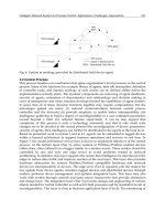
EXAMPLE 9.2–3: Stiffness Controller for a Cartesian Manipulator
We want to design and simulate a stiffness controller for the robot
manipulator system given in Figure 9.2.5. The control objective is to move
the end effector to a desired final position of v
d
=3 m while exerting a final
desired normal force of f
d1
=2 N. We neglect the surface friction (i.e., f
2
) and
joint friction, and assume that the normal force (i.e., f
1
) satisfies the
relationship
(1)
where and k
e
=1000 N/m. The robot link masses are assumed
to be unity, and the initial end-effector position is given by

(2)
To accomplish the control objective, the stiffness controller from Table 9.2.1
is given by
(3)
where

Copyright © 2004 by Marcel Dekker, Inc.
Force Control478
␶
, J, G, and x are as defined in Example 9.2.1, u
d
is defined as the desired
normal position, and the gain matrices K
v
and K
p
have been taken to be
K
v
=k
v
I and K
p
=k
p
I. For this example we select k
v
= k
p
=10, which will

guarantee that k
p
<< k
e
as required in the stiffness control formulation. To
satisfy the control objective that f
d1
=2 N, we utilize (9.2.27) to determine
the desired normal position. Specifically, substituting the values of f
d1
, k
e
,
and u
e
into
(4)
yields
The simulation of the stiffness controller given by (3) for the robot
manipulator system (Figure 9.2.5) is given in Figure 9.2.7. As indicated by
the simulation, the desired tangential position and normal force are reached
in about 4 s.
᭿
9.3 Hybrid Position/Force Control
A major disadvantage of the stiffness controller given in Section 9.2 is that it
can only be used for set-point control; in other words, the desired end effector
manipulator position and the desired force exerted on the environment must
be constant. In many robotic applications, such as grinding, the end effector
must track a desired positional trajectory along the object surface while
Figure 9.2.7: Simulation of stiffness controller.

Copyright © 2004 by Marcel Dekker, Inc.
479
tracking a desired force trajectory exerted onto the object surface. In this
type of application, a stiffness controller will not perform adequately;
therefore, another control approach must be utilized.
The so-called hybrid position/force controller [Chae et al. 1988] and
[Raibert and Craig 1981] can be used for tracking position and force
trajectories simultaneously. The basic concept of the hybrid position/force
controller is to decouple the position and force control problems into subtasks
via a task space formulation. As we have seen, the task space formulation is
valuable in determining which directions should be force or position
controlled. That is, the position and force control subtasks are easily
determined from the task space formulation. After the control subtasks have
been identified, separate position and force controllers can then be developed.
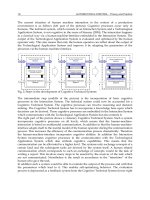
Hybrid Position/Force Control of a Cartesian Two-Link Arm
To illustrate this concept of hybrid position/force control, consider the robot
manipulator system given by Figure 9.3.1. For this application, the position
along the surface and the normal force exerted on the surface should both be
controlled; therefore, one must determine which variables should be force
controlled and which should be position controlled.
9.3 Hybrid Position/Force Control
Figure 9.3.1: Manipulator moving along perpendicular surface.
Copyright © 2004 by Marcel Dekker, Inc.
Force Control480
Following the task space concept given in Section 9.2, the task space
formulation for the manipulator system given in Figure 9.3.1 is
(9.3.1)
with the task-space Jacobian matrix given by

As illustrated by (9.3.1), the task space and the joint space are equivalent for

this problem; therefore, we will refer to joint variables as task-space variables
throughout this problem.
To design the position/force controller for the manipulator system, we
must first determine the dynamic equations for the task space formulation
given by (9.3.1). Using this task space formulation and neglecting joint
friction, the manipulator dynamics can be shown to be
(9.3.2)
where ␶, M, G, and f are as defined in Example 9.2.1. The two dynamic
equations given in the matrix form represented by (9.3.2) are
(9.3.3)
and
(9.3.4)
In formulating a hybrid position/force controller, we design separate
controllers for the dynamics given by (9.3.3) and (9.3.4). As illustrated by
Figure 9.3.1, the position along the task space direction q
2
should be position
controlled; therefore, we should use (9.3.4) for designing the position
controller. [This is obvious because the dynamics given by (9.3.3) do not
contain the task space variable q2.]
Because we are designing a position controller to track a desired trajectory,
we will define the “tangent space” tracking error to be
(9.3.5)
where q
d2
represents the desired position trajectory along or tangent to the
surface. The position controller will be the computed-torque controller (see
Chapter 3)
(9.3.6)
Copyright © 2004 by Marcel Dekker, Inc.

481
where
(9.3.7)
with k
Tv
and k
Tp
being positive control gains. Substituting (9.3.6) into (9.3.4)
gives the position tracking error system
(9.3.8)
By using the fact that k
Tv
and k
Tp
are positive, we can apply standard linear
control results to (9.3.8) to yield

therefore, asymptotic positional tracking is guaranteed with the controller
given by (9.3.6). Note that the position controller requires measurement of
the joint position, joint velocity, and surface friction force; therefore, from
an implementation point of view, force measurements are required in the
position controller.
The position controller given in (9.3.6) will ensure good position tracking
along the surface of the environment; however, we also want to control the
force exerted on the environment. For the manipulator system given in Figure
9.3.1, the task space direction normal to the surface is q
1
; therefore, we will
assume that in this direction the environment can be modeled as a spring.
Specifically, the normal force f

1
exerted on the environment is given by
(9.3.9)
where k
e
represents the environment stiffness and q
e
=3. Taking the second
derivative of (9.3.9) with respect to time gives the expression
(9.3.10)
where the normal task space acceleration is written in terms of the second
derivative of the normal force. Substituting (9.3.10) into (9.3.3) yields the
force dynamic equation
(9.3.11)
We can now use the force dynamic equation given in (9.3.11) to design a
force controller to track a desired force trajectory. First, define the force
tracking error to be
9.3 Hybrid Position/Force Control
Copyright © 2004 by Marcel Dekker, Inc.
Force Control482
(9.3.12)
where f
d1
represents the desired normal force that is to be exerted on the
environment. Similar to the position controller, the force controller will be
the computed-torque controller
(9.3.13)
where
(9.3.14)
with k

Nv
and k
Np
being positive control gains. Substituting (9.3.13) into
(9.3.11) gives the force tracking error system,
(9.3.15)
Using the fact k
Nv
and k
Np
are positive in (9.3.15) yields

therefore, asymptotic force tracking is guaranteed with the controller given
by (9.3.13). It is important to realize that the force controller requires
measurement of the normal force and the derivative of the normal force.
Because the force derivative is often not available for measurement, it is
manufactured from (9.3.9), that is,
(9.3.16)
therefore, the stiffness of the environment and the normal task space velocity
are used to simulate the derivative of the force.
Hybrid Position/Force Control of an N-Link Manipulator
The hybrid position/force controller given in the preceding section can easily
be extended to the multidegree case by using the task space formulation
concept. Specifically, one can develop a feedback-linearizing control that
will globally linearize the robot manipulator equation and then develop linear
controllers to track the desired force and position trajectories.
First, the control designer selects a task space formulation
(9.3.17)
Copyright © 2004 by Marcel Dekker, Inc.
483

such that the normal and tangent surface motions are decomposed as
discussed in Section 9.2. The robot dynamics given in (9.3.14) are then written
in terms of the task space acceleration by differentiating (9.3.17) twice with
respect to time to obtain
(9.3.18)
where J(q) is the task space Jacobian defined in (9.2.11). Solving (9.3.18) for
q yields
(9.3.19)
Substituting (9.3.19) into (9.2.14) yields
(9.3.20)
The corresponding feedback linearizing control for the dynamics given by
(9.3.20) is given by
(9.3.21)
where a is an n×1 vector used to represent the linear position and force
control strategies, which will be discussed later. After substituting (9.3.21)
into (9.3.20), we have
(9.3.22)
From (9.3.22), we can see that the task space motion has been globally
linearized and decoupled; therefore, we can design the position and force
controllers independently in a method similar to that of the preceding section.
Specifically, linear position controllers can be designed for the task space
variables that represent tangent motion; moreover, linear force controllers
can be designed for the task space variables that represent normal force.
Because the dynamics given in (9.3.20) have been decoupled in the task
space, we will define the tangent space components of x as x
Ti
, where the
subscript T is used to denote the tangent space, and the subscript i is used to
denote the ith component of x
T

. From this notation the tangent space
components of (9.3.22) are given as
(9.3.23)
9.3 Hybrid Position/Force Control
Copyright © 2004 by Marcel Dekker, Inc.
Force Control484
where a
Ti
is the ith linear tangent space position controller. For the purpose
of feedback control, we define the tangent space tracking error to be
(9.3.24)
where x
Tdi
represents the ith desired position trajectory tangent to the
environment surface. As in the preceding section, the corresponding linear
controller is then given as
(9.3.25)
with k
Tvi
and k
Tpi
being the ith positive control gains. Substituting (9.3.25)
into (9.3.23) gives the position tracking error system
(9.3.26)
Using the fact that k
Tvi
and k
Tpi
are positive in (9.3.26) yields

therefore, asymptotic positional tracking is guaranteed.
For purposes of force control, we define the normal space components of
x as x
Nj
where the subscript N is used to denote normal space, and the subscript
j is used to denote the jth component of x
N
. From this notation, the normal
space components of (9.3.22) are given as
(9.3.27)
where a
Nj
is the jth linear normal space force controller. As in the preceding
section, we assume that the environment can be modeled as a spring.
Specifically, the normal force f
Nj
exerted on the environment is given by
(9.3.28)
where k
ej
is the jth component of environmental stiffness, and x
ej
is used to
represent the static location of the environment in the direction of the normal
space x
Nj
.
As done for the single-degree-of-freedom robot in the preceding subsection,
we must formulate the force dynamics before we can develop the force
controller. Taking the second derivative of (9.3.28) with respect to time gives

the expression
(9.3.29)
Copyright © 2004 by Marcel Dekker, Inc.
485
where the normal task space acceleration is written in terms of the second
derivative of the normal force. Substituting (9.3.29) into (9.3.27) yields the
force dynamics
(9.3.30)
For the purpose of feedback control, we define the force tracking error to be
(9.3.31)
where f
Ndj
represents the jth component of the desired force exerted normal
to the environment. As in the preceding section, the corresponding linear
controller is then given by
(9.3.32)
with k
Nvj
and k
Npj
being the jth positive control gains. Substituting (9.3.32)
into (9.3.30) gives the force tracking error system
(9.3.33)
Using the fact that k
Nvj
and k
Npj
are positive in (9.3.33) yields

therefore, asymptotic force tracking is guaranteed.

The hybrid position/force controller and the corresponding stability result
are both summarized in Table 9.3.1. We now illustrate the concept of hybrid
position/force control with an example.
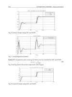
EXAMPLE 9.3–1: Hybrid Position/Force Control Along a Slanted Surface
We want to design and simulate a hybrid position/force controller for the
robot manipulator system given in Figure 9.2.5. The control objective is
to move the end effector with a desired surface trajectory of v
d
=sin(t) m
while exerting a normal force trajectory of . We neglect
joint friction and assume that the normal force (i.e., f
1
) satisfies the
relationship
(1)
9.3 Hybrid Position/Force Control
Copyright © 2004 by Marcel Dekker, Inc.
487
given by (3) decouples the robot dynamics in the task space as follows:
(4)
From Figure 9.2.5, we can see that the task space variable u represents the
normal space, and the task space variable v represents the tangent space;
therefore, (4) may rewritten in the notation given in Table 9.3.1 as
(5)
From Table 9.3.1, the corresponding linear position and force controllers
are then given by
(6)
and
(7)
where , and k

e1
=1000.
The simulation of the hybrid position/force controller given by (3), (6),
and (7) for the robotic manipulator system (Figure 9.2.5) is given in Figure
9.3.2. The controller gains were selected as

As indicated by the simulation, the position and force tracking error go to
zero in about 4 s.
᭿
Implementation Issues
After reexamining the hybrid position/force controller, one can see that the
task space forces are needed for implementation of the control law. Often
a wrist-mounted force sensor is used for measuring the end-effector forces;
however, in general, these forces will not be the task space forces that are
needed for control implementation. Fortunately, a transformation can be
9.3 Hybrid Position/Force Control
Copyright © 2004 by Marcel Dekker, Inc.
489
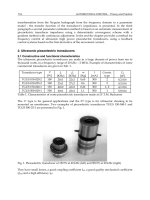
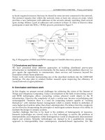
With these implementational concerns in mind, the overall hybrid position/
force control strategy is depicted in Figure 9.3.3. The feedforward terms in
the block diagram are used to represent the terms
(9.3.37)
in the control law given in Table 9.3.1.
9.4 Hybrid Impedance Control
Impedance control is based on the concept that the controller should be used
to regulate the dynamic behavior between the robot manipulator motion
and the force exerted on the environment [Hogan 1987] rather than
considering the motion and force control problems separately. Using this
concept, the control designer specifies the desired dynamic behavior between
the motion of the manipulator and the force exerted on the environment.

This desired behavior is sometimes referred to as the target impedance because
it is used to represent an Ohm’s law type of relationship between motion and
force.
9.4 Hybrid Impedance Control
Figure 9.3.3: Hybrid position/force controller.
Copyright © 2004 by Marcel Dekker, Inc.
Force Control490
Modeling the Environment
As pointed out in [Hogan 1987], the environmental model is central to any
force control strategy. In the force control strategies discussed previously,
the environment has simply been modeled as a spring; however, as one might
imagine, a simple spring model may not adequately describe all types of
environments. To classify the many types of environments, we use the linear
transfer function relationship
(9.4.1)
where the variable s is the Laplace transform variable, f represents the force
exerted on the environment, x represents the velocity of the manipulator at
the environmental contact point, and Z
e
(s) represents the environmental
impedance. For now, all quantities are assumed to be scalar functions;
however, at the end of this section we generalize impedance control to the
multidimensional case.
The quantity Z
e
(s) is called an impedance because (9.4.1) represents an
Ohm’s law type of relationship between motion and force. As in circuit theory,
environmental impedances can be separated into different categories. To
further our impedance control discussion, we now give three commonly used
categories which are used to classify environmental impedances.

DEFINITION 9.4–1 An impedance is inertial if and only if |Z(0)|=0.
᭿
An illustration of an inertial environment is given in Figure 9.4.1a. This
figure depicts a robot manipulator moving a payload of mass h with velocity
x. The corresponding interaction force is given by

therefore, utilizing (9.4.1) yields an inertial environmental impedance of
(9.4.2)
We can easily verify that this impedance is indeed inertial by applying
Definition 9.4.1.
DEFINITION 9.4–2 An impedance is resistive if and only if |Z(0)|=c where
0<c<ϱ. ᭿
An illustration of a resistive environment is given in Figure 9.4.1b. This figure
depicts a robot manipulator moving through a liquid medium with velocity x.
Copyright © 2004 by Marcel Dekker, Inc.
Force Control492
DEFINITION 9.4–3 An impedance is capacitive if and only if |Z(O)|= ϱ.
᭿
An illustration of a capacitive environment is given in Figure 9.4.1c.
This figure depicts a robot manipulator pushing against an object of
mass h with velocity x. The object is assumed to have a damping
coefficient of b and a spring constant of k. The corresponding interaction
force is given by

therefore, utilizing (9.4.1) yields a capacitive environmental impedance of
(9.4.4)
We can easily verify that this impedance is indeed capacitive by applying
Definition 9.4.3.
Position and Force Control Models
As we have seen in the preceding section, the environment can be modeled as

an impedance defined by the force/velocity relationship in (9.4.1). For our
impedance control formulation, we will assume that the environmental
impedance is either inertial, resistive, or capacitive. The question then
becomes: How does one design a controller for a given environmental
impedance? The solution is obtained by formulating a manipulator impedance
model, Zm(s) [Anderson and Spong 1988]. In other words, a manipulator
impedance (or target impedance) is selected after the environment has been
modeled. The criterion for selecting the manipulator impedance is related to
the dynamic performance of the manipulator. That is, the manipulator
impedance is selected such that there is zero steadystate error to a step input
(which may be a force or velocity command). As we will show, this
performance criterion can be achieved if the manipulator impedance is the
dual of the environmental impedance.
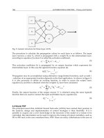
Before the concept of duality can be illustrated fully, the models for position
and force control must be formulated. For position control [Anderson and
Spong 1988], the relationship between force and velocity is modeled by
(9.4.5)
where x
d
represents the input velocity of the manipulator at the environmental
contact point and Z
m
(s) represents the manipulator impedance.
Copyright © 2004 by Marcel Dekker, Inc.
493
As we will show subsequently, the manipulator impedance Z
m
(s) is selected
to “zero-out” the steady state to a step input by utilizing the dynamic
relationship between x and x

d
, To determine the dynamic relation between x
and x
d
. we combine (9.4.1) with (9.4.5) to yield the position control block
diagram given in Figure 9.4.2. We can use this block diagram to illustrate
the concept of duality. Specifically, we examine the steady-state velocity error
(9.4.6)
where for a step velocity input. Utilizing Figure 9.4.2, we can
easily show that (9.4.6) can be reduced to
(9.4.7)
For E
ss
to be equal to zero in (9.4.7), Z
e
(s) must be a noncapacitive impedance
[i.e., Z
e
(s) must be inertial or resistive], and Z
m
(s) must be a noninertial
impedance. That is, zero steady-state error can be achieved for a velocity
step input if inertial environments are position controlled with noninertial
manipulator impedances, while resistive environments are position controlled
with capacitive manipulator impedances. The aforementioned term duality
is used to emphasize the fact that inertial environmental impedances can be
position controlled with capacitive manipulator impedances.
9.4 Hybrid Impedance Control
From the development above, it is obvious that a capacitive environment
cannot be position controlled and maintain the zero steady-state error

specification. However, subsequently we will show that capacitive
environments can be force controlled while maintaining the zero steady-
state error specification. With regard to force control, the dynamic relationship
between force and velocity is modeled [Anderson and Spong 1988] by
(9.4.8)
Figure 9.4.2: Position control block diagram.
Copyright © 2004 by Marcel Dekker, Inc.
Force Control494
where f
d
is used to represent the input force exerted at the environmental
contact point.
As we will show subsequently, the manipulator impedance Z
m
(s) is selected
to “zero-out” the steady state to a step input by utilizing the dynamic
relationship between f and f
d
. To determine the dynamic relation between f
and f
d
, we combine (9.4.1) with (9.4.8) to yield the force control block diagram
given in Figure 9.4.3. We can use this block diagram to illustrate the concept
of duality. Specifically, we examine the steady-state force error
(9.4.9)
where f
d
(s)=1/s for a step force input. Utilizing Figure 9.4.3, we can easily
show that (9.4.9) can be reduced to
(9.4.10)

For E
ss
to be equal to zero in (9.4.10), Z
e
(s) must be a noninertial impedance,
and Z
m
(s) must be a noncapacitive impedance. That is, zero steady-state
error can be achieved for a force step input if capacitive environments are
force controlled with noncapacitive manipulator impedances while resistive
environments are force controlled with inertial manipulator impedances.
The term “duality” is used to emphasize the fact that capacitive
environmental impedances can be force controlled with inertial manipulator
impedances.
The discussion above can be summarized by the following duality
principle.
DUALITY PRINCIPLE Capacitive environments are force controlled with
noncapacitive manipulator impedances, inertial environments are position
controlled with noninertial manipulator impedances, and resistive
environments are force controlled with inertial manipulator impedances or
position controlled with capacitive manipulator impedances.
Impedance Control Formulation
Now that we have illustrated how the environment and the manipulator can
be modeled as impedances, we develop an “impedance” controller based on
this model. To utilize an impedance control approach, the control designer
selects a task space formulation
(9.4.11)
Copyright © 2004 by Marcel Dekker, Inc.
Force Control496
(9.4.15)

From the position control model given by (9.4.5), we can also write the left-
hand side of (9.4.15) as
(9.4.16)
where Z
pmi
is the ith position-controlled manipulator impedance. Therefore,
equating (9.4.16) and (9.4.15) gives the ith position controller
(9.4.17)
where L
-1
is used to represent the inverse Laplace transform operation.
Continuing with the separation of position and force control designs, we
use (9.4.13) to define the equations that are to be force controlled in the task
space directions as
(9.4.18)
where the subscript j denotes the jth force-controlled task space variable,
and the subscript f denotes force control. The associated environmental forces
in the force-controlled task space directions are denoted by f
fj
.
Assuming zero initial conditions, the Laplace transform of (9.4.18) can
be written as:
(9.4.19)
From the force control model given in (9.4.8), the left-hand side of (9.4.19)
can also be written as
(9.4.20)
(9.4.21)
where Z
fmj
is the jth force-controlled manipulator impedance. Therefore,

equating (9.4.21) and (9.4.19) gives the jth force controller
The overall “hybrid” impedance control strategy is obtained by using
(9.4.12) in conjunction with (9.4.17) and (9.4.20). This hybrid impedance
control strategy is summarized in Table 9.4.1. Note that a higher-level
controller would be used to select the components of the task space which
Copyright © 2004 by Marcel Dekker, Inc.
Force Control498
(2)
where h
e
, b
e
, d
e
, and k
e
are all positive scalar constants.
From Table 9.4.1, the hybrid impedance controller is given by
(3)
where a is a 2×1 vector representing the separate position and force control
strategies, and ␶, J, G, and f are as defined in Example 9.2.1. The torque
controller given by (3) decouples the robot dynamics in the task space as
follows:
(4)
therefore, we can easily determine which task space directions should be
force or position controlled.
Applying Definition 9.4.2 to (1) allows us to state that the environmental
impedance in the task space direction given by v is a resistive impedance;
therefore, by the duality principle, we will select a position controller that
utilizes the capacitive manipulator impedance

(5)
where h
m
, b
m
, and k
m
are all positive scalar constants. Since the task space
variable v will be position controlled, we use the notation from (9.4.14) to
yield

and

Now using (5) and the definition of a
p1
given in Table 9.4.1, we can easily
show that
(6)
Copyright © 2004 by Marcel Dekker, Inc.
499
Applying Definition 9.4.3 to (2) allows us to state that the environmental
impedance in the task space direction given by u is capacitive; therefore, by
the duality principle, we will select a force controller that utilizes the inertial
manipulator impedance
(7)
where d
m
is a positive scalar constant. Since the task space variable u will be
force controlled, we use the notation from (9.4.18) to yield

and

Using (7) and the definition of a f
1
given in Table 9.4.1, we can easily show
that
(8)
The overall impedance control strategy is obtained by substituting
(9)
into (3), where a
p1
and a
f1
are as given by (6) and (8), respectively.
᭿
Implementation Issues
As mentioned earlier, the manipulator impedance Z
m
(s) is selected such
that the duality principle is maintained. However, from a practical point of
view, Z
m
(s) should also be selected in the expressions for a
pi
and a
fj
such
that only measurements of f, x, and x are required. In other words, our
controller should not require acceleration (i.e., x) or force derivative (i.e.,
f) measurements. We can easily show that the expressions for a

pi
and a
fj
will not require measurements of f and x if the manipulator impedance is
selected as

9.4 Hybrid Impedance Control
Copyright © 2004 by Marcel Dekker, Inc.