The MEMS Handbook Introduction & Fundamentals (2nd Ed) - M. Gad el Hak Part 14 doc

15
Model-Based Flow
Control for
Distributed
Architectures
15.1 Introduction 15-2
15.2 Linearization: Life in a Small Neighborhood 15-3
15.3 Linear Stabilization: Leveraging Modern Linear
Control Theory 15-6
The H
∞
Approach to Control Design • Advantages of Modern
Control Design for Non-Normal Systems • Effectiveness of
Control Feedback at Particular Wavenumber Pairs
15.4 Decentralization: Designing for Massive Arrays 15-14
Centralized Approach • Decentralized Approach
15.5 Localization: Relaxing Nonphysical Assumptions 15-16
Open Questions
15.6 Compensator Reduction: Eliminating Unnecessary
Complexity 15-18
Fourier-Space Compensator Reduction • Physical-Space
Compensator Reduction • Nonspatially Invariant Systems
15.7 Extrapolation: Linear Control of Nonlinear Systems 15-20
15.8 Generalization: Extending to Spatially Developing
Flows 15-23
15.9 Nonlinear Optimization: Local Solutions for Full
Navier–Stokes 15-25
Adjoint-Based Optimization Approach • Continuous Adjoint
vs. Discrete Adjoint
15.10 Robustification: Appealing to Murphy’s Law 15-33
We ll-Posedness • Convergence of Numerical Algorithms

15.11 Unification: Synthesizing a General Framework 15-35
15.12 Decomposition: Simulation-Based System
Modeling 15-35
15.13 Global Stabilization: Conservatively Enhancing
Stability 15-36
15.14 Adaptation: Accounting for a Changing
Environment 15-37
15-1
© 2006 by Taylor & Francis Group, LLC
15.15 Performance Limitation: Identifying Ideal Control
Targets 15-37
15.16 Implementation: Evaluating Engineering
Trade-Offs 15-38
15.17 Discussion: A Common Language for Dialog 15-40
15.18 The Future: A Renaissance 15-40
As traditional scientific disciplines individually grow toward their maturity, many new opportunities for
significant advances lie at their intersection. For example, remarkable developments in control theory in
the last few decades have considerably expanded the selection of available tools which may be applied to
regulate physical and electrical systems. When combined with microelectromechanical systems (MEMS)
techniques for distributed sensing and actuation, as highlighted elsewhere in this handbook, these tech-
niques hold great promise for several applications in fluid mechanics, including the delay of transition and
the regulation of turbulence. Such applications of control theory require a very balanced perspective in
which one considers the relevant flow physics when designing the control algorithms and, conversely, takes
into account the requirements and limitations of control algorithms when designing both reduced-order
flow models and the fluid-mechanical systems to be controlled. Such a balanced perspective is elusive,
however, as both the research establishment in general and universities in particular are accustomed only
to the dissemination and teaching of component technologies in isolated fields. To advance, we must not
toss substantial new interdisciplinary questions over the fence for fear of them being “outside our area;”
rather, we must break down these very fences that limit us and attack these challenging new questions with
a Renaissance approach. In this spirit, this chapter surveys a few recent attempts at bridging the gaps

between the several scientific disciplines comprising the field of flow control, in an attempt to clarify the
author’s perspective on how recent advances in these constituent disciplines fit together in a manner that
opens up significant new research opportunities.
15.1 Introduction
Flow control is perhaps the most difficult grand challenge application area for MEMS technology.
Potentially, it is one of the most rewarding because a common feature in many fluid systems is the existence
of natural instability mechanisms by which a small input, when coordinated correctly, can lead to a large
response in the overall system. As one of the key driving application areas for MEMS, it is appropriate to
survey recent developments in the fundamental framework for flow control in this handbook.
The area of flow control plainly resides at the intersection of disciplines, incorporating essential and
nontrivial elements from control theory, fluid mechanics, Navier–Stokes mathematics, numerical methods,
and fabrication technology for “small”(millimeter-scale), self-contained, durable devices which can integrate
the functions of sensing, actuation, and control logic. Recent developments in the integration of these dis-
ciplines, while grounding us with appropriate techniques to address some fundamental open questions,
hint at the solution of several new questions. To follow up on these new directions, it is essential to have a
clear vision of how recent advances in these fields fit together and to know where the significant unresolved
issues at their intersection lie.
This chapter attempts to elucidate the utility of an interdisciplinary perspective to this type of problem
by focusing on the control of a prototypical and fundamental fluid system: plane channel flow. The control
of the flow in this simple geometry embodies a myriad of complex issues and interrelationships. These issues
and relationships require us to draw from a variety of traditional disciplines. Only when these issues and
perspectives are combined is a complete understanding of the state of the art achieved and a vision of where
to proceed identified.
15-2 MEMS: Introduction and Fundamentals
Thomas R. Bewley
University of California
© 2006 by Taylor & Francis Group, LLC
Though plane channel flow will be the focus problem we discuss here, the purpose of this work goes well
beyond simply controlling this particular flow with a particular actuator/sensor configuration. At its core, the
research effort we describe is devoted to the development of an integrated, interdisciplinary understanding

that allows us to synthesize the necessary tools to attack a variety of flow control problems in the future.
The focus problem of control of channel flow is chosen not simply because of its technological relevance
or fundamental character, but because it embodies many of the important unsolved issues encountered in the
assortment of new flow control problems that will inevitably follow. The primary objective of this work is
to lay a solid, integrated footing upon which these future efforts may be based.
To this end, this chapter will describe mostly the efforts with which the author has been directly involved,
in an attempt to weave the story that threads these projects together as part of the fabric of a substantial
new area of interdisciplinary research. Space does not permit complete development of these projects;
rather, the chapter will survey a selection of recent results that bring the relevant issues to light. Refer to the
appropriate full journal articles for all of the relevant details and careful placement of these projects in
context with the works of others. Space limitations also do not allow this brief chapter to adequately
review the various directions all my friends and colleagues are taking in this field. Rather than attempt such
areview and fail, refer to a host of other recent reviews which span only a fraction of the current work being
done in this active area of research. For an experimental perspective, refer to several other chapters in this
handbook and to the recent reviews of Ho and Tai (1996, 1998), McMichael (1996), Gad-el-Hak (1996),
and Löfdahl and Gad-el-Hak (1999). For a mathematical perspective, refer to the recent dedicated volumes
compiled by Banks (1992), Banks et al. (1993), Gunzburger (1995), Lagnese et al. (1995), and Sritharan
(1998) for a sampling of recent results in this area.
15.2 Linearization: Life in a Small Neighborhood
As a starting point for the introduction of control theory into the fluid-mechanical setting, we first con-
sider the linearized system arising from the equation governing small perturbations to a laminar flow.
From a physical point of view, such perturbations are quite significant because they represent the initial
stages of the complex process of transition to turbulence. Therefore, their mitigation or enhancement has
a substantial effect on the evolution of the flow.
An enlightening problem that captures the essential physics of many important features of both tran-
sition and turbulence in wall-bounded flows is that of plane channel flow, as illustrated in Figure 15.1.
Assume the walls are located at y ϭ Ϯ1. We begin our study by analyzing small perturbations {u, v, w, p}
to the (parabolic) laminar flow profile U(y) in this geometry, which are governed by the linearized incom-
pressible Navier–Stokes equation:
ϩ ϩ ϭ 0, (15.1a)

u
·
ϩ U uϩ UЈv ϭ Ϫ ϩ ∆u, (15.1b)
v
·
ϩ U v ϭ Ϫ ϩ ∆v, (15.1c)
w
·
ϩ U w ϭ Ϫ ϩ ∆w. (15.1d)
Equation (15.1a), the continuity equation, constrains the solution of Equations (15.1b) to (15.1d), the
momentum equations, to be divergence free. This constraint is imposed through the ∇p terms in the
momentum equations, which act as Lagrange multipliers to maintain the velocity field on a divergence-free
submanifold of the space of square-integrable vector fields. In the discretized setting, such systems are
1
ᎏ
Re
∂p
ᎏ
∂z
∂
ᎏ
∂x
1
ᎏ
Re
∂p
ᎏ
∂y
∂
ᎏ

∂x
1
ᎏ
Re
∂p
ᎏ
∂x
∂
ᎏ
∂x
∂w
ᎏ
∂z
∂v
ᎏ
∂y
∂u
ᎏ
∂x
Model-Based Flow Control for Distributed Architectures 15-3
© 2006 by Taylor & Francis Group, LLC
called descriptor systems or differential-algebraic equations and, defining a state vector x and a control
vector u, may be written in the generalized state-space form:
Ex
·
ϭ Ax ϩ Bu. (15.2)
If the Navier–Stokes Equation (15.1) is put directly into this form, E is singular. This is an essential fea-
ture of the Navier–Stokes equation that necessitates careful treatment in both simulation and control
design to avoid spurious numerical artifacts. A variety of techniques exist to express the system of
Equations (15.1) with a reduced set of variables or spatially distributed functions with only two degrees

of freedom per spatial location, referred to as a divergence-free basis. In such a basis, the continuity equa-
tion is applied implicitly, and the pressure is eliminated from the set of governing equations. All three
velocity components and the pressure (up to an arbitrary constant) may be determined from solutions
represented in such a basis. When discretized and represented in the form of Equation (15.2), the
Navier–Stokes equation written in such a basis leads to an expression for E that is nonsingular.
For the geometry indicated in Figure 15.1, a suitable choice for this reduced set of variables, which is
convenient in terms of the implementation of boundary conditions, is the wall-normal velocity v and the
wall-normal vorticity,
ω
ϭ
∆
∂u/∂z Ϫ ∂w/∂x. Taking the Fourier transform of Equation (15.1) in the stream-
wise and spanwise directions and manipulating these equations and their derivatives leads to the classical
Orr–Sommerfeld/Squire formulation of the Navier–Stokes equation at each wavenumber pair {k
x
, k
z
}:
∆
ˆ
v
ˆ
·
ϭ {Ϫik
x
U∆
ˆ
ϩ ik
x
UЉ ϩ ∆

ˆ
(∆
ˆ
/Re)}vˆ , (15.3a)
ω
ˆ
·
ϭ {Ϫik
z
UЈ}vˆ ϩ {Ϫik
x
U ϩ ∆
ˆ
/Re}
ω
ˆ
, (15.3b)
where the hats (ˆ) indicate Fourier coefficients and the Laplacian now takes the form ∆
ˆ
ϭ
∆
∂
2
/∂y
2
Ϫ k
2
x
Ϫ k
2

z
.
Particular care is needed when solving this system; to invert the Laplacian on the LHS of Equation
15-4 MEMS: Introduction and Fundamentals
FIGURE 15.1 Geometry of plane channel flow. The flow is sustained by an externally applied pressure gradient in
the x direction. This canonical problem provides an excellent testbed for the study of both transition and turbulence
in wall-bounded flows. Many of the important flow phenomena in this geometry, in both the linear and nonlinear
setting, are fundamentally three dimensional. A nonphysical assumption of periodicity of the flow perturbations in
the x and z directions is often assumed for numerical convenience, with the box size chosen to be large enough that
this nonphysical assumption has minimal effect on the observed flow statistics. It is important to evaluate critically the
implications of such assumptions during the process of control design, as discussed in detail in Sections 15.4 and 15.5.
© 2006 by Taylor & Francis Group, LLC
(15.3a), the boundary conditions on v must be accounted for properly. By manipulating the governing
equations and casting them in a derivative form, we effectively trade one numerical difficulty (singular-
ity of E) for another (a tricky boundary condition inclusion to make the Laplacian on the LHS of
Equation (15.3a) invertible).
Note the spatially invariant structure of the present geometry: every point on each wall is, statistically
speaking, identical to every other point on that wall. Canonical problems with this sort of spatially invari-
ant structure in one or more directions form the backbone of much of the literature on flow transition
and turbulence. It is this structure that facilitates the use of Fourier transforms to completely decouple
the system state {vˆ,
ω
ˆ
} at each wavenumber pair {k
x
, k
z
} from the system state at every other wavenumber
pair, as indicated in Equation (15.3). Such decoupling of the Fourier modes of the unforced linear system
in the directions of spatial invariance is a classical result upon which much of the available linear theory

for the stability of Navier–Stokes systems is based. As noted by Bewley and Agarwal (1996), taking the
Fourier transform of both the control variables and the measurement variables maintains this system
decoupling in the control formulation, greatly reducing the complexity of the control design problem to
several smaller, completely decoupled control design problems at each wavenumber pair {k
x
, k
z
}, each of
which requires spatial discretization in the y direction only.
Once a tractable form of the governing equation has been selected, to pose the flow control problem
completely, several steps remain:
●
the state equation must be spatially discretized,
●
boundary conditions must be chosen and enforced,
●
the variables representing the controls and the available measurements must be identified and
extracted,
●
the disturbances must be modeled, and
●
the “control objective” must be precisely defined.
To identify a fundamental yet physically relevant flow control problem, the decisions made at each of
these steps require engineering judgment. Such judgment is based on physical insight concerning the flow
system to be controlled and how the essential features of such a system may be accurately modeled. An
example of how to accomplish these steps is described in some detail by Bewley and Liu (1998). In short,
we may choose:
●
a Chebyshev spatial discretization in y,
●

no-slip boundary conditions (u ϭ w ϭ 0 on the walls) with the distribution of v on the walls (the
blowing/suction profile) prescribed as the control,
●
skin friction measurements distributed on the walls,
●
idealized disturbances exciting the system, and
●
an objective of minimizing flow perturbation energy.
As we learn more about the physics of the system to be controlled, there is significant room for improve-
ment in this problem formulation, particularly in modeling the structure of relevant system disturbances
and in the precise statement of the control objective.
Once the previously mentioned steps are complete, the present decoupled system at each wavenumber
pair {k
x
, k
z
} may finally be manipulated into the standard state-space form:
x
·
ϭ Ax ϩ B
1
w ϩ B
2
u, (15.4)
y ϭ C
2
x ϩ D
21
w,
with

B
1
ϭ
∆
(G
1
0), C
2
ϭ
∆
G
2
Ϫ1
C, D
21
ϭ
∆
(0
α
I), w
ϭ
∆
΂ ΃
,
where x denotes the state, u denotes the control, y denotes the available measurements (scaled as dis-
cussed below), and w accounts for the external disturbances (including the state disturbances w
1
and the
w
1

w
2
Model-Based Flow Control for Distributed Architectures 15-5
© 2006 by Taylor & Francis Group, LLC
measurement noise w
2
, scaled as discussed below). Note that Cx denotes the raw vector of measured vari-
ables, and G
1
and
α
G
2
represent the square root of any known or expected covariance structure of the
state disturbances and measurement noise, respectively. The scalar
α
2
is identified as an adjustable
parameter that defines the ratio of the maximum singular value of the covariance of the measurement noise
divided by the maximum singular value of the covariance of the state disturbances; without loss of gen-
erality, we take
σ
–
(G
1
) ϭ
σ
–
(G
2

) ϭ 1. Effectively, the matrix G
1
reflects which state disturbances are strongest,
and the matrix G
2
reflects which measurements are most corrupted by noise. Small a implies relatively
highoverallconfidence in the measurements, whereas large
α
implies relatively low overall confidence in
the measurements.
Not surprisingly, there is a wide body of theory surrounding how to control a linear system in the standard
form of Equation (15.4). The application of one popular technique (to a related two-dimensional problem),
called proportional–integral (PI) control and generally referred to as “classical” control design, is presented
in Joshi et al. (1997). The application of another technique, called H
ϱ
control and generally referred to as
“modern” control design, is laid out in Bewley and Liu (1998). The application of arelated modern control
strategy (to the two-dimensional problem), called loop transfer recovery (LTR), is presented in Cortelezzi
and Speyer (1998). More recent publications by these groups further extend these seminal efforts.
It is useful to understand the various theoretical implications of the control design technique chosen.
Ultimately, however, flow control is the design of acontrol that achieves the desired engineering objective
(transition delay, drag reduction, mixing enhancement, etc.) to the maximum extent possible. The theo-
retical implications of the particular control technique chosen are useful only to the degree to which they
help attain this objective. Engineering judgment, based on an understanding of the merits of the various
control theories and based on the suitability of such theories to the structure of the fluid-mechanical
problem of interest, guides the selection of an appropriate control design strategy. In the following sec-
tion, we summarize the H
∞
control design approach, illustrate why this approach is appropriate for the
structure of the problem at hand, and highlight an important distinguishing characteristic of the present

system when controls computed via this approach are applied.
15.3 Linear Stabilization: Leveraging Modern Linear
Control Theory
As only a limited number of noisy measurements y of the state x are available in any practical control
implementation, it is beneficial to develop a filter that extracts as much useful information as possible
from the available flow measurements before using this filtered information to compute a suitable con-
trol. In modern control theory, a model of the system itself is used as this filter, and the filtered informa-
tion extracted from the measurements is simply an estimate of the state of the physical system. This
intuitive framework is illustrated schematically in Figure 15.2.By modeling (or neglecting) the influence
of the unknown disturbances in Equation (15.4), the system model takes the form:
xˆ
·
ϭ Axˆ ϩ B
1
w
ˆ
ϩ B
2
u Ϫ v, (15.5a)
y
ˆ
ϭ C
2
x
ˆ
ϩ D
21
w
ˆ
, (15.5b)

where x
ˆ
is the state estimate, w
ˆ
is a disturbance estimate, and v is a feedback term based on the difference
between the measurement of the state y and the corresponding quantity in the model, y
ˆ
, such that:
v ϭ L(y Ϫ y
ˆ
). (15.5c)
The control u, in turn, is based on the state estimate x
ˆ
such that:
u ϭ Kx
ˆ
. (15.6)
15-6 MEMS: Introduction and Fundamentals
© 2006 by Taylor & Francis Group, LLC
Equation (15.4) is referred to as the “plant,” Equation (15.5) is referred to as the “estimator,” and Equation
(15.6) is referred to as the “controller.” The estimator and the controller, taken together, will be referred
to as the “compensator.” The problem at hand is to compute linear time-invariant (LTI) matrices K and
L and some estimate of the disturbance, w
ˆ
, such that:
1. the estimator feedback v forces x
ˆ
toward x, and
2. the controller feedback u forces x toward zero,
even as unknown disturbances w both disrupt the system evolution and corrupt the available measure-

ments of the system state.
15.3.1 The H
∞∞
Approach to Control Design
Several textbooks describe in detail how the H
∞
technique determines K, L, and w
ˆ
for systems of the form
Equations (15.4) to (15.6) in the presence of structured and unstructured disturbances w. Refer to the
seminal paper by Doyle et al. (1989), the more accessible textbook by Green and Limebeer (1995), and
the more advanced texts by Zhou et al. (1996) and Zhou and Doyle (1998) for derivation and further dis-
cussion of these control theories. Refer to Bewley and Liu (1998) for an extended discussion in the con-
text of the present problem. To summarize this approach briefly, a cost function J describing the control
problem at hand is defined that weighs together the state x, the control u, and the disturbance w such that:
J
ϭ
∆
E[x*Qx ϩ
ᐉ
2
u*u Ϫ
γ
2
w*w]
ϭ
∆
E[z*z Ϫ
γ
2

w*w], (15.7a)
where
z
ϭ
∆
C
1
x ϩ D
12
u, C
1
ϭ
∆
΂ ΃
, D
12
ϭ
∆
΂ ΃
. (15.7b)
The matrix Q, shaping the dependence on the state in the cost function x*Qx, may be selected to numer-
ically approximate any of a variety of physical properties of the flow, such as the flow perturbation energy,
0
ᐉI
Q
1/2
0
Model-Based Flow Control for Distributed Architectures 15-7
FIGURE 15.2 Flow of information in a modern control realization. The plant, forced by external disturbances, has
an internal state x which cannot be observed. Instead, a noisy measurement y is made, with which a state estimate x

ˆ
is determined. This state estimate is then used to determine the control u to be applied to the plant to regulate x to
zero. Essentially, the full equation for the plant (or a reduced model thereof) is used in the estimator as a filter to
extract useful information about the state from the available measurements.
© 2006 by Taylor & Francis Group, LLC
its enstrophy, the mean square of the drag measurements, etc. The matrix Q may also be biased to place
extra penalty on flow perturbations in a specific region in space of particular physical significance. The
choice of Q has a profound effect on the final closed-loop behavior, and it must be selected with care.
Based on our numerical tests to date, cost functions related to the energy of the flow perturbations have
been the most successful for the purpose of transition delay. To simplify the algebra that follows, we have
set the matrices R and S shaping the u*Ru and w*Sw terms in the cost function equal to I. As shown in
Lauga and Bewley (2000), it is straightforward to generalize this result to other positive-definite choices
for R and S. Such a generalization is particularly useful when designing controls for a discretization of a
partial differential equation (PDE) in a consistent manner such that the feedback kernels converge to con-
tinuous functions as the computational grid is refined.
Given the structure of the system defined in Equations (15.4) to (15.6) and the control objective
defined in Equation (15.7), the H
∞
compensator is determined by simultaneously minimizing the cost
function J with respect to the control u and maximizing J with respect to the disturbance w. In such a
way, a control u is found that maximally attains the control objective even in the presence of a disturbance
w that maximally disrupts this objective. For sufficiently large
γ
and a system that is both stabilizable and
detectable via the controls and measurements chosen, this results in finite values for u, v, and w, the mag-
nitudes of which may be adjusted by variation of the three scalar parameters
ᐉ
,
α
, and

γ
, respectively.
Reducing
ᐉ
, modeling the “price of the control” in the engineering design, generally results in increased
levels of control feedback u. Reducing
α
, modeling the “relative level of corruption” of the measurements
by noise, generally results in increased levels of estimator feedback v. Reducing
γ
, modeling the “price”
of the disturbance to nature (in the spirit of a noncooperative game), generally results in increased
levels of disturbances w of maximally disruptive structure to be accounted for during the design of the
compensator.
The H
∞
control solution [Doyle et al., 1989] may be described as follows: a compensator that mini-
mizes J in the presence of that disturbance which simultaneously maximizes J is given by:
K
ϭ
Ϫ B*
2
X, L
ϭ
Ϫ ZYC *
2
, w
ˆ
ϭ B *
1

Xx
ˆ
, (15.8)
where
X ϭ Ric
΂
A B
1
B*
1
Ϫ B
2
B*
2
΃
,
ϪC *
1
C
1
ϪA*
Y ϭ Ric
΂
A* C*
1
C
1
Ϫ C*
2
C

2
΃
,
ϪB
1
B*
1
ϪA
Z ϭ
΂
1 Ϫ
΃
Ϫ1
,
where Ric (и) denotes the positive-definite solution of the associated Riccati equation [Laub, 1991]. The
simple structure of the above solution, and its profound implications in terms of the performance and
robustness of the resulting closed-loop system, is one of the most elegant results of linear control theory.
The following comments touch on a few of the more salient features of this result.
Algebraic manipulation of Equations (15.4) to (15.8) leads to the closed-loop form:
x˜
·
ϭ A
˜
x ϩ B
˜
w,
(15.9)
z ϭ C
˜
x

˜
,
YX
ᎏ
γ
2
1
ᎏ
α
2
1
ᎏ
γ
2
1
ᎏ
ᐉ
2
1
ᎏ
γ
2
1
ᎏ
γ
2
1
ᎏ
α
2

1
ᎏ
ᐉ
2
15-8 MEMS: Introduction and Fundamentals
© 2006 by Taylor & Francis Group, LLC
where
x
˜
ϭ
΂ ΃
,
A
˜
ϭ
΂ ΃
,
B
˜
ϭ
΂ ΃
,
C
˜
ϭ (C
1
ϩ D
12
K Ϫ D
12

K).
Taking the Laplace transform of Equation (15.9), it is easy to define the transfer function T
zw
(s) from w(s)
to z(s) (the Laplace transforms of w and z) such that:
z(s) ϭ C
˜
(sI Ϫ A
˜
)
Ϫ1
B
˜
w(s) ϭ
∆
T
zw
(s)w(s).
Norms of the system transfer function T
zw
(s) quantify how the system output of interest z responds to
disturbances w exciting the closed-loop system.
The expected value of the root mean square (rms) of the output z over the rms of the input w for dis-
turbances w of maximally disruptive structure is denoted by the ϱ–norm of the system transfer function,
ʈT
zw
ʈ
ϱ
ϭ
∆

sup
ω
σ
ෆ
[T
zw
(j
ω
)].
H
ϱ
control is often referred to as “robust” control, as ʈT
zw
ʈ
ϱ
, reflecting the worst-case amplification of dis-
turbances by the system from the input w to the output z, is in fact bounded from above by the value of
γ
used in the problem formulation. Subject to this
ϱ
–norm bound, H
ϱ
control minimizes the expected
value of the rms of the output z over the rms of the input w for white Gaussian disturbances w with
identity covariance, denoted by the 2–norm of the system transfer function:
ʈT
zw
ʈ
2
ϭ

∆
΂
ᎏ
2
1
π
ᎏ
͵
ϱ
Ϫϱ
trace[T
zw
(j
ω
)*T
zw
(j
ω
)]d
ω
΃
1/2
.
Note that ʈT
zw
ʈ
2
is often cited as a measure of performance of the closed-loop system, whereas ʈT
zw
ʈ

ϱ
is
often cited as a measure of its robustness. Further motivation for consideration of control theories related
to these particular norms is elucidated by Skogestad and Postlethwaite (1996). Efficient numerical algo-
rithms to solve the Riccati equations for X and Y in the compensator design and to compute the transfer
function norms ʈT
zw
ʈ
2
and ʈT
zw
ʈ
ϱ
quantifying the closed-loop system behavior are well developed and are
discussed further in the standard texts.
For high-dimensional discretizations of infinite dimensional systems, it is not feasible to perform a
parametric variation on the individual elements of the matrices defining the control problem. The con-
trol design approach taken here represents a balance of engineering judgment in the construction of the
matrices defining the structure of the control problem {B
1
, B
2
, C
1
, C
2
} and parametric variation of the
three scalar parameters involved {
ᐉ
,

α
,
γ
} to achieve the desired trade-offs between performance, robust-
ness, and the control effort required. This approach retains a sufficient but not excessive degree of flexi-
bility in the control design process. In general, intermediate values of the three parameters {
ᐉ
,
α
,
γ
} lead
to the most suitable control designs.
H
2
control (also known as linear quadratic Gaussian control, or LQG) is an important limiting case of H
ϱ
control. It is obtained in the present formulation by relaxing the bound
γ
on the infinity norm of the closed-
loop system, taking the limit as
γ
→ ϱ in the controller formulation. Such a control formulation focuses
solely on performance (i.e., minimizing ʈT
zw
ʈ
2
). As LQG does not provide any guarantees about system
behavior for disturbances of particularly disruptive structure (ʈT
zw

ʈ
ϱ
), it is often referred to as “optimal”
B
1
B
1
ϩ LD
21
ϪB
2
K
A ϩ LC
2
ϩ
γ
Ϫ2
B
1
B
1
*
A ϩ B
2
K
Ϫγ
Ϫ
2
B
1

B
1
*
x
x Ϫ x
ˆ
Model-Based Flow Control for Distributed Architectures 15-9
© 2006 by Taylor & Francis Group, LLC
control. Though one might confirm a posteriori that a particular LQG design has favorable robustness
properties, such properties are not guaranteed by the LQG control design process. When designing a large
number of compensators for an entire array of wavenumber pairs {k
x
, k
z
} via an automated algorithm, as is
necessary in the current problem, it is useful to have a control design tool that inherently builds in system
robustness, such as H
ϱ
. For isolated low-dimensional systems, as often encountered in many industrial
processes, a posteriori robustness checks on hand-tuned LQG designs are often sufficient.
It is also interesting that certain favorable robustness properties may be assured by the LQG approach
by strategies involving either:
1. setting B
1
ϭ (B
2
0) and taking
α
→ 0, or
2. setting C

1
ϭ
(
C
2
0
)
and taking
ᐉ
→ 0.
These two approaches are referred to as loop transfer recovery (LQG/LTR), and are further explained in Stein
and Athans (1987). Such a strategy is explored by Cortelezzi and Speyer (1998) in the two-dimensional set-
ting of the current problem. In the present system, both B
2
and C
2
are very low rank because there is only a
single control variable and a single measurement variable at each wall in the Fourier-space representation of
the physical system at each wavenumber pair {k
x
, k
z
}. However, the state itself is a high-dimensional approx-
imation of an infinite-dimensional system. It is beneficial in such a problem to allow the modeled state dis-
turbances w
1
to input the system, via the matrix B
1
, at more than just the actuator inputs, and to allow the
response of the system x to be weighted in the cost function, via the matrix C

1
, at more than just the sensor
outputs. The LQG/LTR approach of assuring closed-loop system robustness, however, requires us to sacrifice
one of these features in the control formulation, in addition to taking
α
→ 0 or
ᐉ
→ 0, to apply one of the two
strategies listed above. It is noted here that the H
ϱ
approach, when soluble, allows for the design of compen-
sators with inherent robustness guarantees without such sacrifices of flexibility in the definition of the con-
trol problem of interest, thereby giving significantly more latitude in the design of a “robust” compensator.
The names H
2
and H
ϱ
are derived from the system norms ʈT
zw
ʈ
2
and ʈT
zw
ʈ
ϱ
that these control theories
address, with the symbol H denoting the particular “Hardy space” in which these transfer function norms
are well defined. It deserves mention that the difference between ʈT
zw
ʈ

2
and ʈT
zw
ʈ
ϱ
might be expected to
be increasingly significant as the dimension of the system is increased. Neglecting, for the moment, the
dependence on
ω
in the definition of the system norms, the matrix Frobenius norm (trace[T*T]
1/2
) and
the matrix 2–norm
σ
–
[T] are “equivalent” up to a constant. Indeed, for scalar systems these two matrix
norms are identical, and for low-dimensional systems their ratio is bounded by a constant related to the
dimension of the system. For high-dimensional discretizations of infinite-dimensional systems, however,
this norm equivalence is relaxed, and the differences between these two matrix norms may be substantial.
The temporal dependence of the two system norms ʈT
zw
ʈ
2
and ʈT
zw
ʈ
ϱ
distinguishes them even for low-
dimensional systems. For high-dimensional systems, the important differences between these two system
norms are even more pronounced, and control techniques such as H

ϱ
that account for both such norms
might prove to be beneficial. Techniques (such as H
ϱ
) that bound ʈT
zw
ʈ
ϱ
are especially appropriate for the
present problem, as transition is often associated with the triggering of a “worst-case” phenomenon,
which is well characterized by this measure.
15.3.2 Advantages of Modern Control Design for Non-Normal Systems
Matrices A arising from the discretization of systems in fluid mechanics are often highly “non-normal,”
which means that the eigenvectors of A are highly nonorthogonal. This is especially true for transition in
a plane channel. Important characteristics of this system, such as O(1000) transient energy growth and large
amplification of external disturbance energy in stable flows at subcritical Reynolds numbers, cannot be
explained by examination of its eigenvalues alone. Discretizations of Equation (15.3), when put into the
state-space form of Equation (15.4), lead to system matrices of the form:
A ϭ
΂ ΃
. (15.10)
L 0
C S
15-10 MEMS: Introduction and Fundamentals
© 2006 by Taylor & Francis Group, LLC
F
or certain wavenumber pairs (specifically, those with k
x
Ϸ
0 and k

z
ϭ
O(1)), the eigenvalues of A are real
and stable,
the matrices L and S are quite similar in structure, and
σ
–
(
C) is disproportionately large.
To illustrate the behavior of a system matrix with such structure, consider a reduced system matrix of the
previous form but where L, C, and S are scalars. Specifically, compare the two stable closed-loop system
matrices:
A
1
ϭ
΂ ΃
,
A
2
ϭ
΂ ΃
.
Both matrices have the same eigenvalues. However, the eigenvectors of A
1
are orthogonal, whereas the
eigenvectors of A
2
are
ξ
1

ϭ
΂΃
and
ξ
2
ϭ
΂ ΃
.
Even though its eigenvalues differ by 10%, the eigenvectors of A
2
are less than 0.06° from being exactly
parallel. It is in this sense that we define this system as being “non-normal” or “nearly defective.” This
severe nonorthogonality of the system eigenvectors is a direct result of the disproportionately large cou-
pling term C.Compensators that reduce C will make the eigenvectors of A
2
closer to orthogonal without
necessarily changing the system eigenvalues.
The consequences of nonorthogonality of the system eigenvectors are significant. Though the “energy”
(the Euclidean norm) of the state of the system x
·
ϭ A
1
x uniformly decreases in time from all initial con-
ditions, the “energy” of the state of the system x
·
ϭ A
2
x from the initial condition x(0) ϭ
ξ
1

Ϫ
ξ
2
grows by
a factor of over a thousand before eventually decaying due to the stability of the system. This is referred
to as the transient energy growth of the stable non-normal system and is a result of the reduced destruc-
tive interference exhibited by the two modes of the solution as they decay at different rates. In fluid
mechanics, transient energy growth is thought to be an important linear mechanism leading to transition
in subcritical flows, which are linearly stable but nonlinearly unstable [Butler and Farrell, 1992].
The excitation of such systems by external disturbances is well described in terms of the system norms
ʈT
zw
ʈ
2
and ʈT
zw
ʈ
ϱ
,which (as described previously) quantify the rms amplification of Gaussian and worst-
case disturbances by the system. For example, consider a closed-loop system of the form of Equation (15.9)
with B
˜
ϭ C
˜
ϭ I.Taking the system matrix A
˜
ϭ A
1
, the norms of the system transfer function are
ʈT

zw
ʈ
2
ϭ 9.8 and ʈT
zw
ʈ
ϱ
ϭ 100. Alternatively, taking the system matrix A
˜
ϭ A
2
, the 2–norm of the system
transfer function is 48 times larger and the
ϱ
–norm is 91 times larger, though the two systems have identi-
cal closed-loop eigenvalues. Large system-transfer-function norms and large values of maximum transient
energy growth are often highly correlated because they both are a result of nonnormality in a stable system.
Graphical interpretations of ʈT
zw
ʈ
2
and ʈT
zw
ʈ
ϱ
for the present channel flow system are given in Figures
15.3 and 15.4 by examining contour plots of the appropriate matrix norms of T
zw
(s) in the complex plane
s. Recall that T

zw
(s) ϭ
∆
C
˜
(sI Ϫ A
˜
)
Ϫ1
B
˜
, therefore these contours approach infinity in the neighborhood of
each eigenvalue of A
˜
. Contour plots of this type have recently become known as the pseudospectra of an
input/output system and have become a popular generalization of plots of the eigenvalues of A
˜
in recent
efforts to study nonnormality in uncontrolled fluid systems [Trefethen et al., 1993]. For the open-loop
systems depicted in these figures, we define A
˜
ϭ A, B
˜
ϭ B
1
, and C
˜
ϭ C
1
. The severe non-normality of the

present fluid system for Fourier modes with k
x
Ϸ 0 is reflected by the elliptical isolines surrounding each
pair of eigenvalues with nearly parallel eigenvectors in these pseudospectra, a feature that is much more
pronounced in the system depicted in Figure 15.3 than in that depicted in Figure 15.4. The severe non-
normality of the system depicted in Figure 15.3 is also reflected by its much larger value of ʈT
zw
ʈ
ϱ
. As
{A
˜
, B
˜
, C
˜
} may be defined for either the open-loop or the closed-loop case, this technique for analysis of
non-normality extends directly to the characterization of controlled fluid systems.
0
1.000
0.001
1.000
Ϫ0.01 0
1 Ϫ0.011
Ϫ0.01 0
0 Ϫ0.011
Model-Based Flow Control for Distributed Architectures 15-11
© 2006 by Taylor & Francis Group, LLC
The H
ϱ

control technique is based on minimizing the 2–norm of the system transfer function while
simultaneously bounding the
ϱ
–norm of the system-transfer function. In the current transition problem,
our control objective is to inhibit the (linear) formation of energetic flow perturbations that can lead to
nonlinear instability and transition to turbulence. It is natural that control techniques such as H
ϱ
, which
are designed upon the very transfer function norms that quantify the excitation of such flow perturbations
by external disturbances, will have a distinct advantage for achieving this objective over control techniques
that account for the eigenvalues only, such as those based on the analysis of root-locus plots.
15-12 MEMS: Introduction and Fundamentals
Isocontours of s [T
zw
(s)] in the complex plane. The peak value of this matrix norm on the jv axis
is defined as the system norm
T
zw
and corresponds to the solid isoline with the smallest value.
ϱ
T
zw
2
Isocontours of (trace[T *T ])
1/2
in the complex plane s. The system norm
is related to the
inetegral of the square of this matrix norm over the jv axis.
FIGURE 15.3 Graphical interpretations (a.k.a.“pseudospectra”) of the transfer function norms ʈT
zw

ʈ
ϱ
(a) and ʈT
zw
ʈ
2
(b) for the present system in open loop, obtained at k
x
ϭ 0, k
z
ϭ 2, and Re ϭ 5000. The eigenvalues of the system
matrix A are marked with an ϫ. All isoline values are separated by a factor of 2, and the isolines with the largest value
are those nearest to the eigenvalues. For this system, ʈT
zw
ʈ
ϱ
ϭ 2.6 ϫ 10
5
.
© 2006 by Taylor & Francis Group, LLC
Model-Based Flow Control for Distributed Architectures 15-13
(a) Isocontours of s [T
zw
(s)].
(b)Isocontours of (trace[T *T ])
1/2
FIGURE 15.4 Pseudospectra interpretations of ʈT
zw
ʈ
ϱ

(a) and ʈT
zw
ʈ
2
(b) for the open loop system at k
x
ϭϪ1,
k
z
ϭ 0, and Re ϭ 5000. For plotting details, see Figure 15.3.For this system, ʈT
zw
ʈ
ϱ
ϭ 1.9 ϫ 10
4
.
15.3.3 Effectiveness of Control Feedback at Particular Wavenumber Pairs
The application of the modern control design approach described in Section 15.3.1 to the
Orr-Sommerfeld/Squire problem laid out in Section 15.2 was explored extensively in Bewley and Liu
(1998) for two particular wavenumber pairs and Reynolds numbers. The control effectiveness was quan-
tified using several different techniques, including eigenmode analysis, transient energy growth, and
transfer function norms. The control was remarkably effective and the trends with {
ᐉ
,
α
,
γ
}were all as
expected. Refer to the journal article for complete tabulation of the results. One of the most notable fea-
tures of this paper is that the application of the control resulted in the closed-loop eigenvectors becom-

ing significantly closer to orthogonal, as illustrated in Figure 15.5.Note especially the high degree of
correlation between the second and third eigenvectors of Figure 15.5a, and how this correlation is dis-
rupted in Figure 15.5b. This was accompanied by concomitant reductions in both transient energy
growth and the system transfer function norms in the controlled system. The nearly parallel nature of the
pairs of eigenvectors {
ξ
2
,
ξ
3
}, {
ξ
4
,
ξ
5
}, {
ξ
6
,
ξ
7
}, and {
ξ
8
,
ξ
9
} in the uncontrolled case (Figure 15.5a) is also
reflected by the elliptical isolines surrounding the corresponding eigenvalues illustrated by the pseu-

dospectra of Figure 15.3.
Note the nonzero value of vˆ at the walls in Figure 15.5b; this reflects the wall blowing/suction applied
as the control. Note also that half of the eigenvectors in Figure 15.5a have zero vˆ components. These are
commonly referred to as the Squire modes of the system and are decoupled from the perturbations in vˆ
because of the block of zeros in the upper-right corner of A. Such decoupling is not seen in Figure 15.5b
because the closed-loop system matrix A ϩ B
2
K is full.
© 2006 by Taylor & Francis Group, LLC
15-14 MEMS: Introduction and Fundamentals
15.4 Decentralization: Designing for Massive Arrays
As illustrated in Figures 15.6 and 15.7, there are two possible approaches for experimental implementa-
tion of linear compensators for this problem:
1. acentralized approach, applied in Fourier space, or
2. a decentralized approach, applied in physical space.
Both of these approaches may be used to apply boundary control (such as distributions of blowing/
suction) based on wall information (such as distributions of skin friction measurements). Both
approaches may be used to implement the H
ϱ
compensators developed in Section 15.3, LQG/LTR com-
pensators, PID feedback, or a host of other types of control designs. However, there are important differ-
ences in terms of the applicability of these two approaches to physical systems. The pros and cons of these
approaches are now presented.
15.4.1 Centralized Approach
The centralized approach is simplest in terms of its derivation, as most linear compensators in this geom-
etry are designed in Fourier space, leveraging the spatially invariant structure of this system mentioned
previously and the complete decoupling into Fourier modes which this structure provides [Bewley and
Agarwal, 1996]. As indicated in Figure 15.6, implementation of this approach is straightforward. This
type of experimental realization was recommended by Cortelezzi and Speyer (1998) in related work.
There are two major shortcomings of this approach:

1. The approach requires an online two-dimensional fast Fourier transform (FFT) of the entire mea-
surement vector and an online two-dimensional inverse FFT (iFFT) of the entire control vector.
2. The approach assumes spatial periodicity of the flow perturbations.
With regard to point 1, it is important to note that the expense of centralized computations of two-
dimensional FFTs and iFFTs w ill grow rapidly with the size of the array of sensors and actuators. Specificly,
the computational expense is proportional to N
x
N
z
log(N
x
N
z
). This will rapidly decrease the bandwidth
possible as the array size (and the number of Fourier modes) is increased for a fixed speed of the central
processing unit (CPU). Communication of signals to and from the CPU is also an important limiting factor
as the array size grows. Thus, this approach does not extend well to massive arrays of sensors and actuators.
With regard to point 2, it is important to note that transition phenomena in physical systems, such as
boundary layers and plane channels, are not spatially periodic, though it is often useful to characterize the
FIGURE 15.5 The nine least stable eigenmodes of the closed-loop system matrix A ϩ B
2
K for k
x
ϭ 0, k
z
ϭ 2, and
Re ϭ 5000. Plotted are the nonzero part of the
ω
ˆ component of the eigenvectors (solid) and the nonzero part of the vˆ
component of the eigenvectors (dashed) as a function of y from the lower wall (bottom) to the upper wall (top). In

(a), the dashed line is magnified by a factor of 1000 with respect to the solid line; in (b), the dashed line is magnified
by a factor of 300. The eigenvectors become significantly closer to orthogonal by the application of the control. (From
Bewley, T.R., and Liu, S. (1998) J. Fluid Mech. 365, 305–49. Reprinted with permission of Cambridge University Press.)
© 2006 by Taylor & Francis Group, LLC
Model-Based Flow Control for Distributed Architectures 15-15
FIGURE 15.6 Centralized approach to the control of plane channel flow in Fourier space.
FIGURE 15.7 Decentralized approach to the control of plane channel flow in physical space.
solutions of such systems with Fourier modes. The application of Fourier-space controllers that assume
spatial periodicity in their formulation to physical systems that are not spatially periodic will be cor-
rupted by Gibb’s phenomenon, the well-known effect in which a Fourier transform is spoiled across all
frequencies when the data one is transforming are not themselves spatially periodic. To c o r r ect for this
phenomenon in formulations based on Fourier-space computations of the control, windowing functions
such as the Hanning window are appropriate. Windowing functions filter the signals coming into the
compensator such that they are driven to zero near the edges of the physical domain under consideration,
thus artificially imposing spatial periodicity on the non-spatially-periodic measurement vector.
15.4.2 Decentralized Approach
The decentralized approach, applied in physical space, is not as convenient to derive. Riccati equations of
the size of the entire discretized three-dimensional system pictured in Figure 15.1 and governed by
Equation (15.1), represented in physical space appear numerically intractable.
However, if such a problem could be solved, one would expect that the controller feedback kernels relat-
ing the state estimate x
ˆ
inside the domain to the control forcing u at some point on the wall should decay
© 2006 by Taylor & Francis Group, LLC
quickly as a function of distance from the control point, as the control authority of any blowing/suction hole
drilled into the wall on the surrounding flow decays rapidly with distance in a distributed viscous system.
Similarly, the estimator feedback kernels relating measurement errors (y Ϫ yˆ) at some point on the
wall to the estimator forcing terms v on the system model inside the domain should decay quickly as a
function of distance from the measurement point, as the correlation of any two flow-perturbation vari-
ables is known to decay rapidly with distance in a distributed viscous system.

Finally, due to the spatially invariant structure of the problem at hand, the control and estimation kernels
for each sensor and actuator on the wall should be identical, though spatially shifted.
In other words, the physical-space kernels sought to determine the control and estimator feedback are
spatially localized convolution kernels. If their spatial decay rate is rapid enough (e.g., exponential), then
we will be able to truncate them at a finite distance from each actuator and sensor while maintaining a
prescribed degree of accuracy in the feedback computation, resulting in spatially compact convolution
kernels with finite support.
With such spatially compact convolution kernels, decentralized control of the present system becomes
possible, as illustrated in Figure 15.7.In such an approach, several tiles are fabricated, each with sensors,
actuators, and an identical logic circuit. The computations on each tile are limited in spatial extent, with
the individual logic circuit on each tile responsible for the (physical-space) computation of the state esti-
mate only in the volume immediately above that tile. Each tile communicates its local measurements and
state estimates with its immediate neighbors, with the number of tiles over which such information prop-
agates in each direction depending on the tile size and spatial extent of the truncated convolution kernels.
By replication, we can extend such an approach to arbitrarily large arrays of sensors and actuators. Though
additional truncation of the kernels will disrupt the effectiveness of this control strategy near the edges of
the array, such edge effects are limited to the edges in this case (unlike Gibbs’ phenomenon) and should
become insignificant as the array size is increased.
15.5 Localization: Relaxing Nonphysical Assumptions
As discussed previously, though the physical-space representation of the three-dimensional linear system is
intractable in the controls setting, the (completely decoupled) one-dimensional systems at each wavenum-
ber pair {k
x
, k
z
} in the Fourier-space representation of this problem are easily managed. Remarkably, these
two representations are completely equivalent. Performing a Fourier transform (which is simply a linear
change of variables) of the entire three-dimensional system (including the state, the controls, the mea-
surements, and the disturbances) block diagonalizes all of the matrices involved in the three-dimensional
physical-space control problem. With such block-diagonal structure, the constituent H

ϱ
control problems
at each wavenumber pair {k
x
, k
z
} may be solved independently and, once solved, reassembled in physical
space with an inverse Fourier transform. If the numerics are handled properly, this approach is equiva-
lent to solving the three-dimensional physical-space control problem directly.
Recent theoretical work on this problem by Bamieh et al. (2000), and related work by D’Andrea and
Dullerud (2000), further support the notion that an array of H
ϱ
compensators developed at each wavenum-
ber pair, when inverse-transformed back to the physical domain, should in fact result in spatially localized
convolution kernels with exponential decay. This exponential decay, in turn, allows truncation of the ker-
nels to any prescribed degree of accuracy. Thus, if the truncated kernels are allowed to be sufficiently large
in streamwise and spanwise extent, favorable closed-loop system properties, such as robust stability and
reduced system transfer function norms, may be retained. Until very recently, however, it has not been
possible to obtain such kernels for Navier–Stokes systems, due to an assortment of numerical challenges.
In Högberg and Bewley (2000), spatially localized convolution kernels for both the control and esti-
mation of plane channel flow have finally been obtained. The technique used was based on that described
previously, deriving (in our initial efforts) H
2
compensation at an array of wavenumber pairs {k
x
, k
z
} and
then inverse-transforming the lot, with special attention paid to the details of the control formulation and
the numerical method. In particular, a numerical discretization technique not plagued by spurious eigen-

values was chosen, and the control formulation was slightly modified such that the time derivative of the
15-16 MEMS: Introduction and Fundamentals
© 2006 by Taylor & Francis Group, LLC
blowing/suction velocities is penalized in the cost function. The resulting localized kernels are illustrated
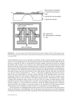
in Figures 15.8 and 15.9. Such kernels facilitate the decentralized control implementation discussed in
Section 15.4.2 and depicted in Figure 15.7,paving the way for experimental implementation with mas-
sive arrays of tiles integrating sensing, actuating, and the control logic.
The control convolution kernels shown in Figure 15.8 angle away from the wall in the upstream direction.
Coupled with the mean flow profile indicated in Figure 15.1, this accounts for the convective delay which
requires us to anticipate flow perturbations on the interior of the domain with actuation on the wall
somewhere downstream. The estimation convolution kernels shown in Figure 15.9, on the other hand,
extend well downstream of the measurement point. This accounts for the delay between the motions of
the convecting flow structures on the interior of the domain and the eventual influence of these motions
on the local drag profile on the wall; during this time delay, the flow structures responsible for these
motions convect downstream. The upstream bias of the control kernels and the downstream bias of the
estimation kernels, though physically tenable, were not prescribed in the problem formulation. A poste-
riori study of the streamwise, spanwise, and wall-normal extent, the symmetry, and the shape of such
control and estimation kernels provides us with a powerful new tool with which the fundamental physics
of this distributed fluid-mechanical system may be characterized.
The localized convolution kernels illustrated in Figures 15.8 and 15.9 are approximately independent of the
size of the computational box in which theywerecomputed, so long as this box is sufficiently large. Thus,
when implementing these kernels, we may effectively assume that they were derived in an infinite-sized box,
Model-Based Flow Control for Distributed Architectures 15-17
−0.4
−0.2
−0.6
−
0.8
−1
−0.2

−0.4
−0.8
−1.5
−0.5
0
0.5
1
0.8
0.6
0.4
0.2
0
−1
−
1
−0.6
x
y
z
−0.4
−0.6
−
0.8
−
1
−2.5
−2
−1.5
−
1

−0.5
−0.2
−0.4
0
0.5
1
0.4
0.2
0
x
z
y
−0.2
FIGURE 15.8 (Seecolor insert following page 10-34.) Localized controller gains relating the state estimate xˆ inside the
domain to the control forcing u at the point {x ϭ 0, y ϭϪ1, z ϭ 0} on the wall. Visualized are a positive and negative
isosurface of the convolution kernels for (left) the wall-normal component of velocity and (right) the wall-normal com-
ponent of vorticity. (Högberg, M., Bewley, T.R., and Henningson, D.S. (2003) “Linear Feedback Control and Estimation
of Tr ansition in Plane Channel Flow,” J. Fluid Mech. 481,pp.149–75. Reprinted with permission from Elsevier Science.)
0.5
0
−0.5
−1
−5
0
5
−4
−2
0
2
4

6
8
y
x
z
1
0.5
0
−
0.5
−5
−5
0
5
0
5
10
15
20
−1
y
x
z
1
FIGURE 15.9 (See color insert following page 10-34.) Localized estimator gains relating the measurement error
(y Ϫ y
ˆ) at the point {x ϭ 0, y ϭ Ϫ1, z ϭ 0} on the wall to the estimator forcing terms v inside the domain. Visualized
are a positive and negative isosurface of the convolution kernels for (left) the wall-normal component of velocity and
(right) the wall-normal component of vorticity. (Högberg, M., Bewley, T.R., and Henningson, D.S. (2003) “Linear
Feedback Control and Estimation of Transition in Plane Channel Flow,” J. Fluid Mech. 481, pp. 149–75. Reprinted

with permission from Elsevier Science.)
© 2006 by Taylor & Francis Group, LLC
relaxing the nonphysical assumption of spatial periodicity used in the problem formulation and modeling
the physical situation of spatially evolving flow perturbations in a spatially invariant geometry and mean flow.
The localized convolution kernels illustrated in Figures 15.8 and 15.9 are also approximately inde-
pendent of the computational mesh resolution with which theywerecomputed,when this computational
mesh is sufficiently fine. Acomputational mesh sufficient to resolve the flow under consideration also
adequately resolves these convolution kernels.
15.5.1 Open Questions
As we have shown, the framework for decentralized H
ϱ
control of the fully resolved transition problem in
the geometry depicted in Figure 15.1 is now established. Obtaining spatial localization of the convolution
kernels in physical space was the final remaining conceptual and numerical hurdle to be overcome. This
work paves the way for decentralized application of such compensation with massive arrays of identical con-
trol tiles integrating sensing, actuation, and the control logic (Figure 15.7). Though in some sense “com-
plete,” this effort has also exposed several fundamental open questions, which are now briefly discussed.
For a given choice of the matrices {B
1
, B
2
, C
1
, C
2
} and design parameters {
ᐉ
,
α
,

γ
Ͼ
γ
0
} selected, decen-
tralized H
ϱ
compensators may be determined using the procedure previously described, and performance
and robustness benchmarks may be obtained via simulation. As a final step in the control design process,
explore how much the computational effort required by the logic on each tile may be reduced without
significant degradation in the closed-loop system behavior. This can lead to a significant reduction in the
number of floating point operations per second required by the logic circuit on each tile. However, as
is discussed in Section 15.6, compensator reduction in the decentralized setting remains a significant
unsolved problem; standard reduction strategies developed for finite, closed systems are not applicable
and new research is motivated.
With the decentralized linear control framework established and prototypical numerical examples solved,
we are now in a position to explore the effectiveness of compensators computed via this framework to the
finite-amplitude perturbations that actually lead to transition and to the “large” amplitude perturbations of
fully developed turbulence, in the nonlinear equations of fluid motion. An extensive analytical and numeri-
cal study within this framework is underway. Issues regarding our preliminary efforts in this direction are
briefly reviewed in Section 15.7. As emphasized in the introduction, such a study should be guided by an
interdisciplinary perspective to be maximally successful. Specifically, such a study should fully incorporate the
known or postulated linear mechanisms leading to transition or, in the case of turbulence, the linear mecha-
nisms thought to be at least partially responsible for sustaining the turbulent cascade of energy. In addition,
this effort motivates the development of new analytical tools that might help clarify the types of state distur-
bances and flow perturbations that are particularly important in such phenomena. Armed with such an
understanding, large benefits might be realized in the compensator design because the modeling of the struc-
ture of the state disturbances exciting the system G
1
and the weighting on the flow perturbations of interest

in the cost function Q are important design criteria. In fact, we fully expect that the transfer of information
between our physical understanding of fundamental flow phenomena and our knowledge of how to control
such phenomena will be a two-way transfer. Such a strategy promises to provide powerful new tools for
obtaining fundamental physical understanding of classical problems in fluid mechanics while we gain new
insight in how to modify these phenomena by the action of control feedback.
A host of other canonical flow control problems, including the control of spatially developing bound-
ary layers, bluff-body flows, and free shear layers, should also be amenable to linear control application
using the framework outlined here. A few such extensions are discussed briefly in Section 15.8.
15.6 Compensator Reduction: Eliminating
Unnecessary Complexity
Strategies for the development of reduced-order decentralized compensators of the present form remain
a key unsolved issue. With the H
2
/H
ϱ
approach, as described previously, a physical-space state estimate in
15-18 MEMS: Introduction and Fundamentals
© 2006 by Taylor & Francis Group, LLC
the volume immediately above each tile must be updated online by the logic circuit on each tile as the
flow evolves. However, it is not necessary for the compensator to compute an accurate state estimate as
an intermediate variable; indeed, our only requirement is that, based on whatever filtered information the
dynamic compensator does extract from the noisy system measurements, suitable controls may be deter-
mined to achieve the desired closed-loop system behavior. It should be possible to reduce substantially
the complexity of the dynamic compensator and still achieve this more modest objective.
There are two possible representations in which the complexity of the compensator can be reduced: in
Fourier space (where the compensator is designed) or in physical space (where the decentralized com-
pensation is applied).
15.6.1 Fourier-Space Compensator Reduction
At any particular wavenumber pair {k
x

, k
z
}, there is one actuator variable at each wall, one sensor variable
at each wall, and a spatial discretization in y of the state variables across the domain stretching between
these walls. Because of the complete decoupling of the control problem into separate Fourier modes, the
system model used in the estimator at each particular wavenumber pair is not referenced by the com-
pensator at any other wavenumber pair. Thus, the compensators at each wavenumber pair are completely
decoupled and may be reduced independently. At certain wavenumber pairs, it might be important to
retain several degrees of freedom in the dynamic compensator, while at other wavenumber pairs, it might
be possible to retain significantly fewer degrees of freedom without significant degradation in the closed-
loop system behavior. Several existing compensator reduction strategies are well suited to this problem,
and their application in this setting is straightforward. Cortelezzi and Speyer (1998) successfully applied
the balanced truncation technique of open-loop model reduction in this Fourier-space framework to
facilitate the design of a reduced-complexity dynamic compensator.
As mentioned earlier, it is the nonorthogonality of the entire set of system eigenvectors that leads to the
peculiar (and important) possibilities for energy amplification in these systems, so compensator reduction
techniques mindful of the relevant transfer function norms are necessary. In addition, as eloquently
described by Obinata and Anderson (2000), it is most appropriate when designing low-order compen-
sators for high-order plants to reduce the compensator while accounting for how it performs in the closed
loop. An assortment of closed-loop compensator reduction techniques are now available and should be
tested in future work.
In the setting of designing a decentralized compensator, there is an important shortcoming to per-
forming standard compensator reductions in Fourier space. As the compensator reduction problem is
independent at each wavenumber pair, we might be left with a different number of degrees of freedom in
the reduced-order compensator at each wavenumber pair, leaving us with a dynamical system model that
is impossible to inverse transform back into the physical domain. Even if we restrict the compensator
reduction algorithm to reduce to the same number of degrees of freedom at each wavenumber pair (a
restrictive assumption that should be unnecessary), there appears to be no appropriate strategy currently
available to coordinate this reduction process across all wavenumbers in a consistent manner such that
the inverse transform of the reduced dynamic model is spatially localized. Without such coordination, it

seems inevitable that the ordering and representation of the various modes of this dynamic model will
be scrambled during the process of compensator reduction at each wavenumber pair, resulting in an
inverse-transform back in physical space that does not exhibit the spatial localization which is essential to
facilitate decentralized control.
15.6.2 Physical-Space Compensator Reduction
As an alternative to Fourier-space compensator reduction, one might consider instead the reduction of
the physical-space model and its associated localized convolution kernels. This has several advantages
linked to the fact that this is the actual compensation to be computed on each tile. The first advantage is
Model-Based Flow Control for Distributed Architectures 15-19
© 2006 by Taylor & Francis Group, LLC
that spatial localization will be retained, as compensator reduction is applied after the localized kernels
are obtained. Another important advantage is that this setting allows us to keep more degrees of freedom
in the dynamical system model to represent streamwise and spanwise fluctuations of the state near the
wall than we retain to represent the behavior of the state on the interior of the domain. This effectively
relaxes the restrictive assumption referred to in the previous paragraph. Such an emphasis on resolving
the state near the wall is motivated by inspection of the convolution kernels plotted in Figures 15.8 and
15.9, in which it is clear that the details of the flow near the wall are of increased importance when com-
puting the feedback.
However, the system model simulated on each individual tile is not self-contained, due to the inter-
connections with neighboring tiles indicated in Figure 15.7.Thus, if one reduces the system model above
a single tile, all neighboring tiles that reference this state estimate will be affected. As the system model is
not self-contained, as it was in the Fourier-space case, existing compensator reduction approaches are not
applicable.
An important observation, however, is that the structure of the system model carried by each tile is
identical. Due to the repeated structure of the model represented on the array, it is sufficient to optimize
the system model carried by a single tile. The repeated structure of the distributed physical-space model
should make the compensator reduction problem tractable. This fundamental problem of reducing dis-
tributed, interconnected dynamic compensators in the decentralized closed-loop setting remains, as yet,
unsolved.
15.6.3 Nonspatially Invariant Systems

Finally, it should be stated that the Fourier-space decoupling leveraged at the outset of this problem for-
mulation has been one of the key ingredients that have permitted accurate solution of well-resolved
canonical flow control problems to date. The linear control technique we have used to solve these control
problems involves the solution of matrix Riccati equations, which are accurately soluble for state dimen-
sions only up to O(10
3
). As we move to more applied flow control problems in which such Fourier-space
decoupling is either more restrictive or not available, if we continue to use Riccati-based control approaches,
creative new compensator reduction strategies will be required. We might need to apply “open-loop”
model reduction strategies (in advance of computing the control feedback and closing the loop) to make
manageable the dimension of the Riccati equations to be solved in the compensator formulation. As men-
tioned earlier, it is most appropriate when designing low-order compensators for high-order plants to
reduce the compensator while accounting for how it performs in the closed loop. Unfortunately, extremely
high-order discretizations of nonspatially invariant PDE systems will not likely afford us this luxury, as
such systems do not decouple (via Fourier transforms) into constituent lower-order control problems
amenable to matrix-based compensator design strategies.
15.7 Extrapolation: Linear Control of Nonlinear Systems
Once a decentralized linear compensator of the present form is developed, averification of its utility for
the transition problem may be obtained by applying it to the laminar flow depicted in Figure 15.1 with
either finite-amplitude (but sufficiently small) initial flow perturbations or finite-amplitude (but suffi-
ciently small) applied external disturbances. The resulting finite-amplitude flow perturbations are gov-
erned by the fully nonlinear Navier–Stokes equation and have been simulated in well resolved direct
numerical simulations (DNS) with the code benchmarked in Bewley et al. (2001). Representative simu-
lations are shown in Figure 15.10, indicating that linear compensators can indeed relaminarize perturbed
flows that would otherwise proceed rapidly towards transition to turbulence. With the framework pre-
sented here, extensive numerical studies promise to significantly extend our fundamental understanding
of the process of transition and how this process may be inhibited by control feedback.
It is also of interest to consider the application of decentralized linear compensation to the fully non-
linear problem of a turbulent flow, such as that shown in Figure 15.11. The first reason to try such an
15-20 MEMS: Introduction and Fundamentals

© 2006 by Taylor & Francis Group, LLC
Model-Based Flow Control for Distributed Architectures 15-21
10
−1
1
0
−
2
10
−
3
10
−4
0 100 200 300 400 500 600 700
Time
Energy
10
−
1
10
−
2
10
−3
0 100 200 300 400 500 600 700 800 900
Time
Energy
FIGURE 15.10 Evolution of oblique waves (left) and an initially random flow perturbation (right) added to a lam-
inar flow at Re ϭ 2000, with and without decentralized linear control feedback. The magnitude of the initial flow per-
turbations in these simulations greatly exceed the thresholds reported by Reddy et al. (1998) that lead to transition to

turbulence in an uncontrolled flow (by a factor of 225 for the oblique waves and by a factor of 15 for the random ini-
tial perturbation). Solid lines indicate the energy evolution in the controlled case, dashed lines indicate the energy
evolution in the uncontrolled case. Both of the uncontrolled systems lead quickly to transition to turbulence, whereas
both of the controlled systems relaminarize. For the controlled cases, initial perturbations with greater energy fail to
relaminarize, whereas initial perturbations with less energy relaminarize earlier. (Högberg, M., Bewley, T.R., and
Henningson, D.S. (2003) “Linear Feedback Control and Estimation of Transition in Plane Channel Flow,” J. Fluid
Mech. 481,pp.149–75. Reprinted with permission from Elsevier Science.)
FIGURE 15.11 (See color insert following page 10-34.)Visualization of the coherent structures of uncontrolled
near-wall turbulence at Re
␶
ϭ 180. Despite the geometric simplicity of this flow (see Figure 15.1), it is phenomeno-
logically rich and is characterized by a large range of length scales and time scales over which energy transport and
scalar mixing occur. The relevant spectra characterizing these complex nonlinear phenomena are continuous over this
large range of scales, thus such flows have largely eluded accurate description via dynamic models of low state dimen-
sion. The nonlinearity, the distributed nature, and the inherent complexity of its dynamics make turbulent flow sys-
tems particularly challenging for successful application of control theory. (Simulation by Bewley, T.R., Moin, P., and
Temam, R. (2001) J. Fluid Mech. Reprinted with permission of Cambridge University Press.)
© 2006 by Taylor & Francis Group, LLC
15-22 MEMS: Introduction and Fundamentals
(
a
)
ᐉ = 10
(
b
)
ᐉ = 0.5
(
c
)

ᐉ = 0.025
FIGURE 15.12 (Seecolor insert following page 10-34.) Example of the spectacular failure of linear control theory
to stabilize a simple nonlinear chaotic convection system governed by the Lorenz equation. Plotted are the regions of
attraction to the desired stationary point (blue) and to an undesired stationary point (red) in the linearly controlled
nonlinear system, and typical trajectories in each region (black and green, respectively). The cubical domain illustrated
is Ω ϭ (Ϫ25, 25)
3
in all subfigures. For clarity, different viewpoints are used in each subfigure. (Reprinted with
permission from Bewley, T.R. (1999) Phys. Fluids 11, 1169–86. Copyright 1999, American Institute of Physics.)
approach is simply because we can: linear control theory leads to implementable control algorithms and
grants a lot of flexibility in the compensator design. Nonlinear turbulence control strategies, though
currently under active development (see Sections 15.9 to 15.13), are much more difficult to design and
implement and require substantial further research before they will provide implementable control
strategies as flexible and powerful as those which we currently have at our disposal in the linear setting.
There is some evidence in the fluids literature that applying linear control feedback to turbulence
might be at least partially effective. Though the significance of this result has been debated in the fluid
mechanics community, Farrell and Ioannou (1993) have clearly shown that linearized Navier–Stokes sys-
tems in plane channel flows, when excited with the appropriate stochastic forcing, exhibit behavior rem-
iniscent of the streamwise vortices and streamwise streaks that characterize actual near-wall turbulence.
The present linear control framework (perhaps restricted to a finite horizon) should be able to exploit
whatever information the linearized Navier–Stokes equation actually contains about the mechanisms sus-
taining these turbulence structures. Though the life cycle of the near-wall coherent structures of turbu-
lence appears to involve important nonlinear phenomena [see, e.g., Hamilton et al., 1995], that in itself
does not disqualify the utility of linear control strategies to effectively disrupt critical linear terms of this
nonlinear process. Recent numerical experiments by Kim and Lim (2000) support this idea by conclu-
sively demonstrating the importance of the coupling term C in the linearized system matrix A (see
Equation (15.10)) for maintaining near-wall turbulence in nonlinear simulations.
To understand the possible pitfalls of applying linear feedback to nonlinear systems, a low-order non-
linear convection problem governed by the Lorenz equation was studied by Bewley (1999). As with the
problem of turbulent channel flow, but in a low-order system easily amenable to analysis, control feed-

back was determined with linear control theory by linearizing the governing equation about a desired
fixed point. Once a linear controller was determined by such an approach, it was then applied directly to
the fully nonlinear system. The result is depicted in Figure 15.12.
For control feedback determined by linear control theory with a large weighting
ᐉ
, on the control
effort, direct application of linear feedback to the full nonlinear system stabilizes both the desired state
and an undesired state, indicated by the two trajectories marked in Figure 15.12a. An unstable manifold
exists between these two states, indicated by the contorted surface shown. Any initial state on one side of
this manifold will converge to the desired state, and any initial state on the other side of this manifold will
converge to the undesired state.
© 2006 by Taylor & Francis Group, LLC
A
s seen in Figures 15.12b and c, as the weighting on the control effort
ᐉ
,
is turned down and the desired
stationary state is stabilized more aggressively, the domain of convergence to the undesired stabilized state
remains large. This undesired state is“aggravated” by the enhanced control feedback, moving farther from
the origin. The undesired state eventually escapes to infinity for sufficiently small
ᐉ
, indicating instability of
the nonlinear system from a wide range of initial conditions even though the desired stationary point is
endowed with a high degree of linear stability. Implication: strong linear stabilization of a desired system
state (such as laminar flow) will not necessarily eliminate undesired nonlinear system behavior (such as
turbulence) in a chaotic system.
Some form of nonlinearity in the feedback rule was required to eliminate this undesired behavior. One
effective technique is to apply a switch such that the linear control feedback is turned on only when the
state x(t) is within some sufficiently small neighborhood of the desired stabilized state x


in the linearly
controlled system. The chaotic dynamics of the uncontrolled Lorenz system will bring the system into this
neighborhood in finite time, after which control may be applied to “catch” the system at the desired equi-
librium state.
Thus, even in this simple model problem, linear feedback can have a destabilizing influence if applied
outside the neighborhood for which it was designed. For the full Navier–Stokes problem, though a certain
set of linear feedback gains might stabilize the laminar state, on the “other side of the manifold” might lie
a turbulent state aggravated by the same linear controls. Application of linear control to nonlinear chaotic
systems must therefore be done with vigilance, lest nonlinearities destabilize the closed-loop system, as
shown here. The easy fix for this low-order model problem (that is, simply turn off the control until the
chaotic dynamics bring the state into a neighborhood of the desired state) might not be available for the
(high-dimensional) problem of turbulence because fully turbulent flows appear to remain at all times far
from the laminar state.
In our preliminary attempts at applying the decentralized compensators previously developed to tur-
bulence, we have succeeded in reducing the drag of a fully developed turbulent flow by 25% with state-
feedback controllers, as shown in Figure 15.13.Interestingly, for the choice of control parameters selected
here, there is no evidence of an aggravated turbulent state. A 25% drag reduction, though significant, is
comparable to the drag reductions obtained with a variety of other ad hoc control approaches in this
flow. We are actively pursuing modification of this linear control feedback to improve upon this result.
Interdisciplinary considerations, such as those involved in the design of linear compensation for the
problem of transition, are essential in this effort. Specifically, the (unmodeled) nonlinear terms in the
Navier–Stokes equation provide insight as to the structure of the disturbances, G
1
,to be accounted for in
the linear control formulation to best compensate for their unmodeled effects. Additionally, the coherent
structures of fully developed near-wall turbulence, believed to be a major player in the self-sustaining
nonlinear process of turbulence generation near the wall, provide a phenomenological target that may be
exploited in the selection of the weighting on the flow perturbations Q in the cost function.
15.8 Generalization: Extending to Spatially Developing Flows
Extension of the decentralized linear control framework developed here to a large class of slightly nonpar-

allel flows is heuristic but straightforward. To accomplish this, the parabolic mean flow profile U(y) indi-
cated in Figure 15.1 is replaced with an appropriate “quasi-one-dimensional” profile, such as the Blasius
boundary layer profile. As long as the mean flow profile evolves slowly enough in space (as compared to
the wavelengths of the significant instabilities in the problem), it may be assumed to be constant in space
for the purpose of developing the linear control feedback. Such an assumption of slow spatial divergence
forms the foundation of the study of local and global modes used in the characterization of absolute and
convective instabilities [Huerre and Monkewitz, 1990] and has proven to be a powerful concept. For the
appropriate flows, we believe this concept is also appropriate in the context of the development of con-
trol feedback.
Implementation of the decentralized control concept in this setting is a heuristic extension of the approach
presented in Figure 15.7.Gradual variations in the mean flow are accounted for by local extension of the
Model-Based Flow Control for Distributed Architectures 15-23
© 2006 by Taylor & Francis Group, LLC
mean flow profile in the compensator derivation for each tile, gradually scaling the compensation rules
from one tile to the next as the flow develops downstream. For example, we may consider developing this
strategy for the laminar boundary layer (LBL) solutions of the Falkner–Skan–Cooke family, found by
solving the ordinary differential equation (ODE)
f ЉЈ ϩ ff Љ ϩ
β
(1 Ϫ fЈ
2
) ϭ 0
with f(0) ϭ fЈ(0) ϭ 0 and fЈ(ϱ) → 1 and defining
U ϭ U
0
fЈ(
η
) and V ϭ
Ί
๶

[
η
fЈ(
η
) Ϫ f (
η
)].
Cases of interest include the Blasius profile, modeling a zero-pressure-gradient, flat-plate LBL with
U
0
ϭ U
∞
,
β
ϭ 0,
η
ϭ y
Ί
๶
,
U
0
ᎏ
2vx
vU
0
ᎏ
2x
15-24 MEMS: Introduction and Fundamentals
FIGURE 15.13 Evolution of fully developed turbulence at RE

τ
ϭ 100 with and without decentralized linear control
feedback. This flow has approximately the same mass flux as the laminar flow at Re ϭ 2000. (Top) Energy of flow per-
turbation. (Middle) Drag (note approximately 25% reduction in the controlled cases). (Bottom) Control effort used.
The uncontrolled energy and drag are the (upper) solid lines in the top and middle figures. A gain scheduling
approach is used to tune the control feedback gains to the instantaneous mean flow profile. (Högberg, M., Bewley,
T.R., and Henningson, D.S. (2003) “Linear Feedback Control and Estimation of Transition in Plane Channel Flow,”
J. Fluid Mech. 481, pp. 149–75. Reprinted with permission from Elsevier Science.)
© 2006 by Taylor & Francis Group, LLC
the Falkner–Skan profile, modeling a nonzero-pressure-gradient LBL or wedge flow by taking
U
0
ϭ
Kx
m
,
β
ϭ
,
η
ϭ
y
Ί
๶
,
and the Falkner–Skan–Cooke profile, which models the addition of sweep to the leading edge by solving
the supplemental ODE
gЉϩ fgЈ ϭ 0
with g(0) ϭ 0 and g(ϱ) → 1 and defining W ϭ W
ϱ

g(
η
). The self-similarity of the LBL profiles might lead
to simplified parameterizations of the convolution kernels for the control and estimation problems.
Extension of this approach to a variety of other spatially developing flows (self-similar or otherwise)
should also be straightforward.
15.9 Nonlinear Optimization: Local Solutions for
Full Navier–Stokes
Given an idealized setting of full state information, no disturbances, and extensive computational
resources, significant finite-horizon optimization problems may be formulated and (locally) solved for
complex nonlinear systems using iterative, adjoint-based, gradient optimization strategies. Such opti-
mization problems can now be solved for high-dimensional discretizations of turbulent flow systems,
incorporating the full nonlinear Navier–Stokes equation, locally minimizing cost functionals represent-
ing a variety of control problems of physical interest within a given space of feasible control variables.
The mathematical framework for such optimizations will be reviewed briefly in Section 15.9.1 and is
described in greater detail by Bewley et al. (2001).
The optimizations obtained via this approach are only “local” over the domain of feasible controls
(that is, unless restrictive assumptions are made in the formulation of the control problem). Thus, the
performance obtained via this approach usually cannot be guaranteed to be “globally optimal.” However,
the performance obtained with such nonlinear optimizations often far exceeds that possible with other
control design approaches (see, e.g., Figure 15.14). In addition, this approach is quite flexible because it can
iteratively improve high-dimensional control distributions directly, as is illustrated below. Alternatively,
this approach can optimize open-loop forcing schedules, shape functions, or the coefficients of practical,
implementable, and possibly nonlinear feedback control rules. Thus, interest in adjoint-based optimiza-
tion strategies for turbulent flow systems goes far beyond that of establishing performance benchmarks
via predictive optimizations of the control distribution itself. Establishing such benchmarks is only a first
step toward a much wider range of applications for adjoint-based tools in turbulent flow systems.
The general idea of this approach, often referred to as model predictive control, is well motivated by
comparing and contrasting it to massively parallel brute-force algorithms recently developed to play the
game of chess. The goal when playing chess is to capture the other player’s king through an alternating

series of discrete moves with the opponent; at any particular turn, a player has to select one move out of
at most 20 or 30 legal alternatives.
To accomplish its optimization, a computer program designed to play the comparatively “simple”game of
chess, such as Deep Blue [Newborn, 1997], must, in the worst case, plan ahead by iteratively examining a
tree of possible evolutions of the game several moves into the future [Atkinson, 1993], a strategy based
on “function evaluations” alone. At each step, the program selects the move that leads to its best expected
outcome, given that the opponent is doing the same in a truly noncooperative competition. The version
of Deep Blue that defeated Garry Kasparov in 1997 was able to calculate up to 200 billion moves in the
three minutes it was allowed to conduct each turn. Even with this extreme number of function evalua-
tions at its disposal on this relatively simple problem, the algorithm was only about an even match with
Kasparov’s human intuition.
(m ϩ 1)U
0
ᎏᎏ
2vx
2m
ᎏ
1 ϩ m
Model-Based Flow Control for Distributed Architectures 15-25
© 2006 by Taylor & Francis Group, LLC