Steel Designer''''s Manual Part 5 pptx
Bạn đang xem bản rút gọn của tài liệu. Xem và tải ngay bản đầy đủ của tài liệu tại đây (1.04 MB, 80 trang )
Element analysis 287
9.1.1 Equations of static equilibrium
From Newton’s law of motion, the conditions under which a body remains in static
equilibrium can be expressed as follows:
•
The sum of the components of all forces acting on the body, resolved along any
arbitrary direction, is equal to zero. This condition is completely satisfied if the
components of all forces resolved along the x, y, z directions individually add up
to zero. (This can be represented by SP
x
= 0, SP
y
= 0, SP
z
= 0, where P
x
, P
y
and
P
z
represent forces resolved in the x, y, z directions.) These three equations
represent the condition of zero translation.
•
The sum of the moments of all forces resolved in any arbitrarily chosen plane
about any point in that plane is zero. This condition is completely satisfied when
all the moments resolved into xy, yz and zx planes all individually add up to zero.
(SM
xy
= 0, SM
yz
= 0 and SM
zx
= 0.) These three equations provide for zero
rotation about the three axes.
If a structure is planar and is subjected to a system of coplanar forces, the
conditions of equilibrium can be simplified to three equations as detailed below:
•
The components of all forces resolved along the x and y directions will individ-
ually add up to zero (SP
x
= 0 and SP
y
= 0).
•
The sum of the moments of all the forces about any arbitrarily chosen point in
the plane is zero (i.e. SM = 0).
9.1.2 The principle of superposition
This principle is only applicable when the displacements are linear functions of
applied loads. For structures subjected to multiple loading, the total effect of several
loads can be computed as the sum of the individual effects calculated by applying
the loads separately. This principle is a very useful tool in computing the combined
effects of many load effects (e.g. moment, deflection, etc.). These can be calculated
separately for each load and then summed.
9.2 Element analysis
Any complex structure can be looked upon as being built up of simpler units or
components termed ‘members’ or ‘elements’. Broadly speaking, these can be
classified into three categories:
•
Skeletal structures consisting of members whose one dimension (say, length) is
much larger than the other two (viz. breadth and height). Such a line element is
Steel Designers' Manual - 6th Edition (2003)
This material is copyright - all rights reserved. Reproduced under licence from The Steel Construction Institute on 12/2/2007
To buy a hardcopy version of this document call 01344 872775 or go to
288 Introduction to manual and computer analysis
variously termed as a bar, beam, column or tie. A variety of structures are
obtained by connecting such members together using rigid or hinged joints.
Should all the axes of the members be situated in one plane, the structures so
produced are termed plane structures. Where all members are not in one plane,
the structures are termed space structures.
•
Structures consisting of members whose two dimensions (viz. length and breadth)
are of the same order but much greater than the thickness fall into the second
category. Such structural elements are called plated structures. Such structural
elements are further classified as plates and shells depending upon whether they
are plane or curved. In practice these units are used in combination with beams
or bars. Slabs supported on beams, cellular structures, cylindrical or spherical
shells are all examples of plated structures.
•
The third category consists of structures composed of members having all the
three dimensions (viz. length, breadth and depth) of the same order. The
analysis of such structures is extremely complex, even when several simplifying
assumptions are made. Dams, massive raft foundations, thick hollow spheres,
caissons are all examples of three-dimensional structures.
For the most part the structural engineer is concerned with skeletal structures.
Increasing sophistication in available techniques of analysis has enabled the eco-
nomic design of plated structures in recent years. Three-dimensional analysis of
structures is only rarely carried out. Under incremental loading, the initial defor-
mation or displacement response of a steel member is elastic. Once the stresses
caused by the application of load exceed the yield point, the cross section gradually
yields. The gradual spread of plasticity results initially in an elasto-plastic response
and then in plastic response, before ultimate collapse occurs.
9.3 Line elements
The deformation response of a line element is dependent on a number of cross-
sectional properties such as area, A, second moment of area (I
xx
=Úy
2
dA;
I
yy
=Úx
2
dA) and the product moment of area (I
xy
=ÚxydA). The two axes xx and yy
are orthogonal. For doubly symmetric sections, the axes of symmetry are those for
which Úxy dA = 0. These are known as principal axes. For a plane area, the principal
axes may be defined as a pair of rectangular axes in its plane and passing through
its centroid, such that the product moment of area ÚxydA = 0, the co-ordinates
referring to the principal axes. If the plane area has an axis of symmetry, it is
obviously a principal axis (by symmetry Úxy dA = 0). The other axis is at right angles
to it, through the centroid of the area.
Tables of properties of the section (including the centroid and shear centre of
the section) are available as published data (e.g. SCI Steelwork Design Guide,
Vol. 1).
1
Steel Designers' Manual - 6th Edition (2003)
This material is copyright - all rights reserved. Reproduced under licence from The Steel Construction Institute on 12/2/2007
To buy a hardcopy version of this document call 01344 872775 or go to
V
y
U
x
Line elements 289
If the section has no axis of symmetry (e.g. an angle section) the principal axes
will have to be determined. Referring to Fig. 9.1, if uOu and vOv are the principal
axes, the angle a between the uu and xx axes is given by
(9.1)
(9.2)
The values of a, I
uu
and I
vv
are available in published steel design guides (e.g.
Reference 1).
9.3.1 Elastic analysis of line elements under axial loading
When a cross section is subjected to a compressive or tensile axial load,P, the result-
ing stress is given by the load/area of the section, i.e. P/A. Axial load is defined as
one acting at the centroid of the section. When loads are introduced into a section
in a uniform manner (e.g. through a heavy end-plate), this represents the state of
stress throughout the section. On the other hand, when a tensile load is introduced
via a bolted connection, there will be regions of the member where stress concen-
trations occur and plastic behaviour may be evident locally, even though the mean
stress across the section is well below yield.
If the force P is not applied at the centroid, the longitudinal direct stress distri-
bution will no longer be uniform. If the force is offset by eccentricities of e
x
and e
y
measured from the centroidal axes in the y and x directions, the equivalent set of
actions are (1) an axial force P, (2) a bending moment M
x
= Pe
x
in the yz plane and
(3) a bending moment M
y
= Pe
y
in the zx plane (see Fig. 9.2). The method of eval-
uating the stress distribution due to an applied moment is given in a later section.
I
II II
I
vv
xx yy xx yy
xy
=
+
-
-
+
22
22cos sinaa
I
II II
I
uu
xx yy xx yy
xy
=
+
+
-
-
22
22cos sinaa
tan 2
2
a =
-
-
I
II
xy
xx yy
Fig. 9.1 Angle section (no axis of symmetry)
Steel Designers' Manual - 6th Edition (2003)
This material is copyright - all rights reserved. Reproduced under licence from The Steel Construction Institute on 12/2/2007
To buy a hardcopy version of this document call 01344 872775 or go to
y
ey
y
290 Introduction to manual and computer analysis
The total stress at any section can be obtained as the algebraic sum of the stresses
due to P, M
x
and M
y
.
9.3.2 Elastic analysis of line elements in pure bending
For a section having at least one axis of symmetry and acted upon by a bending
moment in the plane of symmetry, the Bernoulli equation of bending may be used
as the basis to determine both stresses and deflections within the elastic range. The
assumptions which form the basis of the theory are:
•
The beam is subjected to a pure moment (i.e. shear is absent). (Generally the
deflections due to shear are small compared with those due to flexure; this is not
true of deep beams.)
•
Plane sections before bending remain plane after bending.
•
The material has a constant value of modulus of elasticity (E) and is linearly
elastic.
The following equation results (see Fig. 9.3).
(9.3)
where M is the applied moment; I is the second moment of area about the neutral
axis; f is the longitudinal direct stress at any point within the cross section; y is the
distance of the point from the neutral axis; E is the modulus of elasticity; R is the
radius of curvature of the beam at the neutral axis.
M
I
f
y
E
R
==
Fig. 9.2 Compressive force applied eccentrically with reference to the centroidal axis
Steel Designers' Manual - 6th Edition (2003)
This material is copyright - all rights reserved. Reproduced under licence from The Steel Construction Institute on 12/2/2007
To buy a hardcopy version of this document call 01344 872775 or go to
-*
cross section
stress diagram
neutral axis
Line elements 291
From the above, the stress at any section can be obtained as
For a given section (having a known value of I) the stress varies linearly from zero
at the neutral axis to a maximum at extreme fibres on either side of the neutral axis:
(9.4)
The term Z is known as the elastic section modulus and is tabulated in section tables.
1
The elastic moment capacity of a given section may be found directly as the product
of the elastic section modulus, Z, and the maximum allowable stress.
If the section is doubly symmetric, then the neutral axis is mid-way between the
two extreme fibres. Hence, the maximum tensile and compressive stresses will be
equal. For an unsymmetric section this will not be the case, as the value of y for the
two extreme fibres will be different.
For a monosymmetric section, such as the T-section shown in Fig. 9.4, subjected
to a moment acting in the plane of symmetry, the elastic neutral axis will be the
centroidal axis. The above equations are still valid. The values of y
max
for the two
extreme fibres (one in compression and the other in tension) are different. For an
applied sagging (positive) moment shown in Fig. 9.4, the extreme fibre stress in the
flange will be compressive and that in the stalk will be tensile.The numerical values
of the maximum tensile and compressive stresses will differ. In the case sketched in
Fig.9.4,the magnitude of the tensile stress will be greater, as y
max
in tension is greater
than that in compression.
Caution has to be exercised in extending the pure bending theory to asymmetric
sections. There are two special cases where no twisting occurs:
f
My
I
M
Z
Z
I
y
max
max
max
.
==
=where
f
My
I
=
Fig. 9.3 Pure bending
Steel Designers' Manual - 6th Edition (2003)
This material is copyright - all rights reserved. Reproduced under licence from The Steel Construction Institute on 12/2/2007
To buy a hardcopy version of this document call 01344 872775 or go to
y
292 Introduction to manual and computer analysis
•
Bending about a principal axis in which no displacement perpendicular to the
plane of the applied moment results.
•
The plane of the applied moment passes through the shear centre of the cross
section.
When a cross section is subjected to an axial load and a moment such that no
twisting occurs, the stresses may be determined by resolving the moment into com-
ponents M
uu
and M
vv
about the principal axes uu and vv and combining the result-
ing longitudinal stresses with those resulting from axial loading:
(9.5)
For a section having two axes of symmetry (see Fig. 9.2) this simplifies to
Pure bending does not cause the section to twist. When the shear force is applied
eccentrically in relation to the shear centre of the cross section, the section twists
and initially plane sections no longer remain plane. The response is complex and
consists of a twist and a deflection with components in and perpendicular to the
plane of the applied moment. This is not discussed in this chapter. A simplified
method of calculating the elastic response of cross sections subjected to twisting
moments is given in an SCI publication.
2
9.3.3 Elastic analysis of line elements subject to shear
Pure bending discussed in the preceding section implies that the shear force applied
on the section is zero. Application of transverse loads on a line element will, in
general, cause a bending moment which varies along its length, and hence a shear
force which also varies along the length is generated.
f
P
A
My
I
Mx
I
xy
xx
xx
yy
yy
,
=± ± ±
f
P
A
Mv
I
Mu
I
uv
uu
uu
vv
vv
,
=± ± ±
Fig. 9.4 Monosymmetric section subjected to bending
Steel Designers' Manual - 6th Edition (2003)
This material is copyright - all rights reserved. Reproduced under licence from The Steel Construction Institute on 12/2/2007
To buy a hardcopy version of this document call 01344 872775 or go to
b
shear stress
distribution
rectangular
cross section
(a)
T
qmax)
I
-I shear stress
distribution
I—section
(b)
Line elements 293
If the member remains elastic and is subjected to bending in a plane of
symmetry (such as the vertical plane in a doubly symmetric or monosymmetric
beam), then the shear stresses caused vary with the distance from the neutral
axis.
For a narrow rectangular cross section of breadth b and depth d, subjected to a
shear force V and bent in its strong direction (see Fig. 9.5(a)), the shear stress varies
parabolically from zero at the lower and upper surfaces to a maximum value, q
max
,
at the neutral axis given by
i.e. 50% higher than the average value.
For an I-section (Fig. 9.5(b)), the shear distribution can be evaluated from
(9.6)
where B is the breadth of the section at which shear stress is evaluated. The
integration is performed over that part of the section remote from the neutral axis,
i.e. from y = h to y = h
max
with a general variable width of b.
Clearly, for the I- (or T-) section, at the web/flange interface the value of the
integral will remain constant.As the section just inside the web becomes the section
just inside the flange, the value of the vertical shear abruptly changes as B changes
from web thickness to flange width.
q
V
IB
by y
yh
yh
=
=
=
Ú
d
max
q
V
bd
max
=
3
2
Fig. 9.5 Shear stress distribution: (a) in a rectangular cross section and (b) in an I-section
Steel Designers' Manual - 6th Edition (2003)
This material is copyright - all rights reserved. Reproduced under licence from The Steel Construction Institute on 12/2/2007
To buy a hardcopy version of this document call 01344 872775 or go to
yield point
/
0
strain hardening
<
strain hardening commences
strain
294 Introduction to manual and computer analysis
9.3.4 Elements stressed beyond the elastic limit
The most important characteristic of structural steels (possessed by no other
material to the same degree), is their capacity to withstand considerable deforma-
tion without fracture. A large part of this deformation occurs during the process of
yielding, when the steel extends at a constant and uniform stress known as the yield
stress.
Figure 9.6 shows, in its idealized form, the stress–strain curve for structural steels
subjected to direct tension. The line 0A represents the elastic straining of the
material in accordance with Hooke’s law. From A to B, the material yields while the
stress remains constant and is equal to the yield stress, f
y
. The strain occurring in
the material during yielding remains after the load has been removed and is called
plastic strain. It is important to note that this plastic strain AB is at least ten times
as large as the elastic strain, e
y
, at yield point.
When subjected to compression, various grades of structural steel behave in a
similar manner and display the same property of yield. This characteristic is known
as ductility of steel.
9.3.5 Bending of beams beyond the elastic limit
For simplicity, the case of a beam symmetrical about both axes is considered first.
The fibres of the beam subjected to bending are stressed in tension or compression
according to their position relative to the neutral axis and are strained as shown in
Fig. 9.7.
While the beam remains entirely elastic, the stress in every fibre is proportional
to its strain and to its distance from the neutral axis. The stress, f, in the extreme
fibres cannot exceed the yield stress, f
y
.
When the beam is subjected to a moment slightly greater than that which first
produces yield in the extreme fibres, it does not fail. Instead, the outer fibres yield
Fig. 9.6 Idealized stress–strain relationship for mild steel
Steel Designers' Manual - 6th Edition (2003)
This material is copyright - all rights reserved. Reproduced under licence from The Steel Construction Institute on 12/2/2007
To buy a hardcopy version of this document call 01344 872775 or go to
(a)
(b) (c) (d)
plastic zones
/ (comp.) \
H
plastic zones
Y
strain distribution
(tension)
(a)
(b)
(c) (d)
Line elements 295
at constant stress, f
y
, while the fibres nearer to the neutral axis sustain increased
elastic stresses. Figure 9.8 shows the stress distribution for beams subjected to
such moments. Such beams are said to be partially plastic and those portions of their
cross sections which have reached the yield stress are described as plastic zones.
The depths of the plastic zones depend upon the magnitude of the applied
moment. As the moment is increased, the plastic zones increase in depth, and it is
assumed that plastic yielding will continue to occur at yield stress, f
y
, resulting in
two stress blocks, one zone yielding in tension and one in compression. Figure 9.9
represents the stress distribution in beams stressed to this stage. The plastic zones
occupy the whole area of the sections,which are then described as being fully plastic.
When the cross section of a member is fully plastic under a bending moment, any
attempt to increase this moment will cause the member to act as if hinged at that
point. This point is then described as a plastic hinge.
Fig. 9.7 Elastic distribution of stress and strain in a symmetric beam. (a) Rectangular
section, (b) I-section, (c) stress distribution for (a) or (b), (d) strain distribution for
(a) or (b)
Fig. 9.8 Distribution of stress and strain beyond the elastic limit for a symmetric beam.
(a) Rectangular section, (b) I-section, (c) stress distribution for (a) or (b), (d) strain
distribution for (a) or (b)
Steel Designers' Manual - 6th Edition (2003)
This material is copyright - all rights reserved. Reproduced under licence from The Steel Construction Institute on 12/2/2007
To buy a hardcopy version of this document call 01344 872775 or go to
___ __
PH
dEl nerfis
_
fy 4
(a) (b) (c)
(d)
296 Introduction to manual and computer analysis
The bending moment producing a plastic hinge is called the fully plastic moment
and is denoted by M
p
. As the total compressive force and the total tensile force on
the cross section must be equal, it follows that the plastic neutral axis is also the
equal area axis, i.e. half the area of section is plastic in tension and the other half is
plastic in compression. This is true for monosymmetric or unsymmetrical sections
as well.
Shape factor
As described previously there will be two stress blocks, one in tension, the other in
compression, each at yield stress. For equilibrium of the cross section, the areas in
compression and tension must be equal. For a rectangular section the plastic
moment can be calculated as
which is 1.5 times the elastic moment capacity.
It will be noted that, in developing this increased moment, there is large strain-
ing in the external fibres of the section together with large rotations and deflections.
The behaviour may be plotted as a moment–rotation curve. Curves for various
sections are shown in Fig. 9.10.
The ratio of the plastic modulus, S, to the elastic modulus, Z, is known as the
shape factor, , and it will govern the point in the moment–rotation curve when
non-linearity starts. For the ideal section in bending, i.e. two flange plates, this
will have a value of unity. The value increases for more material at the centre of
the section. For a universal beam, the value is about 1.15 increasing to 1.5 for a
rectangle.
Mb
dd
f
bd
f
pyy
==2
24 4
2
Fig. 9.9 Distribution of stress and strain in a fully plastic cross section. (a) Rectangular
section, (b) I-section, (c) stress distribution for (a) or (b), (d) strain distribution for
(a) or (b)
Steel Designers' Manual - 6th Edition (2003)
This material is copyright - all rights reserved. Reproduced under licence from The Steel Construction Institute on 12/2/2007
To buy a hardcopy version of this document call 01344 872775 or go to
(i'1.15)
(u=1.50)
(v1 .00)
1.00
0.87
0.67
M= jyMp
curvature
Line elements 297
Plastic hinges and rigid plastic analysis
In deciding the manner in which a beam may fail it is desirable to understand the
concept of how plastic hinges form when the beam becomes fully plastic. The
number of hinges necessary for failure does not vary for a particular structure
subject to a given loading condition, although a part of a structure may fail
independently by the formation of a smaller number of hinges. The member or
structure behaves in the manner of a hinged mechanism, and, in doing so, adjacent
hinges rotate in opposite directions.
As the plastic deformations at collapse are considerably larger than elastic ones,
it is assumed that the line element remains rigid between supports and hinge
positions i.e. all plastic rotation occurs at the plastic hinges.
Considering a simply-supported beam subjected to a point load at mid-span
(Fig. 9.11), the maximum strain will take place at the centre of the span where a
plastic hinge will be formed at yield of full section. The remainder of the beam will
remain straight: thus the entire energy will be absorbed by the rotation of the plastic
hinge.
Work done at the plastic hinge = M
p
(2q)
Work done by the displacement of the load =
At collapse, these two must be equal:
The moment at collapse of an encastré beam with a uniformly distributed load
(w = W/L) is worked out in a manner similar to the above from Fig. 9.12.
2
2
44
M
WL
WML MWL
p
pp
or
qq=
==
W
L
2
q
Ê
Ë
ˆ
¯
Fig. 9.10 Moment–rotation curves
Steel Designers' Manual - 6th Edition (2003)
This material is copyright - all rights reserved. Reproduced under licence from The Steel Construction Institute on 12/2/2007
To buy a hardcopy version of this document call 01344 872775 or go to
I__
L
1!
I
I
I
I
lii
plastic
w
zone
I
yield zone
stiff length
B
M
bending moment diagram
B
moment—rotation curve
M
w/unit length
/
A
I II I I
I I I
)M8
loading
(A
C
L
I
-i
collapse
Mp
B
M.
298 Introduction to manual and computer analysis
Work done at the three plastic hinges = M
p
(q + 2q + q) = 4M
p
q
Work done by the displacement of the load
Equating the two,
The moments at collapse for other conditions of loading can be worked out by a
similar procedure.
WML
MWL
=
=
16
16
p
p
or
WL
M
4
4qq=
p
W
W
L
LL WL
()
==
22 4
Fig. 9.11 Centrally-loaded simply-supported beam
Fig. 9.12 Encastré beam with a uniformly distributed load
Steel Designers' Manual - 6th Edition (2003)
This material is copyright - all rights reserved. Reproduced under licence from The Steel Construction Institute on 12/2/2007
To buy a hardcopy version of this document call 01344 872775 or go to
Line elements 299
9.3.6 Load factor and theorems of plastic collapse
The load factor at rigid plastic collapse, l
p
, is defined as the lowest multiple of the
design loads which will cause the whole structure, or any part of it, to become a
mechanism.
In the limit-state approach, the designer seeks to ensure that at the appropriate
factored loads the structure will not fail. Thus the rigid plastic load factor, l
p
, must
not be less than unity, under factored loads.
The number of independent mechanisms, n, is related to the number of possible
plastic hinge locations, h, and the degree of redundancy, r, of the skeletal structure,
by the equation
n = h - r
The three theorems of plastic collapse are given below for reference:
(1) Lower bound or static theorem
A load factor, l
s
, computed on the basis of an arbitrarily assumed bending
moment diagram which is in equilibrium with the applied loads and where the
fully plastic moment of resistance is nowhere exceeded, will always be less than,
or at best equal to, the load factor at rigid plastic collapse, l
p
.
l
p
is the highest value of l
s
which can be found.
(2) Upper bound or kinematic theorem
A load factor, l
k
, computed on the basis of an arbitrarily assumed mechanism
will always be greater than, or at best equal to, the load factor at rigid plastic
collapse, l
p
.
l
p
is the lowest value of l
k
which can be found.
(3) Uniqueness theorem
If both the above criteria ((1) and (2)) are satisfied, then l = l
p
.
9.3.7 Effect of axial load and shear
If a member is subjected to the combined action of bending moment and axial force,
the plastic moment capacity will be reduced.
The presence of an axial load implies that the sum of the tension and compres-
sion forces in the section is not zero (see Fig. 9.13).This means that the neutral axis
moves away from the equal area axis, providing an additional area in tension or
compression depending on the type of axial load. The presence of shear forces will
also reduce the moment capacity. For the beam sketched in Fig. 9.13,
axial load resisted = 2atf
y
Defining
axial force resisted
axial capacity of section
n
at
A
==
2
,
Steel Designers' Manual - 6th Edition (2003)
This material is copyright - all rights reserved. Reproduced under licence from The Steel Construction Institute on 12/2/2007
To buy a hardcopy version of this document call 01344 872775 or go to
T
B
f
total area = A
total stresses = bending + axial compression
300 Introduction to manual and computer analysis
For a given cross section, the plastic moment capacity, M
p
, can be evaluated as
explained previously.The reduced moment capacity, M¢
p
, in the presence of the axial
load can be calculated as follows:
(9.7)
where S is the plastic modulus of the section.
Section tables provide the moment capacity for available steel sections using the
approach given above.
1
Similar expressions will be obtained for minor axis bending.
9.3.8 Plastic analysis of beams subjected to shear
Once the material in a beam has started to yield in a longitudinal direction, it is
unable to sustain applied shear. When a shear, V, and an applied moment, M, are
applied simultaneously to an I-section, a simplifying assumption is employed to
reduce the complexity of calculations; shear resistance is assumed to be provided
by the web, hence the shear stress in the web is obtained as a constant value of V
divided by the web area (see Fig. 9.14).The longitudinal direct stress to cause yield,
f
1
, in the presence of this shear stress, q, is obtained by using the von Mises yield
criterion:
3
f
2
y
= f
2
1
+ 3q
2
The reduced plastic moment capacity is given by
(9.8)
MM
ff
f
M
rp
y1
y
pw
=-
-
Ê
Ë
Á
ˆ
¯
˜
MMtaf
Mt
nA
t
fS
nA
t
f
pp y
py y
¢
=-
=- =-
Ê
Ë
Á
ˆ
¯
˜
2
22
2
22
4
4
a
nA
t
=
2
Fig. 9.13 The effect of combined bending and compression
Steel Designers' Manual - 6th Edition (2003)
This material is copyright - all rights reserved. Reproduced under licence from The Steel Construction Institute on 12/2/2007
To buy a hardcopy version of this document call 01344 872775 or go to
jd
f
shear stress
longitudinal stress
(a) (b) (c)
Line elements 301
where M
pw
is the fully plastic moment of resistance of the web.
The addition of an axial load to the above condition can be dealt with by
shifting the neutral axis, as was done in Fig. 9.13.The web area required to carry the
axial load is now given by P/f
1
and the depth of the web, d
a
, corresponding to this
is given by
A further reduction in moment due to the introduction of the axial load is given
by
Hence the reduced moment capacity of the section is given by
(9.9)
where
9.3.9 Plastic analysis for more than one condition of loading
When more than one condition of loading is to be applied to a line element, it may
not always be obvious which is critical. It is necessary then to perform separate
calculations, one for each loading condition, the section being determined by the
solution requiring the largest plastic moment.
f
fq
1y
=-
()
22
3.
MM
ff
f
M
td
f
1p
y1
y
pw
wa
1
=-
-
Ê
Ë
Á
ˆ
¯
˜
-
2
4
td
f
wa
2
1
4
d
P
ft
a
1w
=
Fig. 9.14 Combined bending and shear
Steel Designers' Manual - 6th Edition (2003)
This material is copyright - all rights reserved. Reproduced under licence from The Steel Construction Institute on 12/2/2007
To buy a hardcopy version of this document call 01344 872775 or go to
cTy
302 Introduction to manual and computer analysis
Unlike the elastic method of design in which moments produced by different
loading systems can be added together, the opposite is true for the plastic theory.
Plastic moments obtained by different loading systems cannot be combined, i.e.
the plastic moment calculated for a given set of loads is only valid for that loading
condition.This is because the principle of superposition becomes invalid when parts
of the structure have yielded.
9.4 Plates
Most steel structures consist of members which can be idealized as line elements.
However, structural components having significant dimensions in two directions
(viz. plates) are also encountered frequently.In steel structures,plates occur as com-
ponents of I-, H-, T- or channel sections as well as in structural hollow sections.
Sheets used to enclose lift shafts or walls or cladding in framed structures are also
examples of plates.
With plane sheets, the stiffness and strength in all directions is identical and the
plate is termed isotropic. This is no longer true when stiffeners or corrugations are
introduced in one direction.The stiffnesses of the plate in the x and y directions are
substantially different. Such a plate is termed orthotropic.
The x and y axes for the analysis of the plate are usually taken in the plane of the
plate, as shown in Fig. 9.15, while the z axis is perpendicular to that plane. An
element of the plate will be subjected to six stress components: three direct stresses
(s
x
, s
y
and s
z
) and three shear stresses (t
xy
, t
yz
and t
zx
). There are six corresponding
strains: three direct strains (e
x
, e
y
and e
z
) and three shear strains (g
xy
, g
yz
and g
zx
).
These stresses and strains are related in the elastic region by the material proper-
ties Young’s modulus (E) and Poisson’s ratio (v).
When considering the response of the plate, the approach customarily employed
is termed plane stress idealization.As the thickness, t, of the plate is small compared
with its other two dimensions in the x and y directions, the stresses having compon-
ents in the z direction are negligible (i.e. s
z
, t
yz
and t
xz
are all zero).This implies that
Fig. 9.15 Stress components on an element
Steel Designers' Manual - 6th Edition (2003)
This material is copyright - all rights reserved. Reproduced under licence from The Steel Construction Institute on 12/2/2007
To buy a hardcopy version of this document call 01344 872775 or go to
Analysis of skeletal structures 303
the out-of-plane displacement is not zero, and this condition is referred to as plane
stress idealization.
For an isotropic plate, the general equation relating the displacement, w,
perpendicular to the plane of the plate element is given by
(9.10)
where q is the normal applied load per unit area in the z direction which will, in
general, vary with x and y. The term D is the flexural rigidity of the plate, given by
(9.11)
The main difficulty in using this approach lies in the choice of a suitable
displacement function, w, which satisfies the boundary conditions. For loading
conditions other than the simplest, an exact solution of this differential equation is
virtually impossible. Hence approximate methods (e.g. multiple Fourier series) are
utilized. Once a satisfactory displacement function, w, is obtained, the moments per
unit width of the plate may be derived from
(9.12)
For orthotropic plates, the stiffness in x and y directions is different and the
equations are suitably modified as given below:
(9.13)
where D
x
and D
y
are the flexural rigidities in the two directions.
In view of the difficulty of using classical methods for the solution of plate
problems, finite element methods have been developed in recent years to provide
satisfactory answers.
9.5 Analysis of skeletal structures
The evaluation of the stress resultants in members of skeletal frames involves the
solution of a number of simultaneous equations.When a structure is in equilibrium,
every element or constituent part of it is also in equilibrium. This property is made
use of in developing the concept of the free body diagram for elements of a structure.
D
w
x
D
w
x
y
D
w
y
q
xxy y
∂
∂
+
∂
∂∂
+
∂
∂
=
4
4
4
22
4
4
2
MD
w
x
w
y
MD
w
y
w
x
MMD
w
xy
x
y
xy yx
=-
∂
∂
+
∂
∂
Ê
Ë
Á
ˆ
¯
˜
=-
∂
∂
+
∂
∂
Ê
Ë
Á
ˆ
¯
˜
=- = -
()
∂
∂∂
2
2
2
2
2
2
2
2
2
1
D
Et
=
-
()
3
2
12 1
∂
∂
+
∂
∂∂
+
∂
∂
=
4
4
4
22
4
4
2
w
x
w
x
y
w
y
q
D
Steel Designers' Manual - 6th Edition (2003)
This material is copyright - all rights reserved. Reproduced under licence from The Steel Construction Institute on 12/2/2007
To buy a hardcopy version of this document call 01344 872775 or go to
(0)
(b)
304 Introduction to manual and computer analysis
The portal frame sketched in Fig. 9.16 will now be considered for illustrating the
concept. Assuming that there is an imaginary cut at E on the beam BC, the part
ABE continues to be in equilibrium if the two forces and moment which existed at
section E of the uncut frame are applied externally.The internal forces which existed
at E are given by (1) an axial force F, (2) a shear force V and (3) a bending moment
M. These are known as stress resultants. The external forces on ABE, together with
the forces F, V and M, keep the part ABE in equilibrium; Fig. 9.16(b) is called the
free body diagram. On a rigid jointed plane frame there are three stress resultants
at each imaginary cut. The part ECD must also remain in equilibrium. This
consideration leads to a similar set of forces F, V and M shown in Fig. 9.16(c). It
will be noted that the forces acting on the cut face E are equal and opposite. If the
two free body diagrams are moved towards each other, it is obvious the internal
forces F, V and M cancel out and the structure is restored to its original state of
equilibrium. As previously stated, equilibrium implies SP
x
= 0; SP
y
= 0; SM = 0 for
a planar structure. These equations can be validly applied by considering the struc-
ture as a whole, or by considering the free body diagram of a part of a structure.
In a similar manner, it can be seen that a three-dimensional rigid-jointed
frame has six stress resultants across each section. These are the axial force, two
shears in two mutually perpendicular directions and three moments, as shown in
Fig. 9.17.
Fig. 9.16 Free body diagram
Fig. 9.17 Force and moments in x, y and z directions
Steel Designers' Manual - 6th Edition (2003)
This material is copyright - all rights reserved. Reproduced under licence from The Steel Construction Institute on 12/2/2007
To buy a hardcopy version of this document call 01344 872775 or go to
P
flexibility of
___________________
spring = 4-
flexibility of beam = 4-
(0)
(b)
Analysis of skeletal structures 305
With pin-jointed frames, be they two- or three-dimensional, there is only one
stress resultant per member, viz. its axial load. When forces act on an elastic struc-
ture, it undergoes deformations, causing displacements at every point within the
structure.
The solution of forces in the frames is accomplished by relating the stress result-
ants to the displacements. The number of equations needed is governed by the
degrees of freedom, i.e. the number of possible component displacements. At one
end of the member of a pin-jointed plane frame, the member displacement has
translational components in the x and y directions only, and no rotational displace-
ment. The number of degrees of freedom is two. By similar reasoning it will be
apparent that the number of degrees of freedom for a rigid-jointed plane frame
member is three. For a member of a three-dimensional pin-jointed frame it is also
three, and for a similar rigid-jointed frame it is six.
9.5.1 Stiffness and flexibility
Forces and displacements have a vital and interrelated role in the analysis of struc-
tures. Forces cause displacements and the occurrence of displacements implies the
existence of forces.The relationship between forces and displacements is defined in
one of two ways, viz. flexibility and stiffness.
Flexibility gives a measure of displacements associated with a given set of forces
acting on the structure. This concept will be illustrated by considering the example
of a spring loaded at one end by a static load P (see Fig. 9.18).
As the spring is linearly elastic, the extension, D, produced is directly propor-
tional to the applied load, P. The deflection produced by a unit load (defined as the
flexibility of the spring) is obviously D/P. Figure 9.18(b) illustrates the deflection
response of a beam to an applied load P. Once again the flexibility of the beam is
D/P.
In the simple cases considered above, flexibility simply gives the load–displace-
ment response at a point. A more generalized definition applicable to the displace-
Fig. 9.18 Flexibility
Steel Designers' Manual - 6th Edition (2003)
This material is copyright - all rights reserved. Reproduced under licence from The Steel Construction Institute on 12/2/2007
To buy a hardcopy version of this document call 01344 872775 or go to
306 Introduction to manual and computer analysis
ment response at a number of locations will now be obtained by considering the
beam sketched in Fig. 9.19.
Considering a unit load acting at point 1 (Fig. 9.19(b)), the corresponding deflec-
tions at points 1, 2 and 3 are denoted as f
11
, f
21
and f
31
(the first subscript denotes
the point at which the deflection is measured; the second subscript refers to the
point at which the unit load is applied).The terms f
11
, f
21
, f
31
are called flexibility coef-
ficients. Figure 9.19(c) and (d) give the corresponding flexibility coefficients for load
positions 2 and 3 respectively. By the principle of superposition, the total deflections
at points 1, 2 and 3 due to P
1
,P
2
and P
3
can be written as
D
1
= P
1
f
11
+ P
2
f
12
+ P
3
f
13
D
2
= P
1
f
21
+ P
2
f
22
+ P
3
f
23
D
3
= P
1
f
31
+ P
2
f
32
+ P
3
f
33
Written in matrix form, this becomes
(9.14)
D
D
D
1
2
3
11 12 13
21 22 23
31 32 33
1
2
3
Ï
Ì
Ô
Ó
Ô
¸
˝
Ô
˛
Ô
=
È
Î
Í
Í
Í
˘
˚
˙
˙
˙
Ï
Ì
Ô
Ó
Ô
¸
˝
Ô
˛
Ô
fff
fff
fff
P
P
P
Fig. 9.19 Flexibility coefficients for a loaded beam
Steel Designers' Manual - 6th Edition (2003)
This material is copyright - all rights reserved. Reproduced under licence from The Steel Construction Institute on 12/2/2007
To buy a hardcopy version of this document call 01344 872775 or go to
k
Analysis of skeletal structures 307
or {D}= [F]{P}
where {D} = displacement matrix
[F]= flexibility matrix relating displacements to forces
{P} = force matrix
Hence {P}= [F]
-1
{D}
Stiffness is the inverse of flexibility and gives a measure of the forces cor-
responding to a given set of displacements. Considering the spring illustrated in
Fig. 9.18(a), it is noted that the deflection response is directly proportional to
the applied load, P. The force corresponding to unit displacement is obviously P/D.
Likewise in Fig. 9.18(b) the load to be applied on the beam to cause a unit dis-
placement at a point below the load is P/D. In its simplest form, stiffness coefficient
refers to the load corresponding to a unit displacement at a given point and can be
seen to be the reciprocal of flexibility. The concept is explained further using
Fig. 9.20.
First the locations 2 and 3 are restrained from movement and a unit displacement
is given at 1. This implies a downward force k
11
at 1, an upward force k
21
at 2 and a
downward force k
31
at 3. The forces at points 2 and 3 are necessary as otherwise
there will be displacements at the locations 2 and 3.
The forces k
11
, k
21
and k
31
are designated as stiffness coefficients. In a similar
manner, the stiffness coefficients corresponding to unit displacements at points 2
and 3 are obtained.
Fig. 9.20 Stiffness coefficients
Steel Designers' Manual - 6th Edition (2003)
This material is copyright - all rights reserved. Reproduced under licence from The Steel Construction Institute on 12/2/2007
To buy a hardcopy version of this document call 01344 872775 or go to
308 Introduction to manual and computer analysis
The stiffness coefficients and the corresponding forces are linked by the follow-
ing equations
P
1
= k
11
D
1
+ k
12
D
2
+ k
13
D
3
P
2
= k
21
D
1
+ k
22
D
2
+ k
23
D
3
P
3
= k
31
D
1
+ k
32
D
2
+ k
33
D
3
(9.15)
or {P} = [K]{D}
where [K] is the stiffness matrix relating forces and displacements.
9.5.2 Introduction to statically indeterminate skeletal structures
A structure for which the external reactions and internal forces and moments
can be computed by using only the three equations of statics (SP
x
= 0, SP
y
= 0 and
SM = 0) is known as statically determinate. A structure for which the forces
and moments cannot be computed from the principles of statics alone is statically
indeterminate. Examples of statically determinate skeletal structures are shown in
Fig. 9.21.
In structures shown in Fig.9.21(a), (b) and (c), the supporting forces and moments
are just sufficient in number to withstand the external loading. For example, if one
of the supports of (b) were to fail or if one of the members of (c) were to be
removed, the structure would collapse.
However, when the beam or frame is provided with additional supports (see Fig.
9.21(d), (e)) or if the pin-jointed truss has more members than are required to make
it ‘perfect’ (Fig. 9.21(b)), the structure becomes statically indeterminate.
The degree of indeterminacy (also termed the degree of redundancy) is obtained
by the number of member forces or reaction components (viz. moments or
forces) which should be ‘released’ to convert a statically indeterminate structure
to a determinate one. If n forces or moments are required to be so released,
the degree of indeterminacy is n. We need n independent equations (in addition
to three equations of statics for a planar structure) to solve for forces and moments
at all locations in the structure. The additional equations are usually written by
considering the deformations or displacements of the structure. This means that
the section properties (viz. area, second moment of area, etc.) have an important
effect in evaluating the forces and moments of an indeterminate structure. Also,
the settlement of a support or a slight lack of fit in a pin-jointed structure con-
tributes materially to the internal forces and moments of an indeterminate
structure.
or
P
P
P
kkk
kkk
kkk
1
2
3
11 12 13
21 22 23
31 32 33
1
2
3
Ï
Ì
Ô
Ó
Ô
¸
˝
Ô
˛
Ô
=
È
Î
Í
Í
Í
˘
˚
˙
˙
˙
Ï
Ì
Ô
Ó
Ô
¸
˝
Ô
˛
Ô
D
D
D
Steel Designers' Manual - 6th Edition (2003)
This material is copyright - all rights reserved. Reproduced under licence from The Steel Construction Institute on 12/2/2007
To buy a hardcopy version of this document call 01344 872775 or go to
B
C
0
(e) (f)
Jr
C
D
VA
(0)
(b)
A
-
B
-HD
Jr
(c)
JjA
(d)
Al
Analysis of skeletal structures 309
Fig 9.21 Statically determinate and indeterminate skeletal structures. (a), (b) and (c) are
determinate; (d), (e) and (f) are indeterminate
Steel Designers' Manual - 6th Edition (2003)
This material is copyright - all rights reserved. Reproduced under licence from The Steel Construction Institute on 12/2/2007
To buy a hardcopy version of this document call 01344 872775 or go to
I
I
I
I
I
I I
I
I
I M/EI diagram R
deflection curve
______
eB:eA
310 Introduction to manual and computer analysis
9.5.3 The area moment method
The simplest technique of analysing a beam which is indeterminate to a low degree
is by the area moment method.The method is based on two theorems (see Fig. 9.22):
•
Area Moment Theorem 1: The change in slope (in radians) between two points
of the deflection curve in a loaded beam is numerically equal to the area under
the M/EI diagram between these two points.
•
Area Moment Theorem 2: The vertical intercept on any chosen line between the
tangents drawn to the ends of any portion of a loaded beam, which was origi-
nally straight and horizontal, is numerically equal to the first moment of the area
under the M/EI diagram between the two ends taken about that vertical line.
(9.16)
(9.17)
D=
=
Ú
moment of the diagram between A and B taken about the
vertical line RS
d
M
EI
Mx
EI
x
A
B
BA
area of diagram between A and B
d
-=
=
Ú
M
EI
M
EI
x
A
B
Fig. 9.22 Area moment theorems
Steel Designers' Manual - 6th Edition (2003)
This material is copyright - all rights reserved. Reproduced under licence from The Steel Construction Institute on 12/2/2007
To buy a hardcopy version of this document call 01344 872775 or go to