Volume 20 - Materials Selection and Design Part 4 docx

Gaussian elimination is used to solve Eq 45, one finds that it is generally necessary to store in computer memory
approximately N
2
nonzero coefficients, which is impossible in problems with a large number of cells.
Thus, iterative methods are usually used to solve the matrix problem, Eq 45. Iterative solution methods calculate a
sequence of approximations q
k
that converge to the solution q. The exact solution is not obtained, but one stops
calculating q
k
when either the difference between successive iterates q
k +1
- q
k
, or the residual Aq
k
- s, is acceptably small.
In the past, popular iterative methods have been point-successive relaxation, line-successive relaxation, and methods
based on approximate decomposition of matrix A into a product of lower and upper triangular matrices that can each be
easily inverted (Ref 30). Recently, these methods have largely been supplanted by two methods that have greatly reduced
the computer time to solve implicit equations and thereby have made implicit methods more attractive. These more recent
methods are conjugate-gradient methods (Ref 41) and multigrid methods (Ref 42).
When nonlinear finite-difference equations are solved, the above iterative methods can be used in conjunction with
Newton's method (Ref 43). A nonlinear difference approximation can be written:
F(q) = O


(Eq 46)
where F is a vector-valued function of the vector of unknowns q. If q
k
is the approximation to the solution q after k

Newton-iteration steps, then q
k + 1
= q
k
+ q is obtained by solving the matrix equation:


(Eq 47)
The matrix F/ q is called the Jacobian matrix. Equation 47 is of the form of Eq 45 and can be solved by one of the
iterative methods for linear equations. Thus solution for q involves using an iteration within an iteration. As in the
solution of nonlinear equations for single variables, convergence is sometimes accelerated by under-relaxation; that is,
one takes q
k+1
= q
k
+ q where q is the solution to Eq 47 and is an underrelaxation factor whose value lies between
zero and one.
Newton's method is sometimes used to solve systems of coupled difference equations arising in CFD (Ref 44), but it is
often more economical for this purpose to use the simple-implicit method for pressure-linked equations (SIMPLE)
method (Ref 45). In the SIMPLE method, a system of coupled implicit equations is solved by associating with each
equation an independent solution variable and solving implicitly for the value of the associated solution variable that
satisfies the equation, while keeping the other solution variables fixed. As is implied by the acronym SIMPLE, pressure is
chosen as an independent variable, and special treatment is used to solve for pressure (Ref 45). The equations are solved
sequentially, and repeatedly, until convergence of all the equations is obtained. The SIMPLE method is more efficient if
the difference equations are loosely coupled, or if some independent linear combinations of the equations can be found
that have little coupling.
Grid Generation for Complex Geometries
Before applying most of the CFD methods outlined above, a computational grid must be generated that fills the flow
domain and conforms to its boundaries. For complex domains with curved or moving boundaries, or with embedded
subregions that require higher resolution than the remainder of the flowfield, grid generation can be a formidable task

requiring more time than the flow solution itself. Two general approaches are available to deal with complex geometries:
use of unstructured grids and use of special differencing methods on structured grids.
Unstructured Meshes. Figure 3 shows examples (in two dimensions) of several possible grids arrangements for CFD.
In a structured three-dimensional grid (Fig. 3a), one can associate with each computational cell an ordered triple of
indices (i, j, k), where each index varies over a fixed range, independently of the values of the other indices, and where
neighboring cells have associated indices that differ by ±1. Thus, if N
i
, N
j
, and N
k
are the number of cells in the i-, j-, and
k-index directions, respectively, then the number of cells in the entire mesh is N
i
N
j
N
k
. Additionally, it is seen that each
interior vertex in a structured grid is a vertex of exactly eight neighboring cells.
In an unstructured grid (Fig. 3c and d), on the other hand, a vertex is shared by an arbitrary number of cells. Unstructured
grids are further classified according to the allowed cell or element shapes (Fig. 4). In the case of finite-volume methods
in particular, an unstructured CFD code may require a mesh of strictly hexahedral cells (Fig. 4b), hexahedral cells with
degeneracies (Fig. 4c), strictly tetrahedral cells (Fig. 4a), or may allow for multiple cell types. In any case, the cells
cannot be associated with an ordered triple of indices as in a structured mesh.
Intermediate between structured and unstructured meshes are block-structured meshes (Fig. 3b), in which "blocks" of
structured grid are pieced together to fill the computational domain.
There are three advantages of unstructured meshes over structured and block-structured meshes. First, unstructured
meshes do not require that the computational domain or subdomains be topologically cubic. This flexibility allows one to
construct unstructured grids in which the cells are less distorted, and therefore give rise to less numerical inaccuracy,

compared to a structured grid. Second, local adaptive mesh refinement (AMR) is naturally accommodated in unstructured
meshes by subdividing cells in flow regions where more numerical resolution is required (Fig. 3e, f). Such subdivisions
cannot be performed in structured meshes without destroying the logical (i, j, k) indexing. Third, in some cases,
particularly when the cells are tetrahedra, unstructured grid generation can be automated with little or no user intervention
(Ref 46). Thus, generating unstructured grids can be much faster than generating block-structured grids.
On the other hand, unstructured-mesh CFD codes generally demand higher computational resources. Additional memory
is needed to store cell-to-cell and vertex-to-cell pointers on unstructured meshes, while this information is implicit for
structured meshes. And, the implied connectivity of structured meshes reduces the number of numerical operations and
memory accesses needed to implement a given solution algorithm compared to the indirect addressing required with
unstructured meshes.
The relative advantages of hexahedral verses tetrahedral element shapes remain subjects of debate in the CFD
community. Tetrahedra have an advantage in grid generation, as any arbitrary three-dimensional domain can be filled
with tetrahedra using well-established methodologies (Ref 46). By contrast, it mathematically is not possible to tessellate
an arbitrary three-dimensional domain with nondegenerate six-faced convex volume elements. Thus, each of the various
automatic hexahedral grid-generation approaches that have been proposed (e.g., Ref 47, 48) either yields occasional
degeneracies or shifts the location of boundary nodes, thus compromising the geometry.
Specialized Differencing Techniques. In a second general approach to computing flows in complex geometric
configurations, the onus of work is shifted from complexity in grid generation to complexity in the differencing scheme
(Ref 49, 50, 51). Structured and block-structured grids are used, but one of three numerical strategies is used to extend the
applicability of these grids. The first strategy is to use so-called chimera grids (Ref 49) that can overlap in a fairly
arbitrary manner (Fig. 3g). Solutions on the multiple grids are coupled by interpolating the solution from each grid to
provide the boundary conditions for the grid that overlaps it. This is a very powerful strategy that handles naturally
problems in which two flow regions meet at a boundary with a complicated shape or where one object moves relative to
another. The second numerical strategy is to use so-called embedded boundaries (Ref 50). Again, structured meshes are
used, but the complicated boundary of the computational domain is allowed to cut through computational cells. Special
numerical methods are then used in the partial cells that are intersected by the boundary. In the third strategy, local AMR
is allowed by using a nested hierarchy of grids (Ref 51). The different grids in the hierarchy are structured and have
different cell sizes, but the cells in the more finely resolved grids must subdivide those of the coarser grids.
Although the second general approach affords simplicity in grid generation, it generally is less mature than the various
unstructured-mesh approaches. Much development remains before these specialized differencing techniques have the

robustness, generality, and efficiency to deal with the variety of problems presented in engineering applications. For the
near future, then, the use of various unstructured-mesh approaches is expected to dominate in engineering applications of
CFD.

References cited in this section
3. P.J. Roache, Computational Fluid Dynamics, Hermosa Publishers, 1982
12.

F.H. Harlow and A.A. Amsden, "Fluid Dynamics," Report LA-
4700, Los Alamos Scientific Laboratory,
June 1971
13.

W.G. Vincenti and C. H. Kruger, Introduction to Physical Gas Dynamics,
Robert E. Krieger Publishing,
1975
14.

P.A. Thompson, Compressible-Fluid Dynamics, McGraw-Hill, 1972
15.

H. Jeffreys, Cartesian Tensors, Cambridge University Press, 1997
16.

F.A. Williams, Combustion Theory, 2nd ed., Benjamin/Cummings, 1985
17.

T.G. Cowling, Magnetohydrodynamics, Interscience Tracts on Physics and Astronomy, No. 4, 1957
18.

S. Chandrasekhar, Radiative Transfer, Dover, 1960
19.

D.R. Stull and H. Prophet, JANAF Thermochemical Tables, 2nd ed., NSRDS-NBS37, National Bureau of

Standards, 1971
20.

B. McBride and S. Gordon, "Computer Program for Calculating and Fitting Thermodynamic Functions,"
NASA-RP-1271, National Aeronautics and Space Administration, 1992
21.

R.B. Bird, W. E. Stewart, and E.N. Lightfoot, Transport Phenomena, Wiley, 1960
22.

L. Crocco, A. Suggestion for the Numerical Solution of the Steady Navier-Strokes Equations, AIAA J.,
Vol
3 (No. 10), 1965, p 1824-1832
23.

L.D. Landau and E.M. Lifshitz, Fluid Mechanics, Pergamon Press, 1959
24.

O. Reynolds, On the Dyn
amical Theory of Incompressible Viscous Fluids and the Determination of the
Criterion, Philos. Trans. R. Soc. London, Series A, Vol 186, 1895, p 123
25.

H. Tennekes and J.L. Lumley, A First Course in Turbulence, MIT Press, 1972
26.

B.E. Launder and D.B. Spalding, Mathematical Models of Turbulence, Academic Press, 1972
27.

D.C. Wilcox, Turbulence Modeling for CFD, DCW Industries, 1993
28.

R. Peyret and T.D. Taylor, Computational Methods for Fluid Flow, Springer-Verlag, 1983
29.

G.D. Smith, Numerical Solution of Partial Differential Equations, 2nd ed., Oxford University Press, 1978
30.

R.D. Richtmyer and K.W. Morton, Difference Methods for Initial-Value Problems,
2nd ed., Interscience
Publishers, 1967
31.

C.A.J. Fletcher, Computational Techniques for Fluid Dynamics, Vol I,
Fundamental and General
Techniques, 2nd ed., Springer-Verlag, 1991
32.

C.A.J. Fletcher, Computational Techniques for Fluid Dynamics,
Vol II, Specific Techniques for Different
Flow Categories, 2nd ed., Springer-Verlag, 1991
33.

G.G. O
'Brien, M.A. Hyman and S. Kaplan, A Study of the Numerical Solution of Partial Differential

Equations, J. Math. Phys., Vol 29, 1950, p 223-251
34.

M.J. Lee and W.C. Reynolds, "Numerical Experiments on the Structure of Homogeneous Turbulence,"
Report TF-24, Dept. of Mechanical Engineering, Stanford University, 1985
35.

J.U. Brackbill and J.J. Monaghan, Ed.,
Proceedings of the Workshop on Particle Methods in Fluid
Dynamics and Plasma Physics, in Comput. Phys. Commun., Vol 48 (No. 1), 1988
36.

F.H. Harlow, The Particle-in-Cell Computing Method for Fluid Dynamics,
Fundamental Methods in
Hydrodynamics, B. Alder, S. Fernbach and M. Rotenberg, Ed., Academic Press, 1964
37.

J.U. Brackbill and H.M. Ruppel, FLIP: A Method for Adaptively Zoned, Particle-in-Cell Cal
culations of
Fluid Flows in Two Dimensions, J. Comput. Physics, Vol 65, 1986, p 314
38.

J.J. Monaghan, Particle Methods for Hydrodynamics, Comput. Phys. Rep., Vol 3, 1985, p 71-124
39.

J.K. Dukowicz, A Particle-Fluid Numerical Model for Liquid Sprays, J. Comput. Phys.,
Vol 35 (No. 2),
1980, p 229-253
40.

P.J. O'Rourke, "Collective Drop Effects in Vaporizing Liquid Sprays," Ph.D. thesis, Princeton University,
1981
41.

Y. Sahd and M. Schultz, Conjugate Gradient-like Algorithms for Solving Non-Symmetric Li
near Systems,
Math. Comput., Vol 44, 1985, p 417-424
42.

W.L. Briggs, A Multigrid Tutorial, Society for Industrial and Applied Mathematics (Philadelphia), 1987
43.

W.H. Press, B.P. Flannery, S.A. Teukolsky, and W.T. Vettering Numerical Recipes: The Art o
f Scientific
Computing, Cambridge University Press, 1987
44.

D.A.Knoll and P.R. McHugh, Newton-Krylov Methods Applied to a System of Convection-Diffusion-
Reaction Equations, Compt. Phys. Commun., Vol 88, 1995, p 141-160
45.

S.V. Patankar, Numerical Heat Transfer and Fluid Flow, McGraw-Hill, 1980
46.

M.C. Cline, J.K. Dukowicz, and F.L. Addessio, "CAVEAT-
GT: A General Topology Version of the
CAVEAT Code," report LA-11812-MS, Los Alamos National Laboratory, June 1990
47.

HEXAR, Cray Research Inc., 1994

48.

G.D. Sjaardeam et al., CUBIT Mesh Generation Environment, Vol 1 & 2, SAND94-1100/-
1101 Sandia
National Laboratories, 1994
49.

W.D. Henshaw, A Fourth-Order Accurate Method for the Incompressible Navier-
Stokes Equations on
Overlapping Grids, J. Comput. Phys., Vol 133, 1994, p 13-25
50.

R.B. Pember, et al., "An Embedded Boundary Method for the Modeling of Unsteady Combustion in an
Industrial Gas-Fired Furnace," Report UCRL-JC-
122177, Lawrence Livermore National Laboratory, Oct
1995
51.

J.P. Jessee, et al.
, "An Adaptive Mesh Refinement Algorithm for the Discrete Ordinates Method," Report
LBNL-38800, Lawrence Berkely National Laboratory, March 1996
Computational Fluid Dynamics
Peter J. O'Rourke, Los Alamos National Laboratory; Daniel C. Haworth and Raj Ranganathan, General Motors Corporation

Computational Fluid Dynamics for Engineering Design
This section discusses the process by which the above formalisms are used by the industrial design engineer. Because the
use of CFD in engineering design is proliferating rapidly in the 1990s, some of this information, particularly that citing
specific software, unavoidably will rapidly become dated. The authors believe that the benefits of providing concrete
examples to the reader outweigh the concern of premature obsolescence.
Computational fluid dynamics is one of the tools available to the engineer to understand and predict the performance of

thermal-fluids systems. It is used to provide insight into thermal-fluids processes, to interpret experimental measurements,
to identify controlling parameters, and to optimize product and process designs. It is the use of CFD as a design tool that
is the principal focus here. In the course of a design program, an engineer typically will perform multiple CFD
computations to explore the influence of geometry (hardware shape), operating conditions (initial and boundary
conditions), and fluid properties. For CFD to be fully integrated into the design process, it must satisfy ever-tightening
demands for functionality, accuracy, robustness, speed, and cost.
At present, most engineering CFD using commercially available software can be characterized as having high geometric
complexity (domain boundaries are complex three-dimensional surfaces) and moderate physical complexity. The majority
of flows considered are steady, incompressible, single-phase, and nonreacting. A common physical complexity
encountered in engineering situations is turbulence, as engineering flows typically are characterized by high Reynolds
number. Turbulence is modeled using a two-equation model (standard K- or variants, Ref 27) in most cases.
Applications to transient flows with additional physical complexity and/or more sophisticated models (e.g.,
compressibility, multiphase, reacting, higher-order turbulence models) are increasing.
The CFD Process
Idealized component design processes are shown schematically in Fig. 5. There the left-hand-side flowchart depicts a
hardware-based design process, while the right-hand side represents an analysis- or math-based process. Although CFD is
the single analysis tool under consideration here, the right-hand side applies equally well to other
mathematical/computational tools (e.g., finite-element structural analysis) that together fall under the heading of CAE.

Fig. 5 Engineering component design processes. Left-hand side depicts a hardware-based approach; right-
hand
side is an analysis- (CFD-) based approach.
Both the hardware- and analysis-based processes require the generation or acquisition of geometric data, and the
specification of design requirements. Here it is assumed that a three-dimensional CAD geometry model is the preferred
method for geometric representation. A hardware approach then proceeds with fabrication of prototypes, followed by
testing of prototypes, and evaluation of test results. Design iterations are accomplished either by direct changes to the
hardware or by modification of the CAD data set and refabrication, until the design requirements are satisfied. At that
point, the original CAD data must be updated (in the case of direct hardware iterations), and the design proceeds to the
next component or system level where a similar process is repeated.
Analysis-based design (here, CFD) is not fundamentally different. Mesh generation replaces hardware fabrication,

computer simulation substitutes for experimental measurement, and postprocessing diagnostics are needed to extract
relevant physical information from the vast quantity of numerical data. To the extent that relatively simple design criteria
are available and the component lends itself to a parametric representation, the design-iteration loop can be automated
using numerical optimization techniques (Ref 52). Automated computer optimization with three-dimensional CFD
remains a subject of research; in most engineering applications, determination of the next design iteration remains largely
a subjective, experience-based exercise.
Analysis-based design can be faster and less costly compared to hardware build-and-test. If this is not yet the case in a
particular application, it most likely will be true at some point in the future. Thus, analysis affords the opportunity to
explore more design possibilities within specified time and budget constraints. Advances in rapid prototyping systems
(Ref 53) and other fabrication technology mitigate this advantage to some extent.
A second advantage of analysis is that more extensive information can be extracted compared to experimental
measurements. Computational fluid dynamics yields values of the computed dependent variables (e.g., velocity, pressure,
temperature) at literally thousands or even millions of discrete points in space and (in time-dependent problems) in time.
From this high density of information can be extracted qualitative and quantitative pictures of flow streamlines and three-
dimensional isopleths of any computed dependent variable. For time-dependent problems, animation or "movies" reveal
the time evolution of physical processes. Application-specific "figures of merit" including total drag force, wall heat flux,
or overall pressure drop or rise can be computed. Examples are given in the case studies that follow. Experimental
measurements, on the other hand, traditionally have been limited to global quantities or to values of flow variables at a
small number of points in space and/or time. Thus in principal, much more complete information is available from CFD
to guide the next design iteration. An important caveat is that this additional information is useful only to the extent that it
accurately and reliably represents the actual hardware under the desired operation conditions. In most applications of CFD
today, there are sufficient sources of uncertainty that abandonment of experimentation is unwarranted. Recent progress in
two- and three-dimensional experimental diagnostics (e.g., particle-image velocimetry for velocity fields, Ref 54; laser-
induced fluorescence for species concentrations, Ref 55) is enabling higher spatial and/or temporal measurement densities
in many applications.
In Fig. 6, the CFD process is modeled as a four-step procedure: (1) geometry acquisition, (2) grid generation and problem
specification, (3) flow solution, and (4) postprocessing and synthesis. Depending on the level of integration in the
software selected, four (or more) distinct codes may be needed to accomplish these tasks. Some vendors offer fully
integrated systems. For the purpose of exposition, we treat each separately.

Fig. 6 The CFD process. Examples of available software are given in Table 2.

Table 2 Examples of CFD software available in the United States
This partial l
isting was extracted from information maintained by several computer hardware and software companies on the Internet
early in 1997. Further information on each company and/or code can be found by initiating a network keyword search.
Additional
information is provided for some companies in Table 3.
Geometry acquisition (CAD)

ICEM CFD

Unigraphics

CATIA

CADDS

I-DEAS

IEMS

Pro-Engineer

Patran

AutoCAD

Grid generation

ICEM CFD

GridGen

Patran

Hexar

CFD-GEOM

Postprocessing (three-dimensional visualization)


ICEM

Patran

Fieldview

Application Visualization System AVS

Data Visualizer

EnSight

FAST

PLOT3D/TURB3D

MPGS

CFD-VIEW


Geometry Acquisition (CAD). The principal role of CAD software in the CFD process is to provide geometric
definition of the bounding surfaces of the three-dimensional computational domain. The computational domain of interest
in CFD generally is everything external to the solid material; this conveniently might be thought of as the negative of a
finite-element structural solid model. Several CAD packages are available commercially; examples are listed in Table 2.
These codes are designed primarily with the design and fabrication of three-dimensional solids in mind and have
considerable functionality that is not of direct relevance for CFD (Ref 56).
The various CAD packages use different internal representations for curves (one-dimensional objects), surfaces (two-
dimensional objects), and solids (three-dimensional objects). The surfaces needed for CFD, for example, may be
represented using one of several tensor-product polynomial or spline representations in a two-dimensional parametric
space (Ref 57, 58). Any of these representations generally suffice for CFD; most FDM, FVM, and FEM solution
methodologies in current engineering CFD codes require at most linear interpolation between the discrete points (nodes or
vertices) representing the surface. However, spectral-element methods (Ref 59) and some other high-order orthogonal
basis function expansions require a level of surface definition that generally is not available from current commercial
CAD systems; this limits the application of such methods to simple geometric configurations at present.
The need to move geometry models among different CAD systems having different internal representations led to the
establishment of standards for external geometric data exchange. An early standard supported by most CAD software is
the initial graphics exchange specification (IGES, Ref 60). Most CAD-to-CFD interfaces today operate by extracting the
outer surfaces and writing an IGES file of "trimmed" B-spline surfaces. Newer standards such as standard for the
exchange of products model data (STEP) are merging with IGES and supplanting it; existing standards are evolving
rapidly, and new standards are developed as needed. Other external data formats commonly used in the CAD/CAE arena
include stereo lithography (STL), where surfaces are processed into a set of triangular facets, cloud-of points (a set of
random points in three-dimensional space), and DES (a set of piecewise linear curves describing a surface).
The set of raw surfaces extracted from the CAD model usually requires additional processing before it is suitable for CFD
grid generation. The extracted surfaces may not define a closed three-dimensional domain (gaps), there may be more than
one surface at a physical location (overlaps), and there simply may be too much geometric detail to be practical for CFD.
Modern CAD and grid-generation systems provide fault tolerance and a variety of tools to "clean up" the extracted

surfaces prior to grid generation. This cleanup step is labor intensive and often is the single most time-consuming element
of the CFD process.
Grid Generation and Problem Specification. The second step in the CFD process is to generate a computational
mesh. This might be accomplished using the same software as for geometry acquisition, or a separate code. The grid must
satisfy three general requirements:
• It must be compatible with the selected flow solver
• It must be sufficiently fine to satisfy accuracy requirements
• It must be sufficiently coarse to satisfy computational resource limitations
For an unstructured mesh, the minimum information that must be provided from the grid-generation step is the location of
each node or vertex, and a description of connectivity among the vertices. A complete problem prescription for CFD
requires in addition the specification of initial and boundary conditions for all flow variables (e.g., velocity, pressure,
temperature), fluid properties, and any model and numerical parameters. Other code- and application-specific information
also may be needed. Because both geometry and grid information are available at the grid-generation stage, this is the
most natural time to tag volumes for initial conditions and material properties and surfaces for boundary conditions (e.g.,
specify which surfaces represent walls, inflow boundaries, etc.). Specific initial values for each dependent variable at each
interior cell or vertex, boundary values for each boundary element face or vertex and fluid properties may be set either in
the grid-generation software itself or in a separate "preprocessor" provided for the specific CFD code. For present
purposes, the preprocessor is considered to be part of the flow solver. Model constants and numerical parameters are
specified to the flow solver directly.
Fully automatic tetrahedral-mesh generation is available in a number of commercial and public-domain codes (Ref 46,
Table 2). Early generations of automated hexahedral, hexahedral-with-degeneracies, and hybrid hexahedral/tetrahedral
strategies (requiring varying levels of manual intervention) also are available at the time of this writing (Ref 47, 48; Table
2). However, a high level of manual intervention still is required to generate high-quality meshes for CFD. This is
particularly true in the case of tetrahedral meshes in the vicinity of solid walls. A "high-quality" mesh is defined here as
one that yields high numerical accuracy for low computational effort (memory and CPU time). This is quantified by
performing multiple computations of a single flow configuration using different meshes, and computing the error in each
with respect to a benchmark numerical or experimental solution. Discussions of modern mesh-generation techniques for
CFD can be found in Ref 32 and 61.
Regardless of the specific methodology used to generate the mesh, it is important that any grid-generation software for
CFD maintain separate data structures for geometry definition and for the computational mesh. This ensures that design

changes (modifications to CAD surfaces) can be made without redoing the domain decomposition, that boundary
conditions can be reset without regenerating the grid, and that mesh density and distribution can be changed
independently of the geometry.
Flow Solution. Most contemporary CFD solvers available to the industrial design engineer use either finite-volume or
finite-element discretization, with SIMPLE-like iterative pressure-based implicit solution algorithms. Unstructured
meshes of primarily hexahedral elements (with limited degeneracies) have been prevalent in most finite-volume
formulations to date, although the grid-generation advantages of tetrahedra are leading to an increase in the usage of that
element type.
Default or recommended values of numerical parameters are provided by each flow solver. New and/or unusual
applications often require experimentation in selecting values of numerical parameters to obtain a stable, converged
solution. For the solution methodologies commonly used today, parameters include choice of advection scheme (e.g., the
degree of upwinding), convergence criteria for linear equation solvers and pressure iterations, time-step control (for
transient problems), mesh adaptation (where available), and other method-specific controls. For this reason, the CFD
practitioner needs to have a working knowledge of the information covered in the "Fundamentals" section of this article.
With these caveats, flow solution is the step requiring the least manual intervention. The engineer can monitor the
solution as it progresses using the available diagnostics, which are discussed next.
Postprocessing and Synthesis. Viewing and making sense of the vast quantities of three-dimensional data that are
generated in CFD is a challenging task. Many software packages have been developed for this purpose, both for
structured and unstructured meshes (Table 2). All provide considerable flexibility in setting model orientation, in passing
cutting planes and/or lines through the computed solution, and in displaying the computed vector and scalar fields.
Postprocessors have varying levels of "calculator" capability for computing quantities not supplied directly from the CFD
solution, such as vorticity or total pressure. Many allow transient animation to accommodate time-dependent data. Most
modern packages provide both a graphics-user interface (GUI) and a save file/read file capability, the latter to allow the
user to replicate a particular view of interest for multiple data sets.
Such direct inspection of the computed fields provides detailed insight into flow structure in the same sense as a high-
resolution flow visualization experiment. In this respect and others, it had been argued that CFD is more akin to
experiment than to theory. Features such as an undesirable flow separation, for example, might provide the engineer with
sufficient information to guide a modification to the device geometry for the next design iteration. The connection
between device performance or design requirements and the full three-dimensional flow field often is not obvious,
however; considerable effort may be required to extract meaningful figures-of-merit from the numerical solution.

Judicious development of diagnostics is necessary to advance CFD from a sophisticated flow-visualization tool to a
scientifically based design tool. Quantitative information of direct relevance to the designer is needed to drive design
changes toward satisfaction of the design requirements. Such diagnostics are application-specific and have received
relatively little attention by CFD researchers and code developers. Examples of diagnostics to extract physical insight and
to assess numerical accuracy can be found in Ref 62.
Examples of Engineering CFD
Application areas that have been particularly active in their use of CFD include aircraft and ship design, geophysical fluid
flows, and flows in industrial devices that involve energy conversion and utilization. A comprehensive list of the
applications of CFD would be difficult to compile, and no attempt to do so is made here. Instead, specific case studies are
cited with several purposes:
• To illustrate the scope and state-of-the-art in engineering CFD
• To highlight issues that arise in engineering applications of CFD
• To introduce some specific CFD software that is widely used in industry
Internal Duct Flow. Many internal flows of engineering interest can be broadly categorized as complex duct flows.
The principle physical complexity is turbulence, particularly as it influences flow separation. A related numerical issue is
mesh resolution, especially in the vicinity of walls. Flow losses (pressure drop and separations), flow distribution among
multiple branches, mixing, and heat transfer may be important in such configurations.
Two examples of steady, incompressible CFD simulations are given in Fig. 7 (Ref 63, 64). Figures 7(a) and 7(b) show a
simplified automotive heating, ventilation, and air-conditioning (HVAC) duct. This is taken from a validation study (Ref
63) where experimental measurements also are available. Results of this kind have allowed engineers to identify flow
separations and poor flow distribution among branches; optimized designs for lower pressure drop and more favorable
flow distribution are identified using CFD prior to hardware fabrication.

Fig. 7 Examples of internal flow CFD. (a) A simplified automotive HVAC duct (Ref 63). (b) Measured
and
computed static pressure distributions along the "Top" surface of the main duct and Branch 1 (Ref 63
). (c)
Computed surface heat trans coefficients for a production automotive engine block (Ref 64)
A second internal flow configuration (Fig. 7c) illustrates the geometric complexity that often arises in engineering
applications. There, surface heat transfer coefficients from computations of flow in the coolant passages of a production

automotive engine block are shown. Such results are used to identify potential "hot spots" and to modify flow passages
for more uniform cooling.
External Aerodynamics. External flows comprise a second broad category of engineering interest. This includes
flows around immersed bodies such as aircraft, ships, submarines, and automobiles. Bluff-body aerodynamics is
particularly challenging; the accurate computation of separation, which may be highly unsteady, is key to predicting lift
and drag.
Examples of computations and measurements for idealized three-dimensional bluff bodies are shown in Fig. 8(a) and 8(b)
(Ref 65, 66, 67, 68). A computational challenge is to capture the sudden drop in drag coefficient at a slant angle of about
30° (Fig. 8b). Computations of flow over realistic vehicle shapes also are feasible using modern CAD/grid generation
tools (Fig. 8c) (Ref 69). In all cases shown here, the flows have been computed as steady and incompressible using
standard Reynolds-averaged turbulence models to account for unsteadiness.

Fig. 8 Examples of external flow CFD. (a) Generic three-dimensional bluff body for validation studies (Ref 65
).
(b) Computed drag coefficient versus slant angle (angle ) (Ref 66
). (c) Measured and computed pressure
coefficients along a production car body (Ref 69)
Manufacturing Processes. Increasing attention is being focused on the design and analysis of engineering processes.
Heat transfer accompanied by melting and solidification occurs in manufacturing processes including casting, injection
molding, welding, and crystal growth. In such applications, heat conduction in the solid is coupled to convective heat
transfer in the fluid. The solid-liquid interface moves with time, and its location needs to be tracked as a propagating
three-dimensional surface in the CFD solution. Also, fluid properties may be highly temperature dependent and non-
Newtonian, including phase changes. Metal casting is cited as one example of such an application.
Casting is a process in which parts are produced by pouring molten metal into a cavity having the shape of the desired
product. Figure 9(a) is a schematic of a typical sand-casting configuration. Once the two halves of the mold have been
made, they are carefully aligned, one over the other, with the aid of pins and bushings in the sides of the molding boxes,
to create the complete mold. Aside from the casting cavity itself, other features are also incorporated into the finished
mold such as the pouring basin, downsprue, runners, and ingates that conduct the molten metal into the casting cavity.
Risers, or reservoirs of molten metal that remain molten longer than the casting, are needed with most metals and alloys
that undergo liquid shrinkage as the casting solidifies. These are placed at critical locations in the mold, generally at

heavier sections and areas remote from the ingates. Once the casting has been poured and allowed to cool, and after it has
been withdrawn from the sand mold, these appendages are removed before the casting undergoes various finishing
operations.

Fig. 9 A metal casting simulation. (a) Typical sand-
casting configuration. (b) Automatically generated mesh
(five million elements) for casting and cooling channels (Ref 71
). (c) Computed local solidification times, which
range from 1 to 3000s (Ref 71)
Fluid flow plays two important roles in the casting process. First, and most obviously, the flow of molten metal is
necessary to fill the mold. Second, and less obvious, are the effect of convective fluid flow during solidification of the
casting. It is the task of the foundry engineer to design grating and riser systems (Fig. 9a) that ensure proper filling and
solidification, and CFD is playing an increasingly important role in this field. Proper designs result in lower scrap and less
casting repair at the foundry. An example of a computational mesh and computed solidification times is given in Fig. 9(b)
and 9(c). One CFD package that has been developed specifically for the modeling of flow and thermal phenomena in
casting applications is Magmasoft (Ref 70). Recent references from the literature give ample evidence of the vast amount
of CFD activity that is taking place in this area (Ref 71, 72).
Building Interiors. Figure 10 shows an example of CFD applied to building HVAC design. In this case, the geometric
configuration is relatively straightforward. The computational domain represents the interior of the Sistine Chapel at the
Vatican. The purpose of the analysis was to determine the placement and angles of air-conditioning ducts to minimize
deposition of contaminants on the newly restored surface of Michelanglo's frescos. The creation of two separate
recirculation cells for the configuration shown in Fig. 10 was deemed to be favorable for isolating traffic-borne particles
from chapel visitors in the lower half from the fresco surfaces along the upper walls and ceiling.

Fig. 10 Flow in the interior of the Sistine Chapel for one possible air-
conditioning system configuration.
Calculations were done using the FIDAP finite-element CFD code (Ref 73).
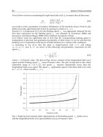
Environmental flows include natural phenomena such as atmospheric weather patterns and ocean currents (Fig. 2) and
flows of molten rock beneath the crust of the earth. Engineering design issues arise in the extraction of fossil fuels and
other materials from the earth, in bridge and building design, and in the treatment and dispersal of wastes from electrical

utilities, transportation systems and vehicles, and industrial manufacturing plants. Such problems typically are
characterized by a coupling of natural convection (resulting from temperature and/or concentration gradients) with other
forces, in many cases including the rotation of the earth.
Internal Combustion Engine. The final example shows a few results from transient computations of flow, fuel spray,
and combustion in a reciprocating internal combustion engine (Fig. 11) (Ref 74, 75). This application includes geometric
complexity (complex internal flow passages, moving boundaries piston and valves), physical complexity (turbulence,
combustion, multiphase flow), and numerical challenges (deforming mesh, large density and fluid property variations,
coupled Eulerian/Lagrangian algorithms). This represents an application area of CFD that lies at the frontier between
research and engineering application.

Fig. 11 Examples of CFD for in-
cylinder processes reciprocating IC engines. (a) Instantaneous computed and
measured induction flow at piston bottom-dead-
center for a port and chamber configuration yielding weakly
structured in-cylinder flow (Ref 74
). (b) Instantaneous computed and measured induction flow at piston
bottom-dead-center for a port and chamber configuration yielding a highly structured in-cylinder flow (Ref 74
).
(c) Instantaneous computed velocity field and flame propagation near piston top-dead-
center for a production
four-valve-per-cylinder engine. (d) Instantaneous computed fuel spray for a direct-injection diesel engine (
Ref
75). (e) Computed and measured heat release for a direct-injection diesel engine (Ref 75)
Of particular interest in a homogeneous-charge spark-ignited engine is the trade-off between flow losses and in-cylinder
flow "structure." Flow losses (induction system pressure drop) reduce the quantity of air that can be drawn into the
cylinder, lowering engine peak power. A coherent large-scale in-cylinder flow structure tends to yield higher combustion
efficiency, but generation of highly structured flow (e.g., a large-scale swirl about the cylinder axis) generally implies a
pressure-drop penalty. These trade-offs can be quantified and optimized using CFD (Ref 74). The computations of Fig.
11(a) and 11(b) were performed on unstructured meshes of up to 250,000 predominantly hexahedral cells; computation
through one crankshaft revolution required about 150 equivalent single-processor Cray YMP CPU hours.

Flame propagation for a production four-valve-per-cylinder automotive engine is shown in Fig. 11(c). Flame shapes and
burn rates are tailored by changing the intake port, intake valve, and combustion chamber geometry. A good design
generally is one having favorable spark-gap conditions and a flame that propagates uniformly outward to reach all solid
walls at the same instant.
Direct-injection diesel and gasoline engines, wherein liquid fuel is injected directly into the combution chamber, are of
interest for their high fuel economy potential. Here mixing and fuel stratification are key issues affecting combustion
performance; CFD is one tool that is being used to explore the influence of flow structure, injector placement, and
injection characteristics on engine combustion performance (Fig. 11d, e) (Ref 75).

References cited in this section
27.

D.C. Wilcox, Turbulence Modeling for CFD, DCW Industries, 1993
32.

C.A.J. Fletcher, Computational Techniques for Fluid Dynamics,
Vol II, Specific Techniques for Different
Flow Categories, 2nd ed., Springer-Verlag, 1991
46.

M.C. Cline, J.K. Dukowicz, and F.L. Addessio, "CAVEAT-GT: A General Topology Version of
the
CAVEAT Code," report LA-11812-MS, Los Alamos National Laboratory, June 1990
47.

HEXAR, Cray Research Inc., 1994
48.

G.D. Sjaardeam et al., CUBIT Mesh Generation Environment, Vol 1 & 2, SAND94-1100/-
1101 Sandia

National Laboratories, 1994
52.

M. Landon and R. Johnson, Idaho National Engineering Laboratory, 1995
53.

S. Ashley, Rapid Concept Modelers, Mech. Eng., Vol 118 (No.1), Jan 1996, p 64-66
54.

D.L. Reuss, R.J. Adrian, C.C. Landreth, D.T. French, and T.D. Fansler, "Instantaneous Planar
Measurements of Velocity and Large-
Scale Vorticity and Strain Rate Using Particle Image Velocimetry,"
Paper 890616, SAE, 1989
55.

M.C. Drake, T.D. Fansler, and D.T. French, "Crevice Flow and Combustion Visualization in a Direct-
Injection Spark-Ignition Engine Using Laser Imaging Techniques," Paper 952454, SAE International, 1995
56.

D. Deitz, Next-Generation CAD Systems, Mech. Eng., Vol 118 (No.8), Aug 1996, p 68-72
57.

G. Farin, Curves and Surfaces for Computer-Aided Geometric Design, Academic Press, 1990
58.

M. Hosaka, Modeling of Curves and Surfaces in CAD/CAM, Springer-Verlag, 1992
59.

D.C. Chan, A Least Squares Spectral Element Method for Incompressible Flow Simulations,
Proceedings

of the Fifteenth International Conference on Numerical Methods in Fluid Dynamics, Springer-Verlag, 1996

60.

"3D Piping IGES Application Protocol Version 1.2," IGES 5.2 Standard, IGES ANS US PRO/IPO-100-
1993, U.S. Product Data Association, 1993
61.

S. Sengupta, J. Hauser, P.R. Eiseman and J.F.Thompson, Ed. Numerical Grid Generat
ion in Computational
Fluid Dynamics, Pineridge Press, 1988
62.

D.C. Haworth, S.H. El Tahry, and M.S. Huebler, A Global Approach to Error Estimation and Physical
Diagnostics in Multidimensional Computational Fluid Dynamics, Int. J. Numer. Methods Fluids, V
ol 17,
1993, p 75-97
63.

C
H. Lin, T. Han and V. Sumantran, Experimental and Computational Studies of Flow in a Simplified
HVAC Duct, Int. J. Vehicle Design, Vol 15 (No. 1/2), 1994, p 147-165
64.

FLUENT User's Group meeting, FLUENT Inc. (Lebanon, NH), 1995
65.

T. Han, D.C. Hammond, and C.J. Sagi, Optimization of Bluff Body for Minimum Drag in Ground
Proximity, AIAA J., Vol 30 (No.4). April 1992, p 882-889
66.

M.B. Malone, W.P. Dwyer, and D. Crouse, "A 3D Navier-Strokes Analysis of Generic Ground Vehicl
e
Shape," Paper No. AIAA-93-3521-CP, American Institute of Aeronautics and Astronautics, 1993
67.

T. Han, Computational Analysis of Three-
Dimensional Turbulent Flow around a Bluff Body in Ground
Proximity, AIAA J., Vol 27 (No. 9), Sept 1989, p 1213-1219
68.

T. Han, V. Sumantran, C. Harris, T. Kuzmanov, M. Huebler, and T. Zak, "Flowfield Simulations of Three
Simplified Vehicle Shapes and Comparisons with Experimental Measurements," Paper 960678, SAE
International, 1996
69.

CFD Research Corporation, Huntsville, AL, 1995
70.

MAGMASOFT, developed by MAGMA Giessereitechnologie GmbH, Aachen, Germany; marketed and
supported in the U.S. by MAGMA Foundry Technologies, Inc., Arlington Heights, IL
71.

R.H. Box and L.H. Kallien, Simulation-Aided Die and Process Design, Die Cast. Eng., Sept/Oct 1994
72.

L. Karlsson, Computer Simulation Aids V-Process Steel Casting, Mod. Cast., Feb 1996
73.

Fluid Dynamics International, Evanston, IL, 1995

74.

B. Khalighi, S.H. El Tahry, D.C. Haworth, and M.S. Huebler, "Computation
and Measurement of Flow and
Combustion in a Four-Valve Engine with Intake Variations," Paper 950287, SAE International, 1995
75.

S. Kong, Z. Han, and R.D. Reitz, "The Development and Application of a Diesel Ignition and Combustion
Model for Multidimensional Engine Simulation," Paper 950278, SAE International, 1995
Computational Fluid Dynamics
Peter J. O'Rourke, Los Alamos National Laboratory; Daniel C. Haworth and Raj Ranganathan, General Motors Corporation

Issues and Directions for Engineering CFD
Geometric fidelity between hardware and the computational mesh is crucial to obtaining accurate results. It is
characteristic of the highly nonlinear flow equations that small geometric perturbations can result in large changes to the
flowfield. One example is shown in Fig. 12 (Ref 76). There, significantly different flow structure and mixing result when
the fraction-of-a-millimeter gap between piston and cylinder liner (the "top-ring-land crevice") is included in the mesh
compared to when it is ignored. With a top-ring-land crevice, the flow entering the cylinder attaches to the cylinder wall
and flows parallel to the wall for an extended time; in the absence of a top-ring-land crevice, the entering flow quickly
adopts the port angle on entering the cylinder. This highlights the importance of maintaining a consistent three-
dimensional representation of the hardware at all stages of design, analysis, and fabrication. The CFD practitioner should
be wary of compromising the geometry in favor of grid-generation expediency, particularly in applications where he or
she has little previous experience.

Fig. 12 Computed and measured ensemble-mean velocity fields on two-
dimensional cutting planes at 125°
after piston top-dead-center for a ported two-stroke-
cycle engine. Computational results with and without a
top-ring-land crevice are shown. (a) Measured. (b) CFD with top-ring-land crevice. (c) CFD without top-ring-
land crevice

Numerical Inaccuracy. Meshes of hundreds of thousands of computational cells are common in transient engineering
applications of CFD today, and several millions of cells are being used in steady-state computations. Even so, numerical
inaccuracy remains an issue for three-dimensional CFD. A mesh of 1 million cells corresponds to just 100 nodes in each
coordinate direction in a three-dimensional calculation. With the low-order numerics that characterize engineering CFD,
this is sufficient to resolve a dynamic range of about one order of magnitude (a factor of 10) in flow scales.
Rapid progress is being made both in discretization schemes for tetrahedral meshes, and in automated grid generation for
(primarily) hexahedral meshes; it is unclear at this time which will become dominant in engineering CFD.
The physical models used to represent turbulence, combustion, sprays, and other unresolvable phenomena are a third
source of uncertainty in CFD. Turbulence modeling, in particular, is an issue that affects nearly all engineering
applications. Research toward improved models continues. Much new physical insight into turbulence is itself being
derived from large-scale numerical simulations (Ref 77).
In many high-Reynolds-number engineering applications where the instantaneous flow is highly transient and three-
dimensional, turbulence models can be used to reduce the problem to one of steady flow, provided that the mean
quantities of interest are time independent. This reduces the computational requirements considerably and provides results
of acceptable accuracy in many cases. However, as engineering design requirements tighten, there is an increasing
number of problems that demand a full three-dimensional transient treatment. Models still are needed to account for
scales smaller than those that can be resolved numerically, but subgrid-scale turbulence models are used instead of
Reynolds-averaged models. The resulting three-dimensional time-dependent simulations in this case are referred to as
large-eddy simulations (LES) (Ref 78). The use of LES in engineering design is expected to proliferate rapidly. Examples
of current applications of interest include acoustics and aerodynamic noise (Ref 79) and in-cylinder flows in engines (Ref
80).
Each of these three sources of uncertainty can in principle be isolated and quantified in simple configurations where a
second source of data (e.g., experimental measurements) is available. It is more difficult in engineering applications of
CFD to isolate and to quantify these errors to obtain meaningful estimates of error bounds. Early in the history of three-
dimensional CFD, discrepancies between CFD and experiments generally were attributed to the turbulence model. The
importance of the other sources of uncertainty and numerical inaccuracy in particular, has been more widely
acknowledged recently (Ref 62, 81, 82). In the authors' experience, most discrepancies between computations and
measurements for single-phase nonreacting flows in complex configurations are traced to geometric infidelity or to
inadequate mesh resolution (in cases where they have been traced at all).
User Expertise. Computational fluid dynamics codes generally require more experience on the part of the user than

other, more mature, CAE tools (e.g., linear FEM structural analysis). "General-purpose" CFD software provides a large
number of numerical parameters and problem-specification options. In steady-flow problems, results should be
independent of the choice of initial conditions, but different initial conditions may lead to different steady solutions when
time-marching to the steady state. The choice of computational domain and specification of boundary conditions always
are important, both for steady and time-dependent flows. Minimal user experience may suffice to obtain a reliable
solution for steady incompressible flow in a benign geometric configuration, but considerable expertise is needed in
problem specification and in results interpretation for complex flows.
CFD and Experimental Measurements. The engineering and scientific community typically accepts measurements
from experiments as being more reliable than similar information generated by a CFD calculation. This is the reason for
the strong emphasis placed by the profession on "validating" CFD results. While it is true that there are many sources of
uncertainty in CFD, the same is true of experiments, particularly for complex systems (e.g., the in-cylinder flow in the last
example). When comparing CFD results with measurements for such complex engineering problems, it is more
appropriate to approach the exercise as a "reconciliation" rather than a "validation," as the latter implies that the
experiment provides the "correct" value.
Interdisciplinary Analysis. In this overview, CFD has been considered as an isolated analysis tool. This is
satisfactory only to the extent that one can reasonably prescribe boundary conditions that are independent of the flow
solution itself.
For example, in the coolant-flow analysis of Fig. 7(c) temperature boundary conditions might be prescribed from a
separate finite-element structural analysis, but the temperature field in the solid depends on the coolant flow itself. One
can alternate through a sequence of CFD and thermal structural analyses, taking the most recent boundary conditions
available at each step, to obtain a solution that effectively is coupled. A single direct computation of the coupled solution
would be more satisfactory, however. In this case, a coupled fluid/heat conduction analysis is feasible as many CFD codes
provide conjugate heat transfer capability.
More difficult are cases where fluids and solids interact in a manner that changes the shape of the flow domain.
Flow/structure interactions including deformations are important, for example, in some aircraft design problems or in
applications where there is significant thermal distortion. Interdisciplinary analysis tools are becoming available for these
problems and will see more widespread use in the future.
Future of Engineering CFD. Most contemporary commercial CFD codes start from a discretization of the continuum
equations of fluid mechanics and require a computational mesh of discrete cells or elements. An alternative is to approach
CFD from a kinetic theory point of view. In Ref 83, for example, an (essentially) grid-free Lagrangian-particle method

has been developed and implemented. It is too early, at the time of this writing, to speculate on the future of this approach
for engineering design. Computations have been reported for configurations including external flow over simplified and
realistic vehicles.
Active research areas for CFD include automated mesh generation, numerical algorithms for parallel computer
architectures, linear equation solvers, more accurate and stable discretization schemes, automatic numerical error
assessment and correction, improved solution algorithms for coupled nonlinear systems, new and enhanced physical
models, more sophisticated diagnostics, interdisciplinary coupled structures/fluids analysis, optimization algorithms, and
coupling of three-dimensional CFD into systems-level models.
In the ideal math-based design process, CFD is one part of a multidisciplinary CAE approach, and the full system (versus
isolated component) is considered. Grid generation is fully automated to ensure a high-quality (initial) mesh. The flow
solver selects all numerical parameters and provides automated solution-adaptive mesh refinement to a specified level of
error or allowable computational resource (time or cost). Solution diagnostics provide information of direct relevance to
the design requirements. Automated design optimization through modifications to the geometry and/or operating
conditions proceeds until design requirements are met.
While much work remains to realize this ideal, CFD already is being used with considerable success in engineering
design. Its utility and applicability will increase as the outstanding issues are resolved.
Sources for Further Information. Many references to specific topics have been cited throughout this chapter.
General CFD texts include Ref 3, 28, 31, and 32. At all stages of the CFD process (geometry acquisition, grid generation,
flow solution, and postprocessing), a broad array of commercial, public-domain, and in-house proprietary codes are being
used in engineering design. A small sampling of the software currently available to the design engineer has been
mentioned herein. For more comprehensive and up-to-date listings, the reader can consult several sources. Computer
hardware companies maintain lists of software that has been ported to their platforms; software vendors maintain lists of
codes with which their own products are compatible. Table 3 has been extracted from one such list (Ref 84). General (Ref
85) and industry-specific engineering periodicals often provide reviews of available software. And, a wealth of timely
information can be found on the Internet (Ref 86). Given the rapid pace at which CFD technology is evolving, this last
source is particularly valuable. In addition to lists and descriptions of the available software, user evaluations and direct
comparisons of alternative codes and methodologies can be found there.
Table 3 A partial listing of CFD data formats supported by one software vendor
This provides a snapshot in time (late 1996) of the wide variety of commercially available, public domain, and proprietary CFD
software used for engineering design and analysis.

Format/code name(s) Company
FLUENT/UNS, FLUENT-V4,
RAMPANT-V2 and V3, NEKTON,
TGRID
Fluent Inc., Lebanon, NH
GASP
AeroSoft, Inc., Blacksburg, VA
GMTEC
General Motors Corporation, Warren, MI
HAWK
California Institute of Technology, Pasadena, CA
Analytical Methods, Inc., Redmond, WA
INCA
Amtec Engineering, Inc., Bellevue, WA
KIVA-3, CHAD
Los Alamos National Laboratory, New Mexico
NASTAR
United Technologies Research Center, East Hartford, CT
NPARC Alliance, NASA Lewis Research Center and Arnold Engineering, Cleveland,
OH
NPARC
Sverdrup Technology, Inc./AEDC Group, Arnold AFB, TN
NS3D
Pratt & Whitney Canada, Longueil, Quebec, Canada
PAB3D
NASA Langley Research Center, Hampton, VA
PARC
NASA Ames Research Center & Boeing Co., NASA Amex Research Center, Moffett
Field, CA; Boeing Commercial Airplane Group, Propulsion Research CFD, Seattle, WA
PHOENICS

CHAM Ltd., Wimbledon Village, London, England
POLYFLOW
Polyflow S.A., Louvain-La-Neuve, Belgium
POLY3D
Rheotek, Inc., Montreal, Quebec, Canada
SPECTRUM-CENTRIC
CENTRIC Engineering Systems, Inc., Santa Clara, CA
STARCD
Computational Dynamics Ltd., London, England
TASCflow
Advanced Scientific Computing Ltd., Waterloo, Ontario, Canada
TEAM
Lockheed Aeronautical Systems Co., CA
TNS3Dmb
NASA Langley Research Center, Hampton, VA
TRANAIR
NASA Ames Research Center, Moffett Field, CA
UH3D
Ford Motor Co., Dearborn, MI
USAERO, VSAERO
Analytical Methods, Inc., Redmond, WA
Y237
United Technologies Research Center, East Hartford, CT
ACE-U, CFD-ACE
CFD Research Corporation, Huntsville, AL
AIRFLO3D
Texas Tech University, Department of Mechanical Engineering
ALPHA-FLOW
Fuji Research Institute, Japan
BAGGER

Eglin AFB, FL
CFD++
Metacomp Technologies, Inc., Westlake Village, CA
CFL3D
NASA Langley Research Center, Hampton, VA
CFX
AEA Technology Engineering Software, Inc., Bethel Park, PA
COMCO
The Computational Mechanics Company, Inc., Austin, TX
DSMC-SANDIA
Sandia National Laboratory, Albuquerque, NM
FASTU
NASA Langley Research Center, Hampton, VA
Fluent Inc. (bought FDI Ltd in 1996), Lebanon, NH
FIDAP
Fluid Dynamics International, Evanston, IL
FIRE
KIT Corporation, St. Paul, MN
FLEX
Sverdrup Technology, Inc., Eglin AFB, FL
FLOTRAN
Swanson Analysis Systems Inc., Houston, PA
Source: Ref 84
CFD is at a relatively early stage of development compared to other areas of CAE such as linear FEM structural analysis.
No single code covers all areas of application equally well. While "general-purpose" CFD has been emphasized here,
specialized application-specific numerical methods and software often are needed. Specialized experience and expertise
can be found within university engineering departments, U.S. national laboratories, and engineering consulting firms;
again, the Internet provides a good vehicle for exploring these possibilities.

References cited in this section

3. P.J. Roache, Computational Fluid Dynamics, Hermosa Publishers, 1982
28.

R. Peyret and T.D. Taylor, Computational Methods for Fluid Flow, Springer-Verlag, 1983
31.

C.A.J. Fletcher, Computational Techniques for Fluid Dynamics, Vol I,
Fundamental and General
Techniques, 2nd ed., Springer-Verlag, 1991
32.

C.A.J. Fletcher, Computational Techniques for Fluid Dynamics,
Vol II, Specific Techniques for Different
Flow Categories, 2nd ed., Springer-Verlag, 1991
62.

D.C. Haworth, S.H. El Tahry, and M.S. Huebler, A Global Approa
ch to Error Estimation and Physical
Diagnostics in Multidimensional Computational Fluid Dynamics, Int. J. Numer. Methods Fluids,
Vol 17,
1993, p 75-97
76.

D. C. Haworth, M.S. Huebler, S.H. El Tahry, and W. R. Matthes, Multidimensional Calculations for a Two-
Stroke-Cycle Engine: a Detailed Scavenging Model Validation, Paper 932712, SAE, 1993
77.

P. Moin and J. Kim, Tackling Turbulence with Supercomputers, Scientific American,
Vol 276 (No. 1), Jan
1997, p 62-68

78.

B. Galperin and S.A. Orszag, Ed., Large-Eddy Simulation of Complex Engineering and Geophysical Flows,

Cambridge University Press, 1993
79.

A.R. George, Automobile Aerodynamic Noise, SAE Trans., Vol 99-6, 1990, p 434-457
80.

D.C. Haworth and K. Jansen, LES on Unstructured Deforming Meshes: Towar
ds Reciprocating IC Engines,
Proceedings of the 1996 Summer Program,
Stanford University/NASA Ames Center for Turbulence
Research, 1996, p 329-346
81.

R.W. Johnson and E.D. Hughes, Ed., Quantification of Uncertainty in Computational Fluid Dynamics,

FED-Vol 213, Fluids Engineering Division, American Society of Mechanical Engineers, 1995
82.

I. Celik, C.J. Chen, P.J. Roache, and G. Scheuerer, Ed.,
Quantification of Uncertainty in Computational
Fluid Dynamics, FED-Vol 158, Fluids Engineering Division, Americ
an Society of Mechanical Engineers,
1993
83.

K. Molvig, Digital Physics: A New Technology for Fluid Simulation,

Exa Corporation, Cambridge, MA,
Aug 1993
84.

D. Poirier, ICEM CFD Engineering, personal communication, 1996
85.

D. Deitz, Designing with CFD, Mech. Eng., Vol 118 (No. 3), March 1996, p 90-94
86.

D. Deitz, Engineering Online, Mech. Eng., Vol 118 (No. 1), Jan 1996, p 84-88
Computational Fluid Dynamics
Peter J. O'Rourke, Los Alamos National Laboratory; Daniel C. Haworth and Raj Ranganathan, General Motors Corporation

References
1. FLOWMASTER USA, Inc. Fluid Dynamics International, Evanston, IL
2. WAVE Basic Manual: Documentation/User's Manual,
Version 3.4, Ricardo Software, Burr Ridge, IL, Oct
1996
3. P.J. Roache, Computational Fluid Dynamics, Hermosa Publishers, 1982
4.
N. Grün, "Simulating External Vehicle Aerodynamics with Carflow," Paper 960679, SAE International,
1996
5. W. Aspray, John von Neumann and the Origins of Modern Computing, MIT Press, 1990
6. "Accelerated Strategic Computing
Initiative (ASCI): Draft Program Plan," Department of Energy Defense
Program, May 1996
7. L.H. Turcotte, ICASE/LaRC Industry Roundtable, Oct 3-
4, 1994; original source for some data is F.
Baskett and J.L. Hennessey, Microprocessors: From Desktops to Supercomputers, Science,

Vol 261, 13
Aug 1993, p 864-871
8. J.K. Dukowicz and R.D. Smith, J. Geophys. Res., Vol 99, 1994, p 7991-8014
9. R.D. Smith, J.K. Dukowicz, and R.C. Malone, Physica D, Vol 60, 1992, p 38-61
10. G. Taubes, Redefining the Supercomputer, Science, Vol 273, Sept 1996, p 1655-1657
11. J.B. Heywood,Internal Combustion Engine Fundamentals, McGraw-Hill, 1988
12. F.H. Harlow and A.A. Amsden, "Fluid Dynamics," Report LA-
4700, Los Alamos Scientific Laboratory,
June 1971
13. W.G. Vincenti and C. H. Kruger, Introduction to Physical Gas Dynamics,
Robert E. Krieger Publishing,
1975
14. P.A. Thompson, Compressible-Fluid Dynamics, McGraw-Hill, 1972
15. H. Jeffreys, Cartesian Tensors, Cambridge University Press, 1997
16. F.A. Williams, Combustion Theory, 2nd ed., Benjamin/Cummings, 1985
17. T.G. Cowling, Magnetohydrodynamics, Interscience Tracts on Physics and Astronomy, No. 4, 1957
18. S. Chandrasekhar, Radiative Transfer, Dover, 1960
19. D.R. Stull and H. Prophet, JANAF Thermochemical Tables, 2nd ed., NSRDS-
NBS37, National Bureau of
Standards, 1971
20.
B. McBride and S. Gordon, "Computer Program for Calculating and Fitting Thermodynamic Functions,"
NASA-RP-1271, National Aeronautics and Space Administration, 1992
21. R.B. Bird, W. E. Stewart, and E.N. Lightfoot, Transport Phenomena, Wiley, 1960
22. L. Crocco, A. Suggestion for the Numerical Solution of the Steady Navier-Strokes Equations, AIAA J.,
Vol
3 (No. 10), 1965, p 1824-1832
23. L.D. Landau and E.M. Lifshitz, Fluid Mechanics, Pergamon Press, 1959
24.
O. Reynolds, On the Dynamical Theory of Incompressible Viscous Fluids and the Determination of the

Criterion, Philos. Trans. R. Soc. London, Series A, Vol 186, 1895, p 123
25. H. Tennekes and J.L. Lumley, A First Course in Turbulence, MIT Press, 1972
26. B.E. Launder and D.B. Spalding, Mathematical Models of Turbulence, Academic Press, 1972
27. D.C. Wilcox, Turbulence Modeling for CFD, DCW Industries, 1993
28. R. Peyret and T.D. Taylor, Computational Methods for Fluid Flow, Springer-Verlag, 1983
29. G.D. Smith, Numerical Solution of Partial Differential Equations, 2nd ed., Oxford University Press, 1978
30. R.D. Richtmyer and K.W. Morton, Difference Methods for Initial-Value Problems,
2nd ed., Interscience
Publishers, 1967
31. C.A.J. Fletcher, Computational Techniques for Fluid Dynamics, Vol I,
Fundamental and General
Techniques, 2nd ed., Springer-Verlag, 1991
32. C.A.J. Fletcher, Computational Techniques for Fluid Dynamics,
Vol II, Specific Techniques for Different
Flow Categories, 2nd ed., Springer-Verlag, 1991
33.
G.G. O'Brien, M.A. Hyman and S. Kaplan, A Study of the Numerical Solution of Partial Differential
Equations, J. Math. Phys., Vol 29, 1950, p 223-251
34. M.J. Lee and W.C. Reynolds, "Numerical Experiments on the Structure of
Homogeneous Turbulence,"
Report TF-24, Dept. of Mechanical Engineering, Stanford University, 1985
35. J.U. Brackbill and J.J. Monaghan, Ed.,
Proceedings of the Workshop on Particle Methods in Fluid
Dynamics and Plasma Physics, in Comput. Phys. Commun., Vol 48 (No. 1), 1988
36. F.H. Harlow, The Particle-in-Cell Computing Method for Fluid Dynamics,
Fundamental Methods in
Hydrodynamics, B. Alder, S. Fernbach and M. Rotenberg, Ed., Academic Press, 1964
37. J.U. Brackbill and H.M. Ruppel, FLIP: A Method for Adaptively Zoned, Particle-in-
Cell Calculations of
Fluid Flows in Two Dimensions, J. Comput. Physics, Vol 65, 1986, p 314

38. J.J. Monaghan, Particle Methods for Hydrodynamics, Comput. Phys. Rep., Vol 3, 1985, p 71-124
39. J.K. Dukowicz, A Particle-Fluid Numerical Model for Liquid Sprays, J. Comput. Phys.,
Vol 35 (No. 2),
1980, p 229-253
40.
P.J. O'Rourke, "Collective Drop Effects in Vaporizing Liquid Sprays," Ph.D. thesis, Princeton University,
1981
41. Y. Sahd and M. Schultz, Conjugate Gradient-like Algorithms for Solving Non-
Symmetric Linear Systems,
Math. Comput., Vol 44, 1985, p 417-424
42. W.L. Briggs, A Multigrid Tutorial, Society for Industrial and Applied Mathematics (Philadelphia), 1987
43. W.H. Press, B.P. Flannery, S.A. Teukolsky, and W.T. Vettering
Numerical Recipes: The Art of Scientific
Computing, Cambridge University Press, 1987
44. D.A.Knoll and P.R. McHugh, Newton-Krylov Methods Applied to a System of Convection-Diffusion-
Reaction Equations, Compt. Phys. Commun., Vol 88, 1995, p 141-160
45. S.V. Patankar, Numerical Heat Transfer and Fluid Flow, McGraw-Hill, 1980
46. M.C. Cline, J.K. Dukowicz, and F.L. Addessio, "CAVEAT-
GT: A General Topology Version of the
CAVEAT Code," report LA-11812-MS, Los Alamos National Laboratory, June 1990
47. HEXAR, Cray Research Inc., 1994
48. G.D. Sjaardeam et al., CUBIT Mesh Generation Environment, Vol 1 & 2, SAND94-1100/-
1101 Sandia
National Laboratories, 1994
49. W.D. Henshaw, A Fourth-Order Accurate Method for the Incompressible Navier-Stokes Equatio
ns on
Overlapping Grids, J. Comput. Phys., Vol 133, 1994, p 13-25
50.
R.B. Pember, et al., "An Embedded Boundary Method for the Modeling of Unsteady Combustion in an
Industrial Gas-Fired Furnace," Report UCRL-JC-122177, Lawrence Livermore National Laborat

ory, Oct
1995
51.
J.P. Jessee, et al., "An Adaptive Mesh Refinement Algorithm for the Discrete Ordinates Method," Report
LBNL-38800, Lawrence Berkely National Laboratory, March 1996
52. M. Landon and R. Johnson, Idaho National Engineering Laboratory, 1995
53. S. Ashley, Rapid Concept Modelers, Mech. Eng., Vol 118 (No.1), Jan 1996, p 64-66
54.
D.L. Reuss, R.J. Adrian, C.C. Landreth, D.T. French, and T.D. Fansler, "Instantaneous Planar
Measurements of Velocity and Large-Scale Vorticity and Strain Rate Usi
ng Particle Image Velocimetry,"
Paper 890616, SAE, 1989
55. M.C. Drake, T.D. Fansler, and D.T. French, "Crevice Flow and Combustion Visualization in a Direct-
Injection Spark-Ignition Engine Using Laser Imaging Techniques," Paper 952454, SAE International,

1995
56. D. Deitz, Next-Generation CAD Systems, Mech. Eng., Vol 118 (No.8), Aug 1996, p 68-72
57. G. Farin, Curves and Surfaces for Computer-Aided Geometric Design, Academic Press, 1990
58. M. Hosaka, Modeling of Curves and Surfaces in CAD/CAM, Springer-Verlag, 1992
59. D.C. Chan, A Least Squares Spectral Element Method for Incompressible Flow Simulations,
Proceedings
of the Fifteenth International Conference on Numerical Methods in Fluid Dynamics, Springer-
Verlag,
1996
60. "3D Piping IGES Application Protocol Version 1.2," IGES 5.2 Standard, IGES ANS US PRO/IPO-100-
1993, U.S. Product Data Association, 1993
61. S. Sengupta, J. Hauser, P.R. Eiseman and J.F.Thompson, Ed.
Numerical Grid Generation in
Computational Fluid Dynamics, Pineridge Press, 1988
62.

D.C. Haworth, S.H. El Tahry, and M.S. Huebler, A Global Approach to Error Estimation and Physical
Diagnostics in Multidimensional Computational Fluid Dynamics, Int. J. Numer. Methods Fluids,
Vol 17,
1993, p 75-97
63. C H. Lin, T. Han and V. Sumantran,
Experimental and Computational Studies of Flow in a Simplified
HVAC Duct, Int. J. Vehicle Design, Vol 15 (No. 1/2), 1994, p 147-165
64. FLUENT User's Group meeting, FLUENT Inc. (Lebanon, NH), 1995
65. T. Han, D.C. Hammond, and C.J. Sagi, Optimization of
Bluff Body for Minimum Drag in Ground
Proximity, AIAA J., Vol 30 (No.4). April 1992, p 882-889
66. M.B. Malone, W.P. Dwyer, and D. Crouse, "A 3D Navier-
Strokes Analysis of Generic Ground Vehicle
Shape," Paper No. AIAA-93-3521-CP, American Institute of Aeronautics and Astronautics, 1993
67. T. Han, Computational Analysis of Three-
Dimensional Turbulent Flow around a Bluff Body in Ground
Proximity, AIAA J., Vol 27 (No. 9), Sept 1989, p 1213-1219
68. T. Han, V. Sumantran, C. Harris, T. Kuzmanov, M. Huebler,
and T. Zak, "Flowfield Simulations of Three
Simplified Vehicle Shapes and Comparisons with Experimental Measurements," Paper 960678, SAE
International, 1996
69. CFD Research Corporation, Huntsville, AL, 1995
70. MAGMASOFT, developed by MAGMA Giessereite
chnologie GmbH, Aachen, Germany; marketed and
supported in the U.S. by MAGMA Foundry Technologies, Inc., Arlington Heights, IL
71. R.H. Box and L.H. Kallien, Simulation-Aided Die and Process Design, Die Cast. Eng., Sept/Oct 1994
72. L. Karlsson, Computer Simulation Aids V-Process Steel Casting, Mod. Cast., Feb 1996
73. Fluid Dynamics International, Evanston, IL, 1995
74.
B. Khalighi, S.H. El Tahry, D.C. Haworth, and M.S. Huebler, "Computation and Measurement of Flow

and Combustion in a Four-Valve Engine with Intake Variations," Paper 950287, SAE International, 1995
75.
S. Kong, Z. Han, and R.D. Reitz, "The Development and Application of a Diesel Ignition and Combustion
Model for Multidimensional Engine Simulation," Paper 950278, SAE International, 1995
76.
D. C. Haworth, M.S. Huebler, S.H. El Tahry, and W. R. Matthes, Multidimensional Calculations for a
Two-Stroke-Cycle Engine: a Detailed Scavenging Model Validation, Paper 932712, SAE, 1993
77. P. Moin and J. Kim, Tackling Turbulence with Supercomputers, Scientific American,
Vol 276 (No. 1), Jan
1997, p 62-68
78. B. Galperin and S.A. Orszag, Ed., Large-
Eddy Simulation of Complex Engineering and Geophysical
Flows, Cambridge University Press, 1993
79. A.R. George, Automobile Aerodynamic Noise, SAE Trans., Vol 99-6, 1990, p 434-457
80.
D.C. Haworth and K. Jansen, LES on Unstructured Deforming Meshes: Towards Reciprocating IC
Engines, Proceedings of the 1996 Summer Program,
Stanford University/NASA Ames Center for
Turbulence Research, 1996, p 329-346
81. R.W. Johnson and E.D. Hughes, Ed., Quantification of Uncertainty in Computational Fluid Dynamics,

FED-Vol 213, Fluids Engineering Division, American Society of Mechanical Engineers, 1995
82. I. Celik, C.J. Chen, P.J. Roache, and G. Scheuerer, Ed., Quanti
fication of Uncertainty in Computational
Fluid Dynamics, FED-
Vol 158, Fluids Engineering Division, American Society of Mechanical Engineers,
1993
83. K. Molvig, Digital Physics: A New Technology for Fluid Simulation,
Exa Corporation, Cambridge, MA,
Aug 1993

84. D. Poirier, ICEM CFD Engineering, personal communication, 1996
85. D. Deitz, Designing with CFD, Mech. Eng., Vol 118 (No. 3), March 1996, p 90-94
86. D. Deitz, Engineering Online, Mech. Eng., Vol 118 (No. 1), Jan 1996, p 84-88
Computer-Aided Electrical/Electronic
Design
Shaun S. Devlin, Ford Motor Company

Introduction