Dynamics of Mechanical Systems 2009 Part 5 pps

182 Dynamics of Mechanical Systems
By eliminating S
A
and S
B
between these three equations, we have:
(6.7.13)
Now, suppose that
A
is represented by a single force, say F
A
, passing through some
common point C of A and B (or A and B extended) together with a couple with torque
T
A
. Similarly, let
B
be represented by a single force F
B
passing through C together with
a couple with torque T
B
. Then, because
A
and
B
taken together form a zero system (Eq.
(6.7.3)), the resultant of
A
and
B

and the moment of
A
and
B
about C must be zero.
That is,
(6.7.14)
and
(6.7.15)
Equations (6.7.13), (6.7.14), and (6.7.15), or the equivalent wording, represent the law of
action and reaction.
6.8 First Moments
Consider a particle P with mass m (or, alternatively, a point P with associated mass m) as
depicted in Figure 6.8.1. Let O be an arbitrary reference point, and let p be a position
vector locating P relative to O. The first moment of P relative to O, φ
P/O
, is defined as:
(6.8.1)
Consider next a set S of N particles P
i
(i = 1,…, N) having masses as in Figure 6.8.2,
where O is an arbitrary reference point. The first moment of S for O, φ
S/O
, is defined as
the sum of the first moments of the individual particles of S for O. That is,
(6.8.2)
Observe that, in general, φ
S/O
is not zero. However, if a point G can be found such that the
first moment of S relative to G, φ

S/G
, is zero, then G is defined as the mass center of S.
Using this definition, the existence and location of G can be determined from Eq. (6.8.2).
Specifically, if G is the mass center and if r
i
locates p
i
relative to G, as in Figure 6.8.3, then
the first moment of S relative to G may be expressed as:
(6.8.3)
ˆˆ
SS
AB
+=0
ˆ
S
ˆ
S
ˆ
S
ˆ
S
ˆ
S
ˆ
S
ˆ
S
ˆ
S

FF F F
AB A B
+= =−0 or
TT T T
AB A B
+= =−0 or
φ
PO
D
m= p
φ
SO
D
NN ii
i
N
=+++=
=
∑
mp mp m p mp
11 22
1
K
φ
SG
ii
i
N
m==
=

∑
r
1
0
0593_C06_fm Page 182 Monday, May 6, 2002 2:28 PM
Forces and Force Systems 183
From Figure 6.8.3, we have:
(6.8.4)
Hence, by substituting into Eq. (6.8.3), we obtain:
(6.8.5)
By solving the last equation for p
G
, we obtain:
(6.8.6)
where M is the total mass of S. That is,
(6.8.7)
FIGURE 6.8.1
A particle P and reference point O.
FIGURE 6.8.2
A set S of particles and a reference point O.
FIGURE 6.8.3
A set S of particles with mass center G.
p
O
P(m)
p
P (m )
P (m )
P (m )
P (m )

O
1 1
2
2
i i
N
N
i
S
p
P (m )
P (m )
P (m )
O
1 1
2
2
i i
i
S
G
r
i
p
G
pp r rpp
iGi iiG
=+ =− or
mm
mm

mm
ii
i
N
ii G
i
N
ii iG
i
N
i
N
ii i
i
N
i
N
G
rpp
pp
pp
==
==
==
∑∑
∑∑
∑∑
=−
()
=−

=−






=
11
11
11
0
pp
Gii
i
N
Mm=
()
=
∑
1
1
Mm
i
i
N
=
=
∑
1

0593_C06_fm Page 183 Monday, May 6, 2002 2:28 PM
184 Dynamics of Mechanical Systems
Equation (6.8.6) demonstrates the existence of G by providing an algorithm for its location.
We may think of a body as though it were composed of particles, just as a sandstone is
composed of particles of sand. Then, the sums in Eqs. (6.8.2) through (6.8.7) become very
large, and in the limit they may be replaced by integrals.
For homogeneous bodies, the mass is uniformly distributed throughout the region, or
geometric figure, occupied by the body. The mass center location is then solely determined
by the shape of the figure of the body. The mass center position is then said to be at the
centroid of the geometric figure of the body. The centroid location for common and simple
geometric figures may be determined by routine integration. The results of such integra-
tions are listed in figurative form in Appendix I. As the name implies, a centroid is at the
intuitive center or middle of a figure.
As an illustration of these concepts, consider the gravitational forces acting on a body
B with an arbitrary shape. Let B be composed of N particles P
i
having masses m
i
(i = 1,…, N), and let G be the mass center of B, as depicted in Figure 6.8.4.
Let the set of all the gravitational forces acting on B be replaced by a single force W
passing through G together with a couple with torque T. Then, from the definition of
equivalent force systems, W and T are:
(6.8.8)
and
(6.8.9)
where k is a downward-directed unit vector as in Figure 6.8.4 and M is the total mass of
particles of B. The last equality of Eq. (6.8.9) follows from the definition of the mass center
in Eq. (6.8.3).
Equations (6.8.7) and (6.8.8) show how dramatic the reduction in forces can be through
the use of equivalent force systems.

6.9 Physical Forces: Inertia (Passive) Forces
Inertia forces arise due to acceleration of particles and their masses. Specifically, the inertia
force on a particle is proportional to both the mass of the particle and the acceleration of
FIGURE 6.8.4
Gravitational forces on the particles
of a body.
1
i
S
P
P
G
k
m g
m g
m g
i
1
r
i
2
P
2
Wk kk==







=
==
∑∑
mg m g Mg
i
i
N
i
i
N
11
Trk rk=×=






×=
==
∑∑
ii
i
N
ii
i
N
mg m g
11
0

0593_C06_fm Page 184 Monday, May 6, 2002 2:28 PM
Forces and Force Systems 185
the particle. However, the inertia force is directed opposite to the acceleration. Thus, if P
is a particle with mass m and with acceleration a in an inertial reference frame R, then the
inertia force F
*
exerted on P is:
(6.9.1)
An inertial reference frame is defined as a reference frame in which Newton’s laws of
motion are valid. From elementary physics, we recall that from Newton’s laws we have
the expression:
(6.9.2)
where F represents the resultant of all applied forces on a particle P having mass m and
acceleration a. By comparing Eqs. (6.9.1) and (6.9.2), we have:
(6.9.3)
Equation (6.9.3) is often referred to as d’Alembert’s principle. That is, the sum of the
applied and inertia forces on a particle is zero. Equation (6.9.3) thus also presents an
algorithm or procedure for the analysis of dynamic systems as though they were static
systems.
For rigid bodies, considered as sets of particles, the inertia force system is somewhat
more involved than for that of a single particle due to the large number of particles making
up a rigid body; however, we can accommodate the resulting large number of inertia
forces by using equivalent force systems, as discussed in Section 6.5. To do this, consider
the representation of a rigid body as a set of particles as depicted in Figure 6.9.1. As B
moves in an inertial frame R, the particles of B will be accelerated and thus experience
inertia forces; hence, the inertia force system exerted on B will be made up of the inertia
forces on the particles of B. The inertia force exerted on a typical particle P
i
of B is:
(6.9.4)

where m
i
is the mass of P
i
and A
i
is the acceleration of P
i
in R.
Using the procedures of Section 6.5, we can replace this system of many forces by a
single force F
*
passing through an arbitrary point, together with a couple having a torque
FIGURE 6.9.1
Representation of a rigid body as a
set of particles.
Fa
*
=−m
Fa= m
FF+=
*
0
Fa
iii
m
*
=−
P (m )
P (m )

P (m )
1 1
2
2
N
N
i
B
r
P (m )
i i
R
0593_C06_fm Page 185 Monday, May 6, 2002 2:28 PM
186 Dynamics of Mechanical Systems
T
*
. It is generally convenient to let F
*
pass through the mass center G of the body. Then,
F
*
and T
*
are:
(6.9.5)
and:
(6.9.6)
where r
i
locates P

i
relative to G.
Using Eq. (4.9.6), we see that because both P
i
and G are fixed on B, a
i
may be expressed as:
(6.9.7)
where αα
αα
and ωω
ωω
are the angular acceleration and angular velocity of B in R. Hence, by
substituting into Eq. (6.9.5), F* becomes:
(6.9.8)
or
(6.9.9)
where M is the total mass of B and where the last two terms of Eq. (6.9.8) are zero because
G is the mass center of B (see Eq. (6.8.3)).
Similarly, by substituting for a
i
in Eq. (6.9.6), T
*
becomes:
(6.9.10)
Fa
*
=−
()
=

∑
m
ii
i
N
1
Tra
*
=×−
()
=
∑
iii
i
N
m
1
aa r r
iG i i
=+×+××
()
ααωωωω
Farr
ar r
a
*
=− +×+××
()
[]
=−







−×
()
−× ×
()








=− − × − × ×
()
=
== =
∑
∑∑ ∑
m
mm m
M
iG i i
i
N

i
i
N
Gii
i
N
ii
i
N
G
ααωωωω
ααωωωω
ααωωωω
1
11 1
00
Fa=−M
G
Tr ar r
ra r r r r
arr r
*
=×−
()
+×+× ×
()
[]
=−







×− ××
()
−×××
()
[]
=− × − × ×
()
−×
=
== =
∑
∑∑ ∑
ii
i
N
Gi i
ii
i
N
Giii
i
N
ii i
i
N
Giii ii

m
mm m
mm
1
11 1
0
ααωωωω
ααωωωω
ααωω×××
()
==
∑∑
ωω r
i
i
N
i
N
11
0593_C06_fm Page 186 Monday, May 6, 2002 2:28 PM
Forces and Force Systems 187
or
(6.9.11)
where the first term of Eq. (6.9.10) is zero because G is the mass center, and the last term
is obtained from its counterpart in the previous line by using the identity:
(6.9.12)
To see this, simply expand the triple products of Eq. (6.9.10) using the identity. Specifically,
(6.9.13)
and
(6.9.14)

where the first terms are zero because r
i
and ωω
ωω
are perpendicular to ωω
ωω
× r
i
. Comparing
Eqs. (6.9.13) and (6.9.14), we see the results are the same. That is,
(6.9.15)
Neither of the terms of Eq. (6.9.11) is in a form convenient for computation or analysis;
however, the terms have similar forms. Moreover, we can express these forms in terms of
the inertia dyadic of the body as discussed in the next chapter. This, in turn, will enable us
to express T
*
in terms of the moments and products of inertia of B for its mass center G.
References
6.1. Kane, T. R., Analytical Elements of Mechanics, Vol. 1, Academic Press, New York, 1961, p. 150.
6.2. Kane, T. R., Dynamics, Holt, Rinehart & Winston, New York, 1968, pp. 92–115.
6.3. Huston, R. L., Multibody Dynamics, Butterworth-Heinemann, Stoneham, MA, 1990, pp. 153–212.
Problems
Section 6.2 Forces and Moments
P6.2.1: A force F with magnitude 12 lb acts along a line L passing through points P and
Q as in Figure P6.2.1. Let the coordinates of P and Q relative to a Cartesian reference frame
be as shown, measured in feet. Express F in terms of unit vectors n
x
, n
y
, and n

z
, which are
parallel to the X-, Y-, and Z-axes.
Trr rr
*
=××
()








−× × ×
()








∑∑
mm
ii i
i
N

ii i
i
N
ααωωωω
====11
abc acbabc××
()
≡⋅
()
−⋅
()
r rrrrrrr
i iiiiiii
×××
()
[]
=⋅ ×
()
−⋅
()
×=−⋅
()
×ωωωωωωωωωωωωωωωω
ωωωωωωωωωωωωωωωω×××
()
[]
=⋅ ×
()
−⋅
()

×=− ⋅
()
×r r rr rr rr
i i ii ii ii
rrrr
iiii
×××
()
[]
=×× ×
()
[]
ωωωωωωωω
0593_C06_fm Page 187 Monday, May 6, 2002 2:28 PM
188 Dynamics of Mechanical Systems
P6.2.2: See Problem P6.2.1. Find the moment of F about points O, A, and B of Figure P6.2.1.
Express the results in terms of n
x
, n
y
, and n
z
.
P6.2.3: A force F with magnitude 52 N acts along diagonal OA of a box with dimensions
as represented in Figure P6.2.3. Express F in terms of the unit vectors n
1
, n
2
, and n
3

, which
are parallel to the edges of the box as shown.
P6.2.4: See Problem P6.2.3. Find the moment of F about the corners A, B, C, D, E, G, and
H of the box. Express the results in terms of n
1
, n
2
, and n
3
.
Section 6.3 Systems of Forces
P6.3.1: Consider the force system exerted on the box as represented in Figure P6.3.1. The
force system consists of ten forces with lines of action and magnitudes as listed in Table
P6.3.1. Let the dimensions of the box be 12 m, 4 m, and 3 m, as shown.
a. Express the forces F
1
,…, F
10
in terms of the unit vectors n
1
, n
2
, and n
3
shown in
Figure P6.3.1.
b. Find the resultant of the force system expressed in terms of n
1
, n
2

, and n
3
.
c. Find the moment of the force system about O (expressed in terms of n
1
, n
2
,
and n
3
).
FIGURE P6.2.1
A force F acting along a line L.
FIGURE P6.2.3
A force F acting along a box diagonal.
O
Z
Y
X
n
n
n
z
y
x
P(1,2,4)
Q(2,5,3)
B(0,3,0)
A(2,0,0)
F

L
n
n
n
1
2
3
F
C D
H
G
E
B
O
A
12m
4m
3m
0593_C06_fm Page 188 Monday, May 6, 2002 2:28 PM
Forces and Force Systems 189
P6.3.2: See Problem 6.3.1, and (a) find the moment of the force system about points C and
H, and (b) verify Eq. (6.3.6) for these results. That is, show that:
where R is the resultant of the force system.
P6.3.3: A cube with 2-ft sides has forces exerted upon it as shown in Figure P6.3.3. The
magnitudes and lines of action of these forces are listed in Table P6.3.3.
FIGURE P6.3.1
A force system exerted on a box.
TABLE P6.3.1
Forces, Their Magnitudes, and Lines of Action for the Force
System of Figure P6.3.1

Force Magnitude (N) Line of Action
F
1
18 BA
F
2
25 BO
F
3
30 AO
F
4
10 CB
F
5
12 OC
F
6
26 OG
F
7
20 DH
F
8
25 EO
F
9
16 DG
F
10

24 CD
FIGURE P6.3.3
Forces exerted on a cube.
n
n
n
A
H
F
F
F
F
F
F
F
F
F
F
B
O
C
D
E
3m
4m
12m
G
8
10
9

4
3
5
1
2
2
3
1
7
6
M M CH R
CH
=+×
A
2 ft
D
E
H
G B
C
O
F
F
F
F
F
F
n
n
n

2
6
5
4
3
1
1
2
3
0593_C06_fm Page 189 Monday, May 6, 2002 2:28 PM
190 Dynamics of Mechanical Systems
a. Determine the resultant R of this system of forces.
b. Find the moments of the force system about points C, H, E, and G.
Express the results in terms of the unit vectors n
1
, n
2
, and n
3
shown in Figure P6.3.3.
6.4 Special Force Systems: Zero Force Systems and Couples
P6.4.1: In Figure P6.4.1, the box is subjected to forces as shown. The magnitudes and
directions of the forces are listed in Table P6.4.1. Determine the magnitudes of forces F
1
,
F
3
, F
4
, F

5
, F
6
, and F
10
so that the system of forces on the box is a zero system.
TABLE P6.3.3
Forces, Their Magnitudes, and Lines of Action for the Force
System of Figure P6.3.3
Force Magnitude (lb) Line of Action
F
1
10 AB
F
2
10 GH
F
3
8 CB
F
4
8 GD
F
5
12 CD
F
6
12 EO
FIGURE P6.4.1
Force system exerted on a box.

TABLE P6.4.1
Forces, Their Magnitudes, and Lines of Action
for the Forces of Figure P6.4.1
Force Magnitude (N) Line of Action
F
1
10 AB
F
2
8 CB
F
3
8 AO
F
4
6 HG
F
5
7 GO
F
6
5 AE
F
7
10 GD
F
8
16 DB
F
9

12 HD
F
10
9 CO
F
11
26 OD
n
n
A
H
F
F
F
F
F
F
F
F
B
O
C
D
E
3m
4m
12m
G
8
9

4
3
5
1
2
2
3
6
n
1
F
10
F
F
11
7
0593_C06_fm Page 190 Monday, May 6, 2002 2:28 PM
Forces and Force Systems 191
P6.4.2: Three cables support a 1500-lb load as depicted in Figure P6.4.2. By considering
the connecting joint O of the cables to the load to be in static equilibrium and by recalling
that forces in cables are directed along the cable, determine the forces in each of the cables.
The location of the fixed ends of the cables (A, B, and C) are determined by their x, y, z
coordinates (measured in feet) as shown in Figure P6.4.2.
P6.4.3: Repeat Problem P6.4.2 if the load is 2000 lb.
P6.4.4: Repeat Problem P6.4.3 if the coordinates of the cable supports (A, B, and C) are
given in meters instead of feet.
P6.4.5: Show that the force system exerted on the box shown in Figure P6.4.5 is a couple.
The magnitudes and directions of the forces are listed in Table P6.4.5.
FIGURE P6.4.2
Cables OA, OB, and OC supporting

a vertical load.
FIGURE P6.4.5
Forces system exerted on a box.
TABLE P6.4.5
Forces, Their Magnitudes, and Lines of Action
for the Forces of Figure P6.4.5
Force Magnitude (N) Line of Action
F
1
8 OC
F
2
8 BA
F
3
15 BO
F
4
12 CB
F
5
10 GA
F
6
10 CD
F
7
15 HE
F
8

12 AO
Z
Y
X
O(0,0,0)
C(3,7,5)
B(-2,2,10)
A(6,-3,8)
1500 lb
A
H
F
F
F
F
O
C
D
E
G
8
4
3
5
2
6
1
F
F
7

B
F
F
60 cm
40 cm
30 cm
0593_C06_fm Page 191 Monday, May 6, 2002 2:28 PM
192 Dynamics of Mechanical Systems
P6.4.6: See Problem P6.4.5. Find the torque of the couple.
P6.4.7: See Problems P6.4.5 and P6.4.6. Find the moment of the force system about points
O, A, D, and G.
P6.4.8: Show that the magnitude of the torque of a simple couple (two equal-magnitude
but oppositely directed forces) is simply the product of the magnitude of one of the forces
multiplied by the distance between the parallel lines of action of the forces. Show further
that the orientation of the torque is perpendicular to the plane of the forces, with sense
determined by the right-hand rule.
P6.4.9: Show that a set of simple couples is also a couple. Show further that the torque of
this composite couple is then simply the resultant (sum) of the torques of the simple
couples.
6.5 Equivalent Force Systems
P6.5.1: See Problem P6.3.1. Consider again the force system exerted on the box of Problem
P6.3.1 as shown in Figure P6.5.1, where the magnitudes and lines of action of the forces
are listed in Table P6.5.1. Suppose this force system is to be replaced by an equivalent
force system consisting of a single force F passing through O together with a couple having
torque T. Find F and T. (Express the results in terms of the unit vectors n
1
, n
2
, and n
3

of
Figure P6.5.1.)
FIGURE P6.5.1
A force system exerted on a box.
TABLE P6.5.1
Forces, Their Magnitudes, and Lines of Action
for the Force System of Figure P6.5.1
Force Magnitude (N) Line of Action
F
1
18 BA
F
2
25 BO
F
3
30 AO
F
4
10 CB
F
5
12 OC
F
6
26 OG
F
7
20 DH
F

8
25 EO
F
9
16 DG
F
10
24 CD
0593_C06_fm Page 192 Monday, May 6, 2002 2:28 PM
Forces and Force Systems 193
P6.5.2: Repeat Problem P6.5.1 with the single force F passing through G. Compare the
magnitudes of the respective couple torques.
P6.5.3: Consider a homogeneous rectangular block with dimensions a, b, and c as repre-
sented in Figure P6.5.3. Let the gravitational forces acting on the block be replaced by an
equivalent force system consisting of a single force W. If ρ is the uniform mass density of
the block, find the magnitude and line of action of W.
P6.5.4: See Problem P6.5.3. Suppose the gravitational force system on the block is replaced
by an equivalent force system consisting of a single force W passing through O together
with a couple with torque T. Find F and T. Express the results in terms of the unit vectors
n
1
, n
2
, and n
3
shown in Figure P6.5.3.
6.6 Wrenches
P6.6.1: See Problems P6.5.1 and P6.3.1. For the force system of Problems P6.5.1 and P6.3.1,
find the point Q
*

for which there is a minimum moment of the force system. Specifically,
find the position vector OQ
*
locating Q
*
relative to O. Express the result in terms of the
unit vectors n
1
, n
2
, and n
3
shown in Figure P6.5.1.
P6.6.2: See Problem P6.6.1. Find a wrench that is equivalent to the force system of Problems
P6.3.1, P6.5.1, and P6.6.1. Express the results in terms of the unit vectors of Figure P6.5.1.
6.7 Physical Forces: Applied (Active) Forces
P6.7.1: Suppose the human arm is modeled by three bodies B
1
, B
2
, and B
3
representing the
upper arm, lower arm, and hand, as shown in Figure P6.7.1A. Suppose further that the
FIGURE P6.5.3
A homogeneous rectangular block.
(A) (B)
FIGURE P6.7.1
(A) A model of the human arm. (B) Equivalent gravity (weight) forces on the human arm model.
n

n
n
1
2
3
O
a
b
c
0593_C06_fm Page 193 Monday, May 6, 2002 2:28 PM
194 Dynamics of Mechanical Systems
gravitational forces acting on these bodies are represented by equivalent gravity (weight)
force systems consisting of single vertical forces W
1
, W
2
, and W
3
as in Figure P6.7.1B.
Finally, suppose we want to find an equivalent gravity force system for the entire arm
consisting of a single force W passing through the shoulder joint O together with a couple
with torque M. Find W and M. Express the results in terms of the angles θ
1
, θ
2
, and θ
3
;
the distances r
1

, r
2
, r
3
, ᐉ
1
, ᐉ
2
, and ᐉ
3
; the force magnitudes W
1
, W
2
, and W
3
; and the unit
vectors n
x
, n
y
, and n
z
shown in Figures P6.7.1A and B.
P6.7.2: See Problem P6.7.1. Table P6.7.2 provides numerical values for the geometric
quantities and weights of the arm model of Figures P6.7.1A and B. Using these values,
determine the magnitudes of W and M.
P6.7.3: See Problems P6.7.1 and P6.7.2. Suppose the equivalent force system is to be a
wrench, where the couple torque M is a minimum. Locate a point G on the line of action
of the equivalent force. Find the magnitudes of the equivalent wrench force and minimum

moment.
P6.7.4: Three springs are connected in series as in Figure P6.7.4. Find the elongation for
the applied forces. The spring moduli and force magnitudes are listed in Table P6.7.4.
P6.7.5: See Problem P6.7.4. Let the springs of Problem P6.7.4 be arranged in parallel as in
Figure P6.7.5. Find the elongation δ for the applied forces. Assume that the springs are
sufficiently close (or even coaxial) so that the rotation of the attachment plates can be
ignored.
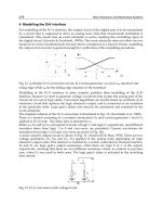
P6.7.6: A block is resting on an incline plane as shown in Figure P6.7.6. Let µ be the
coefficient of friction between the block and the plane. Find the inclination angle θ of the
incline where the block is on the verge of sliding down the plane.
P6.7.7: See Problem P6.7.6. Let the inclination angle θ be small. Let the drag factor (f) be
defined as an effective coefficient of friction that accounts for the small slope. Find f in
terms of µ and θ. What would be the value of f if the block is sliding up the plane?
TABLE P6.7.2
Numerical Values for the Geometric Parameters and Weights
of Figures P6.7.1A and B
i θθ
θθ
i
(°) r
i
(in.) ᐉ
i
(in.) W
i
(lb)
1 45 4.45 11.7 5.0
2 15 6.5 14.5 3.0
3 30 2.5 6.0 1.15
FIGURE P6.7.4

Three springs in series.
TABLE P6.7.4
Physical Data for the System of Figure P6.7.4
Force F Spring Moduli 12 lb (lb/in.) 50 N (N/mm)
k
1
610
k
2
512
k
3
87
F
F
k
k
1
2
k
3
0593_C06_fm Page 194 Monday, May 6, 2002 2:28 PM
Forces and Force Systems 195
P6.7.8: A homogeneous block is pushed to the right by a force P as in Figure P6.7.8. If
the friction coefficient between the block and plane is µ, find the maximum elevation
h above the surface where the force can be applied so that the block will slide and not tip.
P6.7.9: Figure P6.7.9 shows a schematic representation of a short-shoe drum brake. When
a force F is applied to the brake lever, the friction between the brake shoe and the drum
creates a braking force and braking moment on the drum. Let µ be the coefficient of friction
between the shoe and the drum. If the force F is known, determine the braking moment

M on the drum if the drum is rotating: (a) clockwise, and (b) counterclockwise. Express
M in terms of µ, F, and the dimensions a, b, c, d, and r shown in Figure P6.7.9.
P6.7.10: See Problem P6.7.9. Find a relation between µ and the dimensions of Figure P6.7.9
so that the brake is self-locking when the drum is rotating counterclockwise. (Self-locking
means that a negligible force F is required to brake the drum.)
FIGURE P6.7.5
Three springs in parallel.
FIGURE P6.7.6
Block on an inclined plane.
FIGURE P6.7.8
A block pushed along a surface.
FIGURE P6.7.9
A schematic representation of a brake
system.
F
F
k
k
1
2
k
3
θ
µ
µ
a
b
h
P
r

drum
brake shoe
b c
F
a
d
0593_C06_fm Page 195 Monday, May 6, 2002 2:28 PM
196 Dynamics of Mechanical Systems
Section 6.8 Mass Center
P6.8.1: Let a system of 10 particles P
i
(i = 1,…, 10) have masses m
i
and coordinates (x
i
, y
i
, z
i
)
relative to a Cartesian coordinate system as in Table P6.8.1. Find the coordinates
–
x,
–
y,
–
z
of the mass center of this set of particles if the m
i
are expressed in kilograms and the x

i
,
y
i
, z
i
are in meters. How does the result change if the m
i
are expressed in slug and the x
i
,
y
i
, z
i
in feet?
P6.8.2: See Problem P6.8.1. From the definition of mass center as expressed in Eq. (6.8.3)
show that the coordinates of the mass center may be obtained by the simple expressions:
where .
P6.8.3: Use the definition of mass center as expressed in Eq. (6.8.3) to show that the mass
center of a system of bodies may be obtained by: (a) letting each body B
i
be represented
by a particle G
i
located at the mass center of the body and having the mass m
i
of the body;
and (b) by then locating the mass center of this set of particles.
P6.8.4: See Problem P6.8.3. Consider a thin, uniform-density, sheet-metal panel with a

circular hole as in Figure P6.8.4. Let the center O of the hole be on the diagonal BC 13 in.
from corner B. Locate the mass center relative to corner A (that is, distance from A in the
AB direction and distance from A in the AC direction).
TABLE P6.8.1
Masses and Coordinates of a Set of Particles
P
i
m
i
x
i
y
i
z
i
P
1
6 –102
P
2
43–74
P
3
34–5 –5
P
4
8807
P
5
1 –2 –3 –9

P
6
91–20
P
7
47–83
P
8
5 –34–2
P
9
51–89
P
10
26–51
FIGURE P6.8.4
A thin, uniform-density panel with a
circular hole.
xxyyzz
ii
i
N
ii
i
N
ii
i
N
=
()

=
()
=
()
===
∑∑∑
111
111
mm mm mm
m = m
i
i
N
=
∑
1
C
A
D
B
O
3.7 in.
31 in.
17 in.
OB = 13 in.
0593_C06_fm Page 196 Monday, May 6, 2002 2:28 PM
Forces and Force Systems 197
P6.8.5: See Problem P6.8.4. Let the panel of Problem P6.8.4 be augmented by the addition
of: (a) a triangular plate as in Figure P6.8.5A, and (b) by both a triangular plate and a
semicircular plate as in Figure P6.8.5B. Locate the mass center in each case.

P6.8.6: See Problem P6.8.5. Let the semicircular plate of Figure P6.8.5b be bent upward as
depicted in a side view of the panel as in Figure P6.8.6. Locate the mass center parallel to
the main panel relative to corner A as before and in terms of its distance, or elevation,
above the main panel.
P6.8.7: See Problems P6.7.1, P6.7.2, and P6.7.3. Consider again the model of the human arm
as depicted in Figures P6.7.1A and B and in Figures P6.8.7A and B. Let the physical and
geometrical data for the arm model be as in Table P6.7.2 and as listed again in Table P6.8.7.
Determine the location of the mass center of the arm model relative to the shoulder joint O
for the configuration of Table P6.8.7. Compare the results with those of Problem P6.7.3.
(A) (B)
FIGURE P6.8.5
(A) A thin, uniform-density panel consisting of a triangular plate and a rectangular plate with a circular hole (see
Figure P6.8.4). (B) A thin, uniform-density panel consisting of a triangular plate, a semicircular plate, and a
rectangular plate with a circular hole (see Figures P6.8.4 and P6.8.5A).
FIGURE P6.8.6
Side view of the panel of Figure
P6.8.5B with bent upward semicircu-
lar plate (see Figure P6.8.5B).
FIGURE P6.8.7
(A) A model of the human arm. (B)
Equivalent gravity (weight) forces on
the human arm model.
TABLE P6.8.7
Numerical Values for the Geometric Parameters and Weights of
Figures P6.8.7A and B
i θθ
θθ
i
(%) r
i

(in.) ᐉ
i
(in.) W
i
(lb)
1 45 4.45 11.7 5.0
2 15 6.5 14.5 3.0
3 30 2.5 6.0 1.15
C
A
D
B
O
3.7 in.
31 in.
17 in.
OB = 13 in.
E
10.05 in.
C
A
D
B
O
3.7 in.
31 in.
17 in.
OB = 13 in.
E
10.05 in.

H
A,C,E
31 in.
B,D
30°
H
8.5 in.
0593_C06_fm Page 197 Monday, May 6, 2002 2:28 PM
0593_C06_fm Page 198 Monday, May 6, 2002 2:28 PM

199

7

Inertia, Second Moment Vectors, Moments

and Products of Inertia, Inertia Dyadics

7.1 Introduction

In this chapter we review various topics and concepts about inertia. Many readers will
be familiar with a majority of these topics; however, some topics, particularly those
concerned with three-dimensional aspects of inertia, may not be as well understood, yet
these topics will be of most use to us in our continuing discussion of mechanical system
dynamics. In a sense, we have already begun our review with our discussion of mass
centers in the previous chapter. At the end of the chapter, however, we discovered that
we need additional information to adequately describe the inertia torque of Eq. (6.9.11),
shown again here:
(7.1.1)
Indeed, the principal motivation for our review of inertia is to obtain simplified expres-

sions for this torque. Our review will parallel the development in Reference 7.4 with a
basis found in References 7.1 to 7.3. We begin with a discussion about second-moment
vectors — a topic that will probably be unfamiliar to most readers. As we shall see, though,
second-moment vectors provide a basis for the development of the more familiar topics,
particularly moments and products of inertia.

7.2 Second-Moment Vectors

Consider a particle

P

with mass

m

and an arbitrary reference point

O

. Consider also an
arbitrarily directed unit vector

n

a

as in Figure 7.2.1. Let

p

be a position vector locating

P

relative to

O

. The

second moment

of

P

relative to

O

for the direction

n

a

is defined as:
(7.2.1)
Trr rr

*
=− × ×
()








−× × ×
()








==
∑∑
mm
ii i
i
N
ii i
i
N

ααωωωω
11
Ipnp
a
PO
D
a
m=××
()

0593_C07_fm Page 199 Monday, May 6, 2002 2:42 PM

200

Dynamics of Mechanical Systems

Observe that the second moment is somewhat more detailed than the first moment (

m

p

)
defined in Eq. (6.8.1). The second moment depends upon the square of the distance of

P

from

O

and it also depends upon the direction of the unit vector

n

a

.
The form of the definition of Eq. (7.2.1) is motivated by the form of the terms of the
inertia torque of Eq. (7.1.1). Indeed, for a set

S

of particles, representing a rigid body

B

(Figure 7.2.2), the second moment is defined as the sum of the second moments of the
individual particles. That is,
(7.2.2)
Then, except for the presence of

n

a

instead of αα
αα

or ωω

ωω

, the form of Eq. (7.2.2) is identical to
the forms of Eq. (7.7.1). Hence, by examining the properties of the second moment vector,
we can obtain insight into the properties of the inertia torque. We explore these properties
in the following subsections.

7.3 Moments and Products of Inertia

Consider again a particle

P

, with mass

m

, a reference point

O

, unit vector

n

a

, and a

second

unit vector

n

b

as in Figure 7.3.1. The moment and product of inertia of

P

relative to

O

for
the directions

n

a

and

n

b

are defined as the scalar projections of the second moment vector
(Eq. (7.2.1)) along

n

a

and

n

b

. Specifically, the moment of inertia of

P

relative to

O

for the
direction

n

a

is defined as:
(7.3.1)
Similarly, the product of inertia of

P

relative to

O

for the directions

n

a

and

n

b

is defined as:
(7.3.2)

FIGURE 7.2.1

A particle

P

, reference point

O

, and unit vector

n

a

.

FIGURE 7.2.2

A set

S

of particles, reference point

O

and unit
vector

n

a

.
O
p
P(m)

n
a
n
p
P (m )
P (m )
P (m )
P (m )
O
a
1 1
2
2
i i
N N
i
II pnp
a
SO
D
a
PO
ii a i
i
N
i
N
i
m==××
()

==
∑∑
11
IIn
aa
PO
D
a
PO
a
=⋅
IIn
ab
PO
D
a
PO
b
=⋅

0593_C07_fm Page 200 Monday, May 6, 2002 2:42 PM

Inertia, Second Moment Vectors, Moments and Products of Inertia, Inertia Dyadics

201
Observe that by substituting for from Eq. (7.2.1) that and may be expressed
in the form:
(7.3.3)
and
(7.3.4)

Observe further that (

p



×



n

a

)

2

may be identified with the square of the distance

d

a

from

P

to a line passing through

O

and parallel to

n

a

(see Figure 7.3.2). This distance is often
referred to as the

radius of gyration

of

P

relative to

O

for the direction

n

a

.
Observe also for the product of inertia of Eq. (7.3.3) that the unit vectors

n

a

and

n

b

may
be interchanged. That is,
(7.3.5)
Note that no restrictions are placed upon the unit vectors

n

a

and

n

b

. If, however,

n

a

and

n

b

are perpendicular, or, more generally, if we have three mutually perpendicular unit
vectors, we can obtain additional geometric interpretations of moments and products of
inertia. Specifically, consider a particle

P

with mass

m

located in a Cartesian reference
frame

R

as in Figure 7.3.3. Let (

x

,

y

,

z

) be the coordinates of

P

in

R

. Then, from Eq. (7.2.1)
the second moment vectors of

P

relative to origin

O

for the directions

n

x

,

n

y

, and

n

z

are:
or
(7.3.6)

FIGURE 7.3.1

A particle

P

, reference point

O

, and unit vectors

n

a

and

n

b

.

FIGURE 7.3.2

Distance from particle

P

to line through

O

and
parallel to

n

a

.
O
p
P(m)
n
a

n
b
n
d
P(m)
O
a
a
p
I
a
PO
I
aa
P
O
I
ab
PO
Ipnpnpnpnpn
aa
PO
aa a a a
mm m=××
()
⋅= ×
()
⋅×
()
=×

()
2
Ipnpnpnpn
ab
PO
a
b
a
b
mm=××
()
⋅= ×
()
⋅×
()
IpnpnpnI
ab
PO
a
b
a
ba
PO
mm=×
()
⋅×
()
=×
()
=

Ipnp
nnnn nnn
x
PO
x
xyzx xyz
m
mx y z x y z
=××
()
=++
()
×× + +
()
[]
Innn
x
PO
xyz
my z xy xz=+
()
−−
[]
22
0593_C07_fm Page 201 Monday, May 6, 2002 2:42 PM
202 Dynamics of Mechanical Systems
and, similarly,
(7.3.7)
and
(7.3.8)

Using the definitions of Eqs. (7.3.1) and (7.3.2), we see that the various moments and
products of inertia are then:
(7.3.9)
Observe that the moments of inertia are always nonnegative or zero, whereas the products
of inertia may be positive, negative, or zero depending upon the position of P.
It is often convenient to normalize the moments and products of inertia by dividing by
the mass m. Then, the normalized moment of inertia may be interpreted as a length
squared, called the radius of gyration and defined as:
(7.3.10)
(See also Eq. (7.3.3).)
Finally, observe that the moments and products of inertia of Eqs. (7.3.9) may be conve-
niently listed in the matrix form:
(7.3.11)
where a and b can be x, y, or z.
FIGURE 7.3.3
A particle P in a Cartesian reference frame.
P(x,y,z)
Y
Z
X
n
p
n
n
O
z
y
x
Innn
y

PO
xyz
myx x z yz=− + +
()
−
[]
22
Innn
z
PO
xy z
mzx zy x y=− − + +
()
[]
22
I
I
I
I
I
I
I
I
I
xx
PO
yx
PO
zx
PO

xy
PO
xy
PO
zy
PO
xz
PO
yz
PO
zz
PO
mx y
myx
mzx
mxy
mx y
mzy
mxz
myz
my z
=+
()
=−
=−
=−
=+
()
=−
=−

=−
=+
()
22
22
22
,
,
,
,
,
,
km
a
D
aa
PO
=
[]
I
12
I
ab
PO
m
y z xy xz
yx z x yz
zx zy x y
=
+

()
−−
−+
()
−
−− +
()










22
22
22
0593_C07_fm Page 202 Monday, May 6, 2002 2:42 PM
Inertia, Second Moment Vectors, Moments and Products of Inertia, Inertia Dyadics 203
7.4 Inertia Dyadics
Comparing Eqs. (7.3.6), (7.3.7), and (7.3.8) with (7.3.9) we see that the second moment
vectors may be expressed as:
(7.4.1)
where the superscripts on the moments and products of inertia have been deleted. We
can simplify these expressions further by using the index notation introduced and devel-
oped in Chapter 2. Specifically, if the subscripts x, y, and z are replaced by the integers 1,
2, and 3, we have:

(7.4.2)
or
(7.4.3)
where the repeated index denotes a sum over the range of the index.
These expressions can be simplified even further by using the concept of a dyadic. A
dyadic is the result of a product of vectors employing the usual rules of elementary algebra,
except that the pre- and post-positions of the vectors are maintained. That is, if a and b
are vectors expressed as:
(7.4.4)
then the dyadic product of a and b is defined through the operations:
(7.4.5)
where the unit vector products are called dyads. The nine dyads form the basis for a general
dyadic (say, D), expressed as:
Innn
Innn
Innn
x
PO
xx x xy y xz z
y
PO
yx x yy y yz z
z
PO
zx x zy y zz z
III
III
III
=++
=++

=++
Innnn
Innnn
Innnn
1 11 1 12 2 13 3 1
2 21 1 22 2 23 3 2
3 31 1 32 2 33 3 3
PO
jj
PO
jj
PO
jj
III I
III I
III I
=++=
=++=
=++=
In
i
PO
ij i
Ii==
()
,,123
an n n bn n n=++ =++aaa bbb
11 22 33 11 22 33
and
ab n n n n n n

nn nn nn
nn nn nn
nn nn nn
=++
()
++
()
=++
++ +
++ +
D
aaabbb
ab ab ab
ab ab ab
ab ab ab
11 22 33 11 22 33
1111 1212 1313
2121 2222 2323
3131 3222 3333
0593_C07_fm Page 203 Monday, May 6, 2002 2:42 PM
204 Dynamics of Mechanical Systems
(7.4.6)
Observe that a dyadic may be thought of as being a vector whose components are vectors;
hence, dyadics are sometimes called vector–vectors. Observe further that the scalar com-
ponents of D (the d
ij
of Eq. (7.4.6)) can be considered as the elements of a 3 × 3 matrix and
as the components of a second-order tensor (see References 7.5, 7.6, and 7.7).
In Eq. (7.3.12), we see that the moments and products of inertia may be assembled as
elements of a matrix. In Eq. (7.4.3) these elements are seen to be I

ij
(i, j = 1, 2, 3). If these
matrix elements are identified with dyadic components, we obtain the inertia dyadic
defined as:
(7.4.7)
or
(7.4.8)
By comparing Eqs. (7.4.2) and (7.4.7), we see that the inertia dyadic may also be expressed
in the form:
(7.4.9)
Equation (7.3.5) shows that the matrix of moments and products of inertia is symmetric
(that is, I
ij
= I
ji
). Then, by rearranging the terms of Eq. (7.4.7), we see that I
P/O
may also be
expressed as:
(7.4.10)
The inertia dyadic may thus be interpreted as a vector whose components are second-
moment vectors.
A principal advantage of using the inertia dyadic is that it can be used to generate
second-moment vectors, moments of inertia, and products of inertia. Specifically, once the
inertia dyadic is known, these other quantities may be obtained simply by dot product
multiplication with unit vectors. That is,
(7.4.11)
and
(7.4.12)
Dnn nn nn

nn nn nn
nn nn nn nn
=++
+++
+++ =
ddd
ddd
ddd d
ij i j
11 1 1 12 1 2 13 1 3
21 2 1 22 2 2 23 2 3
31 3 1 22 3 2 33 3 3


Innnnnn
nn nn nn
nn nn nn
PO
D
III
III
III
=++
+++
+++
11 1 1 12 1 2 13 1 3
21 2 1 22 2 2 23 2 3
31 3 1 32 3 2 33 3 3
Inn
PO

ij i j
I=
InInInI
PO PO PO PO
=++
11 22 33
IInInIn
PO PO PO PO
=++
112233
IInnI
i
PO PO
ii
PO
i=⋅=⋅ =
()
,,123
InIn
ij
PO
i
PO
j
i=⋅ ⋅ =
()
,,123
0593_C07_fm Page 204 Monday, May 6, 2002 2:42 PM
Inertia, Second Moment Vectors, Moments and Products of Inertia, Inertia Dyadics 205
Finally, for systems of particles or for rigid bodies, the inertia dyadic is developed from

the contributions of the individual particles. That is, for a system S of N particles we have:
(7.4.13)
7.5 Transformation Rules
Consider again the definition of the second moment vector of Eq. (7.2.1):
(7.5.1)
Observe again the direct dependency of upon n
a
. Suppose the unit vector n
a
is
expressed in terms of mutually perpendicular unit vectors n
i
(i = 1, 2, 3) as:
(7.5.2)
Then, by substitution from Eq. (7.5.1) into (7.5.2), we have:
or
(7.5.3)
Equation (7.5.3) shows that if we know the second moment vectors for each of three
mutually perpendicular directions, we can obtain the second moment vector for any
direction n
a
.
Similarly, suppose n
b
is a second unit vector expressed as:
(7.5.4)
Then, by forming the projection of onto n
b
we obtain the product of inertia , which
in view of Eq. (7.5.3) can be expressed as:

or
(7.5.5)
II
SO
PO
i
N
i
=
=
∑
1
Ipnp
a
PO
a
m=××
()
I
a
PO
nnnnn
aii
aaa a=++=
11 22 33
I p np pnp
a
PO
ii i i
ma am=× ×

()
=××
()
IIIII
a
PO
ii
PO PO PO PO
aaaa==++
11 22 33
nnnnn
b
jj
bbb b=++=
11 22 33
I
a
PO
I
ab
PO
InI nI
ab
PO
b
a
PO
ij j i
PO
ab=⋅ = ⋅

II
ab
PO
ijij
PO
ab=
0593_C07_fm Page 205 Monday, May 6, 2002 2:42 PM
206 Dynamics of Mechanical Systems
Observe that the scalar components a
i
and b
i
of n
a
and n
b
of Eqs. (7.5.2) and (7.5.3) may
be identified with transformation matrix components as in Eq. (2.11.3). Specifically, let
(j = 1, 2, 3) be a set of mutually perpendicular unit vectors, distinct and noncollinear with
the n
i
(i = 1, 2, 3). Let the transformation matrix components be defined as:
(7.5.6)
Then, in terms of the S
ij
, Eq. (7.5.5) takes the form:
(7.5.7)
7.6 Parallel Axis Theorems
Consider once more the definition of the second moment vector of Eq. (7.2.1):
(7.6.1)

Observe that just as is directly dependent upon the direction of n
a
, it is also dependent
upon the choice of the reference point O. The transformation rules discussed above enable
us to evaluate the second-moment vector and other inertia functions as n
a
changes. The
parallel axis theorems discussed in this section will enable us to evaluate the second-
moment vector and other inertia functions as the reference point O changes.
To see this, consider a set S of particles P
i
(i = 1,…, N) with masses m
i
as in Figure 7.6.1.
Let G be the mass center of S and let O be a reference point. Let pG locate G relative to
O, let p
i
locate P
i
relative to O, and let r
i
locate P
i
relative to G. Finally, let n
a
be an arbitrary
unit vector. Then, from Eq. (7.2.2), the second moment of S for O for the direction of n
a
is:
(7.6.2)

FIGURE 7.6.1
A set of particles with mass center G.
ˆ
n
j
S
ij i j
=⋅nn
ˆ
ˆ
I
k
PO
ik
jij
PO
SSI
1
1
=
Ipnp
a
PO
a
m=××
()
I
a
PO
Ipnp

a
SO
ii a i
i
N
m=××
(
)
=
∑
1
P (m )
P (m )
P (m )
P (m )
O
G
r
p
p
n
S
1 1
G
i
i
i i
a
2
N N

2
0593_C07_fm Page 206 Monday, May 6, 2002 2:42 PM