Dynamics of Mechanical Systems 2009 Part 6 pdf

232 Dynamics of Mechanical Systems
and
P7.2.8: See Problem P7.2.5. Find the x, y, z coordinates of the mass center G of S. Find
P7.2.9: See Problem P7.2.8. Let G have an associated mass of 9 kg (equal to the sum of the
masses of P
1
, P
2
, and P
3
). Find
P7.2.10: See Problems P7.2.5, P7.2.6, and P7.2.9. Show that:
and
P7.2.11: See Problem P7.2.5. Find a unit vector n perpendicular to the plane of P
1
, P
2
, and
P
3
. Find also Show that is parallel to n.
Section 7.3 Moments and Products of Inertia
P7.3.1: See Problem P7.2.1. A particle P with mass of 3 slug has coordinates (2, –1, 3),
measured in feet, in a Cartesian coordinate system as represented in Figure P7.3.1. Deter-
mine the following moments and products of inertia:
P7.3.2: See Problems P7.2.2 and P7.3.1. Let Q have coordinates (–1, 2, 4). Repeat Problem
P7.3.1 with Q, instead of O, being the reference point. That is, determine
P7.3.3: See Problem P7.2.5. Let a set S of three particles P
1
, P
2

, and P
3
be located at the
vertices of a triangle as shown in Figure P7.3.3. Let the particles have masses 2, 3, and
FIGURE P7.3.1
A particle P and a point Q.
III
b
SO
y
SO
z
SO
=+0 655 0 756
I III I
x
SG
y
SG
z
SG
a
SG
b
SG
, , , , and .
IIII I
x
GO
y

GO
z
GO
a
GO
b
GO
, , , , and .
III
III
III
III
x
SO
x
SG
x
GO
y
SO
y
SG
y
GO
z
SO
z
SG
z
GO

a
SO
a
SG
a
GO
=+
=+
=+
=+
III
b
SO
b
SG
b
GO
=+
I
n
SO
. I
n
S
O
I III III
xx
PO
xy
PO

xz
PO
yy
PO
yz
PO
zz
PO
aa
PO
, ,,, ,,,
II I
bb
PO
ab
PO
ba
PO
, , and .
III
xx
PQ
xy
PQ
xz
PQ
, , ,
I IIIII I
yy
PQ

yz
PQ
zz
PQ
aa
PQ
bb
PQ
ab
PQ
ba
PQ
, , , , , , and .
0593_C07_fm Page 232 Monday, May 6, 2002 2:42 PM
Inertia, Second Moment Vectors, Moments and Products of Inertia, Inertia Dyadics 233
4 kg, respectively. Find the following moments and products of inertia of S relative to the
origin O of the X-, Y-, Z-axis system of Figure P7.3.3:
P7.3.4: See Problems P7.2.5, P7.2.8, P7.2.9, and P7.3.3. For the system S shown in Figure
P7.3.3, find the following moments and products of inertia:
where G is the mass center of S, as determined in Problem P7.2.8. (Compare the
magnitudes of these results with those of Problem P7.3.3.)
P7.3.5: See Problems P7.2.9 and P7.3.3. For the system S shown in Figure P7.3.3, find the
following moments and products of inertia:
P7.3.6: See Problems P7.2.10, P7.3.3, P7.3.4, and P7.3.5. Show that:
P7.3.7: See Problems P7.2.5, P7.2.6, P7.2.7, and P7.3.3. As in Problem P7.2.6 let n
a
and n
b
be the unit vectors:
and

Find
Section 7.4 Inertia Dyadics
P7.4.1: Let vectors a, b, and c be expressed as:
FIGURE P7.3.3
Particles at the vertices of a triangle.
IIIII I
xx
SO
xy
SO
xz
SO
yy
SO
yz
SO
zz
SO
, , , , , and .
I III I
xx
SG
xy
SG
xz
SG
yy
SG
yz
SG

, ,,, ,
and I
zz
SG
I IIII I
xx
GO
xy
GO
xz
GO
yy
GO
yz
GO
zz
GO
, , , , , and .
III
ij
SO
ij
SG
ij
GO
ij xyz=+ =
()
,,,
nnn n
axy z

=−+0 75 0 5 0 433
nnn
b
yz
=+0 655 0 756
II I
aa
SO
ab
SO
bb
SO
,, .and
an n n
bnnn
cnn n
=−+
=− + −
=−+
634
547
39
123
123
12 3
0593_C07_fm Page 233 Monday, May 6, 2002 2:42 PM
234 Dynamics of Mechanical Systems
where n
1
, n

2
, and n
3
are mutually perpendicular unit vectors. Compute the following
dyadic products: (a) ab, (b) ba, (c) ca + cb, (d) c(a + b), (e) (a + b)c, and (f) ac + bc.
P7.4.2: See Problem 7.2.1. A particle P with mass 3 slug has coordinates (2, –1, 3), measured
in feet, in a Cartesian coordinate system as represented in Figure P7.4.2. Determine the
inertia dyadic of P relative to the origin O, I
P/O
. Express the results in terms of the unit
vectors n
x
, n
y
, and n
z
.
P7.4.3: See Problem P7.2.2. Let Q have coordinates (–1, 2, 4). Repeat Problem P7.4.2 with
Q instead of O being the reference point. That is, find I
P/Q
.
P7.4.4: See Problems P7.2.5 and P7.3.3. Let S be the set of three particles P
1
, P
2
, and P
3
located at the vertices of a triangle as shown in Figure P7.4.4. Let the particles have masses:
2, 3, and 4 kg, respectively. Find the inertia dyadic of S relative to O, I
S/O

. Express the
results in terms of the unit vectors n
x
, n
y
, and n
z
.
P7.4.5: See Problems P7.2.8, P7.2.9, P7.3.4, and P7.4.4. Let G be the mass center of S. Find
the inertia dyadic of S relative to G, I
S/G
. Express the results in terms of the unit vectors
n
x
, n
y
, and n
z
.
P7.4.6: See Problems P7.4.4 and P7.4.5. Let G have an associated mass of 9 kg. Find the
inertia dyadic of G relative to the origin O, I
G/O
. Express the result in terms of the unit
vectors n
x
, n
y
, and n
z
.

P7.4.7: See Problems P7.4.5 and P7.4.6. Show that:
FIGURE P7.4.2
A particle P in a Cartesian reference
frame.
FIGURE P7.4.4
Particles at the vertices of a triangle.
O
Z
Y
X
Q(-1,2,4)
P(2,-1,3)
n
n
n
z
y
x
O
Z
Y
X
n
n
n
z
y
x
P (0,5,2)
P (1,1,1)

(units in meters)
2
3
1
P (2,2,4)
III
SO SG GO
=+
0593_C07_fm Page 234 Monday, May 6, 2002 2:42 PM
Inertia, Second Moment Vectors, Moments and Products of Inertia, Inertia Dyadics 235
P7.4.7: See Problems P7.2.5 and P7.4.4. Find the second moments of S relative to O for the
directions of n
x
, n
y
, and n
z
.
P7.4.8: See Problems P7.3.3 and P7.4.4. Find the following moments and products of inertia
of S for O:
P7.4.9: See Problems P7.2.6 and P7.4.4. Let n
a
and n
b
be unit vectors with coordinates
relative to n
x
, n
y
, and n

z
as:
Find the second moment vectors
P7.4.10: See Problems P7.2.5, P7.2.6, P7.3.7, P7.4.4, and P7.4.9. Let n
a
and n
b
be the unit
vectors of Problem P7.4.9. Find the following moments and products of inertia of S relative
to O:
Section 7.5 Transformation Rules
P7.5.1: Let S be a set of eight particles P
i
(i = 1,…, 8) located at the vertices of a cube as
in Figure P7.5.1. Let the masses m
i
of the P
i
be as listed in the figure. Determine the second-
moment vectors for the directions of the unit vectors n
1
, n
2
, and n
3
shown
in Figure P7.5.1.
P7.5.2: See Problem P7.5.1. Let n
a
, n

b
, and n
c
be unit vectors with components relative to
n
1
, n
2
, and n
3
as:
FIGURE P7.5.1
Particles at the vertices of a cube.
IIII I
xx
SO
xz
SO
yy
SO
yz
SO
zz
SO
, , , , and .
nnn n
nnn
axy z
b
yz

=−+
=+
0 75 0 5 0 433
0 655 0 756


II
a
SO
b
SO
and .
II I
aa
SO
ab
SO
bb
SO
,, .and
II I
12 3
SO SO S
O
, , and
O
Z
X
Y
2m

2m
2m
P
n
n
n
P
P
P
P
P
P
P
3
4
8
5
6
2
7
1
1
2
3
m = 2 kg,
1
m = 3 kg,
2
m = 1 kg,
3

m = 5 kg,
4
m = 4 kg
5
m = 6 kg
6
m = 3 kg
7
m = 2 kg
8
nn n
nnnn
nn nn
a
b
c
=+
=− + +
=− +
05 0866
0 433 0 25 0 866
075 0433 05
12
12 3
123


.
0593_C07_fm Page 235 Monday, May 6, 2002 2:42 PM
236 Dynamics of Mechanical Systems

Determine the second moment vectors
P7.5.3: See Problem P7.5.1. Determine the moments and products of inertia (i, j = 1, 2, 3).
P7.5.4: See Problem P7.5.2. Let the transformation matrix between n
a
, n
b
, n
c
and n
1
, n
2
, n
3
have elements S
jα
(j = 1, 2, 3; α = a, b, c) defined as:
Find the S
jα
.
P7.5.5: See Problems P7.5.1 to P7.5.4. Find the moments and products of inertia
(α, β = a, b, c). Also verify that:
and
P7.5.6: See Problem P7.5.3. Find the inertia dyadic I
S/O
. Express the results in terms of the
unit vectors n
1
, n
2

, and n
3
of Figure P7.5.1.
P7.5.7: See Problems P7.5.5 and P7.5.6. Verify that (α, β = a, b, c) is given by:
P7.5.8: See Problems P7.5.3 and P7.5.5. Verify that:
P7.5.9: A 3-ft bar B weighs 18 pounds. Let the bar be homogeneous and uniform so that
its mass center G is at the geometric center. Let the bar be placed on an X–Y plane so that
it is inclined at 30° to the X-axis as shown in Figure P7.5.9. It is known that the moment
of inertia of a homogeneous, uniform bar relative to its center is zero for directions parallel
to the bar and mᐉ
2
/12 for directions perpendicular to the bar where m is the bar mass
and ᐉ is its length (see Appendix II). It is also known that the products of inertia for a bar
for directions parallel and perpendicular to the bar are zero. Determine the moments and
products of inertia:
FIGURE P7.5.9
A homogeneous bar in the X–Y plane
with center at the origin.
II I
a
SO
b
SO
c
SO
,, .and
I
ij
S
O

S
jjαα
=⋅nn
I
αβ
SO
II
αβ
α
β
SO
i
j
ij
SO
SS=
II
ij
SO
i
j
SO
SS=
α
βαβ
I
αβ
SO
InIn
αβ

α
β
SO SO
=⋅ ⋅
IIIIII
11 22 33
SO SO SO
aa
SO
bb
SO
cc
SO
++=++
IIIII I
xx
BG
yy
BG
zz
BG
xy
BG
xz
BG
yz
BG
,,,,, .and
Y
X

B
30°
O
G
ᐉ = 3 ft
weight = 18 lb
0593_C07_fm Page 236 Monday, May 6, 2002 2:42 PM
Inertia, Second Moment Vectors, Moments and Products of Inertia, Inertia Dyadics 237
P7.5.10: A thin uniform circular disk D with mass m and radius r is mounted on a shaft
S with a small misalignment, measured by the angle θ as represented in Figure P7.5.10.
Knowing that the moments of inertia of D for its center for directions parallel to and
perpendicular to its axis are mr
2
/2 and mr
2
/4, respectively, and that the corresponding
products of inertia of D for its axis and diameter directions are zero (see Appendix II),
find the moment of inertia of D for its center G for the shaft axis direction x:
Section 7.6 Parallel Axis Theorems
P7.6.1: Consider the homogeneous rectangular parallepiped (block) B shown in Figure
P7.6.1. From Appendix II, we see that the moments of inertia of B for the mass center G
for the X, Y, and Z directions are:
where m is the mass of B and a, b and c are the dimensions as shown in Figure P7.6.1. Let
B have the following properties:
Determine the moments of inertia of B relative to G for the directions of X, Y, and Z.
P7.6.2: Repeat Problem P7.6.1 with B having the following properties:
P7.6.3: See Problems P7.6.1 and P7.6.2. For the properties of Problems P7.6.1 and P7.6.2,
find the moments of inertia of B for Q for the direction X, Y, and Z where Q is a vertex
of B with coordinates (a, b, c) as shown in Figure P7.6.1.
FIGURE P7.5.10

A misaligned circular disk on a shaft S.
FIGURE P7.6.1
A homogeneous rectangular block.
I
xx
DG
.
X
D

G
S
ImbcImacImab
xx
BG
yy
BG
zz
BG
=+
()
=+
()
=+
()
1
12
1
12
1

12
22 22 22
, ,
mabc====12 2 4 3kg, m m m, ,
O
Z
Y
X
b
a
c
G
Q
ma bc== ==15 2 5 5 3lb, ft ft ft., ,
0593_C07_fm Page 237 Monday, May 6, 2002 2:42 PM
238 Dynamics of Mechanical Systems
P7.6.4: A body B has mass center G with coordinates (1, 3, 2), in meters, in a Cartesian
reference frame as represented in Figure P7.6.4. Let the mass of B be 0.5 kg. Let the inertia
dyadic of B for the origin O have the matrix given by:
where n
1
, n
2
, and n
3
are parallel to the X-, Y-, and Z-axes. Determine the components of
the inertia dyadic of B for point Q, where the coordinates of Q are (2, 6, 3), in meters.
P7.6.5: A thin, rectangular plate P weighs 15 lb. The dimensions of the plate are 20 in. by
10 in. See Figure P7.6.5, and determine the moments of inertia of P relative to corner A
for the X, Y, and Z directions (see Appendix II).

P7.6.6: Repeat Problem P7.6.5 for a plate with a 5-in diameter circular hole centered in
the left half of the plate as represented in Figure P7.6.6.
FIGURE P7.6.4
A body B in a Cartesian reference
frame.
FIGURE P7.6.5
A rectangular plate in a Cartesian
reference frame.
FIGURE 7.6.6
A rectangular plate with an offset
circular hole.
I
ij
BO
Inn
BO
ij
BO
ij ij
BO
II==
−−
−−
−−−











,
.
.
9 2 634 1
2 634 4 3
137
kgm
2
I
i
j
BQ
G(1,3,2)
Q(2,6,3)
B
Z
Y
X
O
n
n
n
3
2
1
Y

A
X
O
P
G
10 in.
20 in.
Y
A
X
O
G
10 in.
20 in.
5 in
0593_C07_fm Page 238 Monday, May 6, 2002 2:42 PM
Inertia, Second Moment Vectors, Moments and Products of Inertia, Inertia Dyadics 239
Sections 7.7, 7.8, 7.9 Principal Moments of Inertia
P7.7.1: Review again the example of Section 7.8. Repeat the example for an inertia matrix
given by:
P7.7.2: A 2 × 4-ft rectangular plate OABC is bonded to a 2-ft-square plate CDEF, forming
a composite body S as in Figure P7.7.2. Let the rectangular plate weigh 40 lb and the
square plate 20 lb.
a. Determine the x, y, z components of the mass center G of S.
b. Find the inertia dyadic of S for G. Express the results in terms of the unit vectors
n
x
, n
y
, and n

z
shown in Figure P7.7.2.
c. Find the principal moments of inertia of S for G.
d. Find the principal unit vectors of S for G. Express the results in terms of n
x
, n
y
,
and n
z
.
P7.7.3: Repeat Problem P7.7.2 if the square plate CDEF weighs 30 lb.
P7.7.4: Repeat Problem P7.7.3 if the square plate CDEF weighs 10 lb.
FIGURE P7.7.2
A composite plate body.
I
ij
=










32 2 6
2329

6916
slugft
2
X
Y
E
D
F
2 ft
2 ft
C
B
A
O
S
2 ft
Z
2 ft
4 ft
0593_C07_fm Page 239 Monday, May 6, 2002 2:42 PM
0593_C07_fm Page 240 Monday, May 6, 2002 2:42 PM

241

8

Principles of Dynamics: Newton’s Laws

and d’Alembert’s Principle

8.1 Introduction

Dynamics is a combined study of motion (kinematics), forces (kinetics), and inertia (mass
distributing). By using the principles of dynamics we can obtain mathematical models of
the behavior of mechanical systems. In this chapter, and in subsequent chapters, we will
explore the principles of dynamics and their applications.
The development of dynamics principles dates back to at least the 14th century, long
before the development of calculus and other widely used analytical procedures. One of
the earliest statements of a dynamics principle in the Western world is attributed to John
Buridan in (1358) [8.1]:

From this theory also appears the cause of why the natural motion of a heavy body
downward is continually accelerated. For from the beginning only the gravity was
moving it. Therefore, it moved more slowly, but in moving it impressed in the heavy
body an impetus. This impetus now together with its gravity moves it. Therefore, the
motion becomes faster, and by the amount it is faster so the impetus becomes more
intense. Therefore, the movement evidently becomes continually faster.

While this statement seems to be intuitively reasonable, it is not strictly correct, as we
now understand the physics of falling bodies. Moreover, the statement does not readily
lead to a quantitative analysis.
The earliest principles that adequately describe the physics and lead to quantitative
analysis are generally attributed to Isaac Newton. His principles, first published in 1687,
are generally stated in three laws [8.2]:

First law (law of inertia):

In the absence of forces applied to a particle, the particle
will remain at rest or it will move along a straight line at constant velocity.

Second law (law of kinetics):

If a force is applied to a particle, the particle accelerates
in the direction of the force. The magnitude of the acceleration is proportional
to the magnitude of the force and inversely proportional to the mass of the
particle.

Third law (law of action–reaction):

If two particles exert forces on each other, the
respective forces are equal in magnitude and oppositely directed along the line
joining the particles.

0593_C08_fm Page 241 Monday, May 6, 2002 2:45 PM

242

Dynamics of Mechanical Systems

Recently, researchers have established that Newton’s first law was known and stated in
China in the third or fourth century BC. Under the leadership of Mo Tzu it was stated [8.3]:

The cessation of motion is due to the opposing force. If there is no opposing force
the motion will never stop. This is as true as that an ox is not a horse.

Newton’s laws form the foundation for the principles of dynamics employed in modern
analyses. We will briefly review some of these principles in the following section. We will
then focus upon d’Alembert’s principle in the remaining sections of the chapter and will
illustrate use of the principle with several examples. We will consider other principles in
subsequent chapters.

8.2 Principles of Dynamics

Newton’s laws are almost universally accepted as the fundamental principles of mechan-
ics. Newton’s laws directly provide a means for studying dynamical systems. They also
provide a means for developing other principles of dynamics. These other principles are
often in forms that are more convenient than Newton’s laws for the analysis of some
classes of systems. Some of these other principles have been formulated independently
of Newton’s laws, but all of the principles are fundamentally equivalent.
The references for this chapter provide a brief survey of some of the principles of
dynamics. They include (in addition to Newton’s laws) Hamilton’s principle, Lagrange’s
equations, d’Alembert’s principle, Gibbs equations, Boltzmann–Hamel equations, Kane’s
equations, impulse–momentum, work–energy, and virtual work.
Hamilton’s principle, which is widely used in structural analyses and in approximate
analyses, states that the time integral of the difference of kinetic and potential energies of
a mechanical system is a minimum. Hamilton’s principle is thus an

energy

principle, which
may be expressed analytically as:
(8.2.1)
where

L

, called the

Lagrangian

, is the difference in the kinetic and potential energies;

δ

represents a

variation operation

, as in the calculus of variations; and

t

1

and

t

2

are any two
times during the motion of the system with

t

2

>

t

1

.
From Hamilton’s principle many dynamicists have developed Lagrange’s equations, a
very popular procedure for obtaining equations of motion for relatively simple systems.
Lagrange’s equations may be stated in the form:
(8.2.2)
where

K

is the kinetic energy;

q

r

(

r

= 1,…,

n

) are geometric variables, called

generalized
coordinates

, which define the configuration of the system;

n

is the number of degrees
δ Ldt
t
t
1
2
0
∫






=
d
dt
K
q
K
q
Fr n
rr
r
∂

∂






−
∂
∂
==
˙
, ,1 K

0593_C08_fm Page 242 Monday, May 6, 2002 2:45 PM

Principles of Dynamics: Newton’s Laws and d’Alembert’s Principle

243
of freedom of the system; and the

F

r

(

r

= 1,…,

n

) are

generalized forces

exerted on the
system.
Another procedure, similar to Lagrange’s equations, is Gibbs equations, which state that:
(8.2.3)
where

G

, called the

Gibbs function

, is a

kinetic energy of acceleration

defined as:
(8.2.4)
where

P

i

is a typical particle of the mechanical system,

m

i

is the mass of

P

i

, is the
acceleration of

P

i

in an inertial reference frame

R

, and

N

is the number of particles of the
system. An inertial reference frame is defined as a reference frame in which Newton’s

laws are valid.
A principle which we will examine and use in the remaining sections of this chapter,
called

d’Alembert’s principle

, is closely associated with Newton’s laws. d’Alembert’s prin-
ciple introduces the concept of an

inertial force

, defined for a particle as:
(8.2.5)
Then, d’Alembert’s principle states that the set of all applied and inertia forces on a
mechanical system is a zero force system (see Section 6.4).
A relatively recent (1961) principle of dynamics, known as

Kane’s equations

, states that
the sum of the generalized applied and inertia forces on a mechanical system is zero for
each generalized coordinate. That is,
(8.2.6)
Kane’s equations combine the computational advantages of d’Alembert’s principle and
Lagrange’s equations for a wide variety of mechanical systems. For this reason, Kane’s
equations were initially called

Lagrange’s form of d’Alembert’s principle

.

Finally, still other principles of dynamics include impulse–momentum, work–energy,
virtual work, Boltzmann–Hamel equations, and Jourdain’s principle. We will consider the
impulse–momentum and work–energy principles in the next two chapters. The principles
of virtual work and Jourdain’s principle are similar to Kane’s equations, and the Boltz-
mann–Hamel equations are similar to Lagrange’s equations and Gibbs equations.

8.3 d’Alembert’s Principle

Newton’s second law, which is probably the best known of all dynamics principles, may
be stated in analytical form as follows: Given a particle

P

with mass

m

and a force

F
∂
∂
==
()
G
q
Fr n
r
r
˙˙

, ,1 K
Gm
i
R
P
i
N
i
=
()
=
∑
1
2
1
2
a
R
P
i
a
Fa
i
D
i
R
P
m
i
*

=−
FF r n
rr
+= =
*
, ,01K

0593_C08_fm Page 243 Monday, May 6, 2002 2:45 PM

244

Dynamics of Mechanical Systems

applied to

P

, the acceleration of

P

in an inertial reference frame is related to

F

and

m

through the expression:

(8.3.1)
As noted in the preceding section, an inertial reference frame (or a Newtonian reference
frame) is defined as a reference frame in which Newton’s laws are valid. This is a kind
of circular definition that has led dynamics theoreticians and philosophers to contemplate
and debate the existence of inertial or Newtonian reference frames. Intuitively, an inertial
reference frame is a reference frame that is at rest relative to the universe (or relative to
the “fixed stars”). Alternatively, an inertial reference frame is an axes system fixed in a
rigid body having infinite mass. For the study of most mechanical systems of practical
importance, the Earth may be considered to be an approximate inertial reference frame.
The analytical procedures of d’Alembert’s principle may be developed from Eq. (8.3.1)
by introducing the concept of an

inertia force

(see Section 6.9). Specifically, if a particle

P

with mass

m

has an acceleration

a

in an inertial reference frame

R

then the inertia force

F

*

on

P

in

R

is defined as:
(8.3.2)
Observe that the negative sign in this definition means that the inertia force will always
be directed opposite to the acceleration. A familiar illustration of an inertia force is the
radial thrust of a small object attached to a string and spun in a circle. Another illustration
is the rearward thrust felt by an occupant of an automobile accelerating from rest.
By comparing Eqs. (8.3.1) and (8.3.2), the applied and inertia forces exerted on

P

are
seen to be related by the simple expression:
(8.3.3)
Equation (8.3.3) is an analytical expression of d’Alembert’s principle. Simply stated, the
sum of the applied and inertia forces on a particle is zero.
When d’Alembert’s principle is extended to a set of particles, or to rigid bodies, or to a

system of particles and rigid bodies, the principle may be stated simply: the combined
system of applied and inertia forces acting on a mechanical system is a zero system (see
Section 6.4). When sets of particles, rigid bodies, or systems are considered, interactive
forces, exerted between particles of the system on one another, cancel or “balance out”
due to the law of action and reaction (see Reference 8.31).
Applied forces, which are generally gravity, contact, or electromagnetic forces, are some-
times called

active forces

. In that context, inertia forces are at times called

passive forces

.
d’Alembert’s principle has analytical and computational advantages not enjoyed by
Newton’s laws. Specifically, with d’Alembert’s principle, dynamical systems may be stud-
ied as though they are static systems. This means, for example, that free-body diagrams
may be used to aid in the analysis. In such diagrams, inertia forces are simply included
along with the applied forces. We will illustrate the use of d’Alembert’s principle, with
the accompanying free-body diagrams, in the next several sections.
Fa= m
Fa
*
=−
D
m
FF+=
*
0

0593_C08_fm Page 244 Monday, May 6, 2002 2:45 PM

Principles of Dynamics: Newton’s Laws and d’Alembert’s Principle

245

8.4 The Simple Pendulum

Consider the simple pendulum shown in Figure 8.4.1. It consists of a particle

P

of mass

m

attached to the end of a light (or massless) rod of length

ᐉ

, which in turn is supported
at its other end by a frictionless pin, at

O

. Let

O

be fixed in an inertial frame

R

. Under
these conditions,

P

moves in a circle with radius

ᐉ

and center

O

.
The acceleration of

P

may then be expressed in terms of radial and tangential compo-
nents as in Figure 8.4.2 (see Section 3.7). Then, from Eq. (8.3.2), the inertia force exerted
on

P

may be represented by components proportional to the acceleration components but
oppositely directed, as in Figure 8.4.3.

In view of Figure 8.4.3, a free-body diagram of

P

may be constructed as in Figure 8.4.4
where

T

represents the tension in the connecting rod, and, as before,

g

is the gravity
acceleration. Because the system of forces in a free-body diagram is a zero system (see
Section 6.4), the forces must produce a zero resultant in all directions. Hence, by adding
force components in the radial and tangential directions, we obtain:
(8.4.1)

FIGURE 8.4.1

A simple pendulum.

FIGURE 8.4.2

Acceleration components of pendulum mass.

FIGURE 8.4.3

Inertia force components on the pendulum mass.

O


P
ᐉ

θ
2
m
m
ᐉθ
ᐉ
¨
Tm−−=mgcos
˙
θθl
2
0

0593_C08_fm Page 245 Monday, May 6, 2002 2:45 PM

246

Dynamics of Mechanical Systems

and
(8.4.2)
or, alternatively,
(8.4.3)
and

(8.4.4)
Equation (8.4.4) is the classic pendulum equation. It is the governing equation for the
orientation angle

θ

. Observe that it does not involve the pendulum mass

m

, but simply
the length

ᐉ

. This means that the pendulum motion is independent of its mass.
We will explore the solution of Eq. (8.4.4) in Chapter 13, where we will see that it is a
nonlinear ordinary differential equation requiring approximate and numerical methods
to obtain the solution. The nonlinearity occurs in the sin

θ

term. If it happens that

θ

is
“small” so that sin

θ

may be closely approximated by

θ

, the equation takes the linear form:
(8.4.5)
Equation (8.4.5) is called the

linear oscillator equation

. It usually forms the starting point
for a study of vibrations (see Chapter 13). Once Eq. (8.4.4) is solved for

θ

, the result may
be substituted into Eq. (8.4.3) to obtain the rod tension T.
Finally, it should be noted that dynamics principles such as d’Alembert’s principle or
Newton’s laws simply lead to the governing equation. They do not lead to solutions of
the equations, although some principles may produce equations that are in a form more
suitable for easy solution than others.
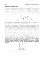
8.5 A Smooth Particle Moving Inside a Vertical Rotating Tube
For a second example illustrating the use of d’Alembert’s principle consider a circular tube
T with radius r rotating with angular speed Ω about a vertical axis as depicted in Figure
8.5.1. Let T contain a smooth particle P with mass m which is free to slide within T. Let
the position of P within T be defined by the angle θ as shown. Let n
r
and n
θ

be radial and
FIGURE 8.4.4
A free-body diagram of the
pendulum mass.
ml
˙˙
sinθθ+=mg 0
Tm=+l
˙
cosθθ
2
mg
˙˙
sinθθ+
()
=g l 0
˙˙
θθ+
()
=g l 0
0593_C08_fm Page 246 Monday, May 6, 2002 2:45 PM
Principles of Dynamics: Newton’s Laws and d’Alembert’s Principle 247
tangential unit vectors, respectively, and let n
2
and n
3
be horizontal and vertical unit vectors,
respectively, fixed in T.
Using the principles of kinematics of Chapter 4 we see that the acceleration of P in an
inertial frame R, in which T is spinning, is (see Eq. (4.10.11)):

(8.5.1)
where P
*
is that point of T that coincides with P. P
*
moves on a horizontal circle with
radius r sinθ. The acceleration of P
*
in R is, then,
(8.5.2)
where n
1
is a unit vector normal to the plane of T.
The velocity and acceleration of P in T are:
(8.5.3)
By substituting from Eqs. (8.5.2) and (8.5.3) into Eq. (8.5.1) the acceleration of P in R
becomes:
(8.5.4)
where
R
ωω
ωω
T
is identified as being Ωn
3
. The unit vectors n
2
and n
3
may be expressed in terms

of n
r
and n
θ
as:
(8.5.5)
By substituting into Eq. (8.5.4) and by carrying out the indicated addition and multipli-
cation,
R
a
P
becomes:
(8.5.6)
FIGURE 8.5.1
A rotating tube with an interior particle P.
n
O
r
n
n
R
n

P(m)
3
2
r
1

n

Ω
θ
θ
RPTPRP R TTP
aaa=+ + ×
*
2 ωωνν
RP
rrann
*
˙
sin sin=− −ΩΩθθ
1
2
2
TP TP
r
rrrνν= =− +
˙

˙˙˙
θθθ
θθ
nann and
2
RP
r
rrr
rn
ann n

nn
=− + −
−+×
˙˙˙˙
sin
sin
˙
θθ θ
θθ
θ
θ
2
1
2
23
24
Ω
ΩΩ
nnn
nnn
2
3
=+
=− +
sin cos
cos sin
θθ
θθ
θ
θ

r
r
RP
r
rr rr
rr
ann
n
=− −
()
+− −
()
+−
()
˙
sin
˙
cos
˙
sin
˙˙
sin cos
ΩΩ Ω
Ω
θθθ θ θ
θθθ
θ
2
1
222

2
0593_C08_fm Page 247 Monday, May 6, 2002 2:45 PM
248 Dynamics of Mechanical Systems
Consider next the forces on P. The inertia force F
*
on P is:
(8.5.7)
The applied forces on P consist of a vertical weight (or gravity) force w given by:
(8.5.8)
and a contact force C given by:
(8.5.9)
(Recall that P is smooth, thus there is no friction or contact force in the n
θ
direction.)
These forces on P are exhibited in the free-body diagram of Figure 8.5.2. Then, from
d’Alembert’s principle, we have:
(8.5.10)
or
(8.5.11)
By substituting from Eq. (8.5.6), and by using Eq. (8.5.5) to express n
3
in terms of n
r
and
n
θ
, the governing equation becomes:
or
(8.5.12)
FIGURE 8.5.2

Free-body diagram of P.
Fa
*
=−m
RP
wn=−mg
3
Cn n=+NN
rr11
CwF++=
*
0
N N mg m
rr
RP
11 3
0nn n a+− − =
N N mg mg mr mr
mr mr mr mr
rr r q
r
11 1
222 2
2
0
nn n n n
nn
+− − + +
()
++

()
+− +
()
=
cos sin
˙
sin
˙
cos
˙
sin
˙˙
sin cos
θθ θθθ
θθθθθ
θ
ΩΩ
ΩΩ
Nmr mr
Nmg mr mr
mr mr mg
rr
11
222
2
2
0
++
()
++ + +

()
+− + −
()
=
˙
sin
˙
cos
cos
˙
sin
˙˙
sin cos sin
ΩΩ
Ω
Ω
θθθ
θθ θ
θθθθ
θ
n
n
n
0593_C08_fm Page 248 Monday, May 6, 2002 2:45 PM
Principles of Dynamics: Newton’s Laws and d’Alembert’s Principle 249
Therefore, the scalar governing equations are:
(8.5.13)
(8.5.14)
(8.5.15)
Equations (8.5.13), (8.5.14), and (8.5.15) are three equations for the unknowns N

1
, N
r
,
and θ. Observe that Eq. (8.5.15) involves only θ. Hence, by solving Eq. (8.5.15) for θ we
can then substitute the result into Eqs. (8.5.13) and (8.5.14) to obtain N
1
and N
r
. Observe
further that if Ω is zero, Eq. (8.5.15) takes the same form as Eq. (8.4.4), the pendulum
equation. We will consider the solution of Eq. (8.5.15) in Chapters 12 and 13.
8.6 Inertia Forces on a Rigid Body
For a more general example of an inertia force system, consider a rigid body B moving
in an inertial frame R as depicted in Figure 8.6.1. Let G be the mass center of B and let P
i
be a typical point of B. Then, from Eq. (4.9.6), the acceleration of P
i
in R may be expressed as:
(8.6.1)
where G is the mass center of B, r
i
is the position vector of P
i
relative to G, αα
αα
is the angular
acceleration of B in R, and ωω
ωω
is the angular velocity of B in R.

Let B be considered to be composed of particles such as the crystals of a sandstone. Let
P
i
be a point of a typical particle having mass m
i
. Then, from Eq. (8.2.5), the inertia force
on the particle is:
(8.6.2)
The inertia forces on B consist of the system of forces made up of the inertia forces on
the particles of B. This system of forces (usually a very large number of forces) may be
represented by an equivalent force system (see Section 6.5) consisting of a single force F
*
FIGURE 8.6.1
A rigid body moving in an inertial
reference frame.
Nmr mr
1
2=− −
˙
sin
˙
cosΩΩθθθ
Nmg mrmr
r
=− − −cos
˙
sinθθ θ
222
Ω
˙˙

sin cos sinθθθ θ−+
()
=Ω
2
0gr
R
P
RG
ii
i
aa r r=+×+××
()
ααωωωω
Fm i
ii
R
P
i
*
=−
()
a nosumon
0593_C08_fm Page 249 Monday, May 6, 2002 2:45 PM
250 Dynamics of Mechanical Systems
passing through an arbitrary point (say G) together with a couple with torque T
*
. Then,
F
*
and T

*
are:
(8.6.3)
and
(8.6.4)
where N is the number of particles of B. Recall that we already examined the summation
in Eqs. (8.6.3) and (8.6.4) in Section 7.12. Specifically, by using the definitions of mass
center and inertia dyadic we found that F
*
and T
*
could be expressed as (see Eqs. (6.9.9),
(7.12.1), and (7.12.8)):
(8.6.5)
and
(8.6.6)
where M is the total mass of B.
Consider the form of the inertia torque: Suppose n
1
, n
2
, and n
3
are mutually perpen-
dicular unit vectors parallel to central principal inertia axes of B. Then, the inertia dyadic
I
B/G
may be expressed as:
(8.6.7)
Let the angular acceleration and angular velocity of B be expressed as:

(8.6.8)
Then, in terms of the α
i
, ω
i
, I
ii
, and the n
i
(i = 1, 2, 3), the inertia torque T
*
may be expressed
as:
(8.6.9)
where the components T
i
(i = 1, 2, 3) are:
(8.6.10)
(8.6.11)
(8.6.12)
FF a
*
*
==
==
∑∑
i
i
R
P

i
N
i
N
m
i
11
TrF ra
*
*
=×=− ×
==
∑∑
i
i
ii
RP
i
N
i
N
m
i
11
Fa
*
=−M
RG
TI I
*

=− ⋅ − × ⋅
()
BG BG
ααωωωω
Innnnnn
BG
II I=++
1111 2222 3333
αα
ωω
=++=
=++=
ααα α
ωωω ω
11 22 33
11 22 33
nnnn
nnnn
ii
ii
and
Tnnnn
*
=++=TTT T
ii11 22 33
TI II
1 1 11 2 3 22 33
=− + −
()
αωω

TI II
2 2 22 3 1 33 11
=− + −
()
αωω
TI II
3 3 33 1 2 11 22
=− + −
()
αωω
0593_C08_fm Page 250 Monday, May 6, 2002 2:45 PM
Principles of Dynamics: Newton’s Laws and d’Alembert’s Principle 251
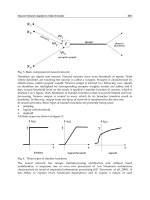
8.7 Projectile Motion
To illustrate the use of Eqs. (8.6.5) and (8.6.6), consider a body thrown into the air as a
projectile as in Figure 8.7.1. Then, the only applied forces on B are due to gravity, which
can be represented by the single weight force W passing through G as:
(8.7.1)
where N
3
is the vertical unit vector shown in Figure 8.7.1. Figure 8.7.2 shows a free-body
diagram of B. Using d’Alembert’s principle, the governing equations of motion of B are,
then,
(8.7.2)
and
(8.7.3)
or
(8.7.4)
and
(8.7.5)
Suppose the acceleration of G is expressed in the form:

(8.7.6)
FIGURE 8.7.1
A body B moving as a projectile.
FIGURE 8.7.2
A free-body diagram of projectile B.
G
W
F*
T*
W =−MgN
3
W +=F
*
0
T
*
= 0
RG
gaN=−
3
TTT
123
0===
RG
xyzaNNN=++
˙˙
˙˙
˙˙
123
0593_C08_fm Page 251 Monday, May 6, 2002 2:45 PM

252 Dynamics of Mechanical Systems
where (x, y, z) are the coordinates of G relative to the X-, Y-, Z-axes system of Figure 8.7.1.
Then, by substituting into Eq. (8.7.4), we obtain the scalar equations:
(8.7.7)
These are differential equations governing the motion of a projectile. They are easy to
solve given suitable initial conditions. For example, suppose that initially (at t = 0) we
have G at the origin O and projected with speed V
O
in the X–Z plane at an angle θ relative
to the X-axis as shown in Figure 8.7.3. Specifically, at t = 0, let x, y, z, , , and be:
(8.7.8)
Then, by integrating, we obtain the solutions of Eq. (8.6.19) in the forms:
(8.7.9)
(8.7.10)
(8.7.11)
By eliminating t between Eqs. (8.7.9) and (8.7.11), we obtain:
(8.7.12)
Equations (8.7.10) and (8.7.12) show that G moves in a plane, on a parabola. That is, a
projectile always has planar motion and its mass center traces out a parabola.
From Eq. (8.7.11), we see that G is on the X-axis (that is, z = 0) when:
(8.7.13)
The corresponding positions on the X-axis are:
(8.7.14)
FIGURE 8.7.3
Projectile movement.
˙˙
,
˙˙
,
˙˙

xyzg===−00
˙
x
˙
y
˙
z
xyz xV y zV
OO
=== = = =00,
˙
cos ,
˙
,
˙
sinθθ
xV t
O
=
()
cosθ
y = 0
zgt V t
O
=− +
()
2
2 sinθ
VzgxV x
OO

22 2 2
2cos sin cosθθθ
()
=−
()
+
()
ttVg
O
==
()
02 sin and θ
xxdVg
O
===
()
02
2
sin cos and θθ
0593_C08_fm Page 252 Monday, May 6, 2002 2:45 PM
Principles of Dynamics: Newton’s Laws and d’Alembert’s Principle 253
where d is the distance from the origin to where G returns again to the horizontal plane,
or to the X-axis (see Figure 8.7.3). For a given V
O
, Eq. (8.7.14) shows that d has a maximum
value when θ is 45°.
Next, consider Eq. (8.7.5). Suppose that the unit vectors n
i
(i = 1, 2, 3) are not only parallel
to principal inertia axes but are also fixed in B. Then, from Eq. (4.6.6), we have:

(8.7.15)
Equation (8.7.5) then takes the form (see Eqs. (8.6.10) to (8.6.12)):
(8.7.16)
(8.7.17)
(8.7.18)
These equations form a system of nonlinear differential equations. A simple solution of
the equations is seen to be:
(8.7.19)
That is, a projectile can rotate with constant speed about a central principal inertia axis.
(We will examine the stability of such rotation in Chapter 13.)
Finally, observe that if a projectile B is rotating about a central principal axis and a point
Q of B is not on the central principal axis, then Q will move on a circle whose center
moves on a parabola. Moreover, a projectile always rotates about its mass center, which
in turn has planar motion on a parabola.
8.8 A Rotating Circular Disk
For another illustration of the effects of inertia forces and inertia torques, consider the
circular disk D with radius r rotating in a vertical plane as depicted in Figure 8.8.1. Let D
be supported by frictionless bearings at its center O.
FIGURE 8.8.1
A rotating circular disk.
αωαωαω
112233
===
˙
,
˙
,
˙
˙
ωωω

123223311
=−
()
III
˙
ωωω
231331122
=−
()
III
˙
ωωω
312112233
=−
()
III
ωωωω
1023
0===,
0593_C08_fm Page 253 Monday, May 6, 2002 2:45 PM
254 Dynamics of Mechanical Systems
Consider two loading conditions on D: First, let D be loaded by a force W applied to
the rim of D as in Figure 8.8.2a. Next, let D be loaded by a weight having mass m attached
by a cable to the rim of D as in Figure 8.8.2b. Let m have the value W/g (that is, the mass
has weight W).
Consider first the loading of Figure 8.8.2a. The force W will cause a clockwise angular
acceleration α
a
as viewed in Figure 8.8.2a. This angular acceleration will in turn induce a
counterclockwise inertia torque component when the equivalent inertia force is passed

through O. A free-body diagram is shown in Figure 8.8.3, where I
O
is the axial moment
of inertia of D, M is the mass of D, and O
x
and O
y
are horizontal and vertical bearing
reaction components. By adding forces horizontally and vertically, by setting the results
equal to zero, and by setting moments about O equal to zero, we obtain:
(8.8.1)
(8.8.2)
and
(8.8.3)
Next, for the loading of Figure 8.8.2b, the weight will create a tension T in the attachment
cable which in turn will induce a clockwise angular acceleration α
b
of D and a resulting
counterclockwise inertia torque. Free-body diagrams for D and the attached weight are
shown in Figure 8.8.4, where the term rα
b
is the magnitude of the acceleration of the
weight. By setting the resultant forces and moments about O equal to zero, we obtain:
(8.8.4)
(8.8.5)
(8.8.6)
(8.8.7)
FIGURE 8.8.2
Two loading conditions on a circular disk.
FIGURE 8.8.3

Free-body diagram of disk in
Figure 8.8.2a.
O
x
= 0
OmgW
y
−−=0
IW
Oa r
α− =0
O
x
= 0
OMgT
y
−−=0
ITr
O
b
α− −0
mr T W
b
α+ − =0
0593_C08_fm Page 254 Monday, May 6, 2002 2:45 PM
Principles of Dynamics: Newton’s Laws and d’Alembert’s Principle 255
By eliminating T from these last two expressions and solving for α
b
, we obtain:
(8.8.8)

From Eq. (8.8.3), α
a
is:
(8.8.9)
By comparing Eqs. (8.8.8) and (8.8.9), we see the effect of the inertia of the weight in
reducing the angular acceleration of the disk.
8.9 The Rod Pendulum
For another illustration of the use of Eqs. (8.6.10), (8.6.11), and (8.6.12), consider a rod of
length ᐉ supported by a frictionless hinge at one end and rotating in a vertical plane as
shown in Figure 8.9.1. Because the rod rotates in a vertical plane about a fixed horizontal
axis, the angular velocity and angular acceleration of the rod are simply:
(8.9.1)
where θ is the inclination angle (see Figure 8.9.1), and n
z
is a unit vector parallel to the
axis of rotation and perpendicular to the unit vectors n
x
, n
y
, n
r
, and n
θ
as shown in
Figure 8.9.1.
FIGURE 8.8.4
Free body diagrams of the disk and
weight for the loading of Figure
8.8.2b.
FIGURE 8.9.1

The rod pendulum.
α
b
O
Wr I mr=+
()
2
α
aO
Wr I=
ωωαα==
˙˙˙
θθnn
zz
and
0593_C08_fm Page 255 Monday, May 6, 2002 2:45 PM
256 Dynamics of Mechanical Systems
The mass center G moves in a circle with radius ᐉ/2. The acceleration of G is:
(8.9.2)
Due to the symmetry of the rod, n
r
, n
θ
, and n
z
are principal unit vectors of inertia (see
Section 7.9). The central inertia dyadic of the rod is:
(8.9.3)
where m is the mass of the rod.
Using Eqs. (8.6.5) and (8.6.6), the inertia force system on the rod is equivalent to a single

force F
*
passing through G together with a couple with torque T
*
, where F
*
and T
*
are:
(8.9.4)
Consider a free-body diagram of the rod as in Figure 8.9.2 where O
x
and O
y
are horizontal
and vertical components of the pin reaction force: using d’Alembert’s principle we can
set the sum of the moments of the forces about the pinned end equal to zero. This sum
leads to:
or
(8.9.5)
Observe that the coefficient of in Eq. (8.9.5), mᐉ
2
/3, may be recognized as I
O
, the
moment of inertia of the rod about O for an axis perpendicular to the rod. That is, from
the parallel axis theorem (see Section 7.6), we have:
FIGURE 8.9.2
Free-body diagram of the rod pendulum.
O

O
mᐉ /2
mg
(1/2)mᐉ
y
x
2
2

θ

θ
mᐉ /2

θ
¨
¨
an n
G
r
=
()
−
()
ll22
2
˙˙ ˙
θθ
θ
Inn

Grr
mmnn=
()
+
()
112 112
22
ll
θθ
FnnT n
**
˙˙ ˙

˙˙
=−
()
+
()
=−
()
mm m
rz
ll l22 112
22
θθ θ
θ
and
mmg mll l l2 2 2 1 12 0
2
()()

+
()
+
()
=
˙˙
sin
˙˙
θθθ
mmgll
2
320
()
+
()
=
˙˙
sinθθ
˙˙
θ
IIm
OG
=+
()
l 2
2
0593_C08_fm Page 256 Monday, May 6, 2002 2:45 PM