Dynamics of Mechanical Systems 2009 Part 8 docx

332 Dynamics of Mechanical Systems
If we multiply the terms of Eq. (10.6.12) by v
G
, the velocity of G in R, we have:
(10.6.14)
Similarly, if we multiply the terms of Eq. (10.6.13) by ωω
ωω
we have:
(10.6.15)
By adding the terms of Eqs. (10.6.14) and (10.6.15), we obtain:
(10.6.16)
From Eqs. (10.4.1), (10.4.2), and (10.4.3) we can recognize the left side of Eq. (10.6.16) as
the derivative of the work W of the force system acting on B. Also, from Eq. (10.5.7) we
recognize the right side of Eq. (10.6.16) as the derivative of the kinetic energy K of B.
Hence, Eq. (10.6.16) takes the form:
(10.6.17)
Then, by integrating, we have:
(10.6.18)
where, as in Eqs. (10.6.5) and (10.6.10), K
2
and K
1
represent the kinetic energy of B at the
beginning and end of the time interval that forces are acting on B.
Equations (10.6.5), (10.6.10), and (10.6.18) are expressions of the principle of work and
kinetic energy for a particle, a set of particles, and a rigid body, respectively. Simply stated,
the work done is equal to the change in kinetic energy.
In the remaining sections of this chapter we will consider several examples illustrating
application of this principle. We will also consider combined application of this principle
with the impulse–momentum principles of Chapter 9.
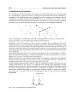
10.7 Elementary Example: A Falling Object

Consider first the simple case of a particle P with mass m released from rest at distance
h above a horizontal surface S as in Figure 10.7.1. The objective is to determine the speed
v of P when it reaches S.
Fv a v v⋅= ⋅=




GGG G
M
d
dt
M
1
2
2
TI I⋅=⋅
()
⋅+ ×⋅
()
[]
⋅= ⋅⋅




ωωααωωωωωωωωωωωωI
d
dt
1

2
0
Fv T v I⋅+⋅=




+⋅⋅




GG
d
dt
M
d
dt
ωωωωωω
1
2
1
2
2
dW
dt
dK
dt
=
WK K K=−=

21
∆
0593_C10_fm Page 332 Monday, May 6, 2002 2:57 PM
Introduction to Energy Methods 333
Because gravity is the only force applied to P and because the path of movement of P
is parallel to the weight force through a distance h, the work done W is simply:
(10.7.1)
Because P is released from rest, its initial kinetic energy is zero. When P reaches S, its
kinetic energy may be expressed as:
(10.7.2)
Then, from the work–energy principle of Eq. (10.6.5), we have:
(10.7.3)
Solving for v, we obtain the familiar result:
(10.7.4)
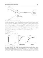
10.8 Elementary Example: The Simple Pendulum
Consider next the simple pendulum depicted in Figure 10.8.1 where the mass m of the
pendulum is concentrated in the bob P which is supported by a pinned, massless rod of
length ᐉ as shown. Let θ measure the inclination of the pendulum to the vertical. Suppose
the pendulum is held in a horizontal position and released from rest. The objective is to
determine the speed v of P as it passes through the equilibrium position θ = 0. If we
consider a free-body diagram of P as in Figure 10.8.2, we see that of the two forces applied
to P the tension of the connecting rod does no work on P because its direction is perpen-
dicular to the movement of P. From Eq. (10.2.18), we see that the work W done by the
weight force is:
(10.8.1)
FIGURE 10.7.1
A particle released from rest in a
gravitational field.
h
S

O
P(m)
W mgh=
Kmv=
1
2
2
W K mgh mv==∆ or
1
2
2
vgh= 2
Wmg= l
0593_C10_fm Page 333 Monday, May 6, 2002 2:57 PM
334 Dynamics of Mechanical Systems
Because the pendulum is released from rest its initial kinetic energy is zero. Its kinetic
energy K as it passes through the equilibrium position may be expressed as:
(10.8.2)
From the work–energy principle of Eq. (10.6.5), we then have:
(10.8.3)
or
(10.8.4)
Observe that this speed is the same as that of an object freely falling through a distance
ᐉ (see Eq. (10.7.4)), even though the direction of the velocity is different.
As a generalization of this example, consider a pendulum released from rest at an angle
θ
i
with the objective of determining the speed of P when it falls to an angle θ
f
, as in Figure

10.8.3. The work
i
W
f
done by gravity as the pendulum falls from θ
i
to θ
f
is:
(10.8.5)
where ∆h is the change in elevation of P as the pendulum falls (see Eq. (10.2.20)).
The kinetic energies K
i
and K
f
of P when θ is θ
i
and θ
f
are:
(10.8.6)
where
i
and
f
are the values of when θ is θ
i
and θ
f
, respectively.

The work–energy principle then leads to:
(10.8.7)
FIGURE 10.8.1
A simple pendulum.
FIGURE 10.8.2
Free body diagram of the pendulum bob.
O
θ
P(m)
ᐉ
T
mg
P
Kmv m==
()
1
2
1
2
2
2
l
˙
θ
W K mg mv m===∆ or ll
1
2
1
2
22

˙
θ
vmg= l
i
ff
i
Wmghmg== −
()
∆ l cos cosθθ
Km Km
ii
ff
=
()
==
()
12 0
1
2
2
2
ll
˙˙
θθand
˙
θ
˙
θ
˙
θ

i
ff
i
WKKK==−∆
0593_C10_fm Page 334 Monday, May 6, 2002 2:57 PM
Introduction to Energy Methods 335
or
(10.8.8)
Solving for
f
we have:
(10.8.9)
The result of Eq. (10.8.9) could also have been obtained by integrating the governing
differential equations of motion obtained in Chapter 8. Recall from Eq. (8.4.4) that for a
simple pendulum the governing equation is:
(10.8.10)
Then, by multiplying both sides of this equation by , we have:
(10.8.11)
Because may be recognized as being (1/2)d
2
/dt, we can integrate the equation and
obtain:
(10.8.12)
Because is zero when θ is θ
i
, the constant is –(g/ᐉ)cosθ
i
. Therefore, we have:
(10.8.13)
When θ is θ

f
, Eqs. (10.8.9) and (10.8.13) are seen to be equivalent.
The work–energy principle may also be used to determine the pendulum rise angle
when the speed at the equilibrium position (θ = 0) is known. Specifically, suppose the
angular speed of the pendulum when θ is zero is
o
. Then, the work W done on the
pendulum as it rises to an angle θ
f
is:
(10.8.14)
FIGURE 10.8.3
A simple pendulum released from
rest and falling through angle θ
i
– θ
f
.
O
P
P
θ
i
f
θ
mg m
f
i
f
llcos cos

˙
θθ θ−
()
=
()
1
2
2
˙
θ
˙
cos cos
/
θθθ
ff
i
g=−
()
2
12
l
˙˙
sinθθ+
()
=g l 0
˙
θ
˙˙˙
sin
˙

θθ θθ+
()
=g l 0
˙
θ
˙˙
θ
˙
θ
12
2
()
−
()
=
˙
cosθθg l constant
˙
θ
˙
cos cosθθθ
2
2=
()
−
()
g
i
l
˙

θ
Wmgh mg
f
==−−
()
∆ l 1 cosθ
0593_C10_fm Page 335 Monday, May 6, 2002 2:57 PM
336 Dynamics of Mechanical Systems
where the negative sign occurs because the upward movement of the pendulum is
opposite to the direction of gravity, producing negative work. The work–energy principle,
then, is:
(10.8.15)
or
(10.8.16)
or
(10.8.17)
If the pendulum is to rise all the way to the vertical equilibrium position (θ = π), we have:
(10.8.18)
If is exactly 4gᐉ, the pendulum will rise to the vertical equilibrium position and come
to rest at that position. If exceeds 4gᐉ, the pendulum will rise to the vertical position
and rotate through it with an angular speed given by Eq. (10.8.18) (sometimes called the
rotating pendulum).
10.9 Elementary Example — A Mass–Spring System
For a third fundamental example, consider the mass–spring system depicted in Figure
10.9.1. It consists of a block B with mass m and a linear spring, with modulus k, moving
without friction or damping in a horizontal direction. Let x measure the displacement of
B away from equilibrium.
Suppose B is displaced to the right (positive x displacement with the spring in tension)
a distance δ away from equilibrium. Let B be released from rest in this position. Questions
arising then are what is the speed v of B as it returns to the equilibrium position (x = 0),

and how far to the left of the equilibrium position does B go?
FIGURE 10.9.1
Ideal mass–spring system.
00
WKKK
ff
==−∆
−−
()
=
()
()
−
()
()
mg m m
ff
lll112 12
2
0
2
cos
˙˙
θθ θ
˙˙
cosθθ θ
ff
g
2
0

2
21=− −
()
l
˙˙
θθ
f
g
2
0
2
4=−l
˙
θ
0
2
˙
θ
0
2
m
x
B
k
0593_C10_fm Page 336 Monday, May 6, 2002 2:57 PM
Introduction to Energy Methods 337
To answer these questions using the work–energy principle, recall from Eq. (10.2.22)
that when a linear spring is stretched (or compressed) a distance δ, the corresponding
work W done by the stretching (or compressing) force is (1/2)kδ
2

. Because the force exerted
on the spring is equal, but oppositely directed, to the force exerted on B, the work done
on B as the spring is relaxed is also (1/2)kδ
2
. (That is, the work on B is positive because
the force of the spring on B is in the same direction as the movement of B.)
Because B is released from rest, its initial kinetic energy is zero. The kinetic energy at
the equilibrium position is:
(10.9.1)
Then, from the work–energy principle, we have:
(10.9.2)
or
(10.9.3)
where the minus sign is selected because B is moving to the left.
Next, as B continues to move to the left past the equilibrium position, the spring force
will be directed opposite to the movement of B. Therefore, the work W done on B as B
moves to the left a distance d from the equilibrium position is:
(10.9.4)
When B moves to its leftmost position, its kinetic energy is zero. From Eqs. (10.9.1) and
(10.9.2), the kinetic energy of B at the equilibrium position is:
(10.9.5)
The work–energy principle then produces:
(10.9.6)
or
(10.9.7)
That is, the block moves to the left by precisely the same amount as it was originally
displaced to the right.
The usual explanation of this phenomenon is that when the spring is stretched (or
compressed) the work done by the stretching (or compressing) force stores energy (potential
energy) in the spring. This stored energy in the spring is derived from the kinetic energy

of the block. Then, as the spring is relaxing, its potential energy is transferred back to
kinetic energy of the block. There is thus a periodic transfer of energy between the spring
Kmv mx=
()
=
()
12 12
22
˙
WK k mv=
()
=
()
−∆ or 12 12 0
22
δ
vx km==
˙
δ
Wkd=−
()
12
2
Kmv k=
()
=
()
12 12
22
δ

W K kd k=−
()
=−
()
∆ or 1 2 0 1 2
22
δ
d =δ
0593_C10_fm Page 337 Monday, May 6, 2002 2:57 PM
338 Dynamics of Mechanical Systems
and the block, with the sum of the potential energy of the spring and the kinetic energy
of the block being constant. (We will discuss potential energy in the next chapter.)
As another example of work–energy transfer, consider the mass–spring system arranged
vertically as in Figure 10.9.2. Suppose B is held in a position where the spring is
unstretched. If B is then released from rest from this position, it will fall and stretch the
spring and eventually come to rest at an extreme downward position. Questions arising
then include how far does B fall and what is the spring force when B reaches this maximum
downward displacement? To answer these questions, consider that as B falls, the weight
(or gravity) force on B is in the direction of the movement of B, whereas the spring force
on B is opposite to the movement of B. Because B is at rest at both the beginning and the
end of the movement, there is no change in the kinetic energy of B. The net work on B is
then zero. That is,
(10.9.8)
where d is the distance B moves downward. By solving for d we obtain:
(10.9.9)
The spring force in this extended position is, then,
(10.9.10)
The result of Eq. (10.9.10) shows that a suddenly applied weight load on a spring creates
a force twice that of the weight. This means that if a weight is suddenly placed on a
machine or structure the force generated is twice that required to support the weight in

a static equilibrium configuration.
10.10 Skidding Vehicle Speeds: Accident Reconstruction Analysis
The work–energy principle is especially useful in determining speeds of accident vehi-
cles by using measurements of skid-mark data. Indeed, the work–energy principle
together with the conservation of momentum principles are the primary methods used
by accident reconstructionists when attempting to determine vehicle speeds at various
stages of an accident.
FIGURE 10.9.2
A vertical mass–spring system.
k
Y
m
B
W mgd kd== −
()
012
2
dmgk= 2
Fkd mg==2
0593_C10_fm Page 338 Monday, May 6, 2002 2:57 PM
Introduction to Energy Methods 339
To illustrate the procedure, suppose an automobile leaves skid marks from all four
wheels in coming to an emergency stop. Given the length d of the skid marks, the objective
is to determine the vehicle speed when the marks first began.
Skid marks are created by abrading and degrading tires sliding on a roadway surface.
The tire degradation is due to friction forces and heat abrading the rubber. The friction
forces are proportional to the normal (perpendicular to the roadway surface) forces on
the tires and to the coefficient of friction µ. The friction coefficient, ranging in value from
0 to 1.0, is a measure of the relative slipperiness between the tires and the roadway
pavement. If F and N are equivalent friction and normal forces (see Section 6.5), they are

related by the expression:
(10.10.1)
If an automobile is sliding on a flat, level (horizontal) roadway, a free-body diagram of
the vehicle shows that the normal force N is equal to the vehicle weight w. Then, as the
vehicle slides a distance d, the work W done by the friction force (acting opposite to the
direction of the sliding) is:
(10.10.2)
where m is the mass of the automobile.
Let v be the desired speed of the automobile when the skid marks first appear. Then,
the kinetic energy K
i
of the vehicle at that point is:
(10.10.3)
Because the kinetic energy K
f
at the end of the skid marks is zero (the vehicle is then
stopped), the work energy principle produces:
(10.10.4)
or
(10.10.5)
Observe that the calculated speed is independent of the automobile mass.
To illustrate how the work–energy principle may be used in conjunction with the
momentum conservation principles, suppose an automobile with mass m
1
slides a distance
d
1
before colliding with a stopped automobile having mass m
2
. Suppose further that the

two vehicles then slide together (a plastic collision) for a distance d
2
before coming to rest.
The questions arising then are what were the speeds of the vehicles just before and just
after impact and what was the speed of the first vehicle when it first began to slide?
To answer these questions, consider first from Eq. (10.10.5) that the speed v
a
of the
vehicles just after impact is:
(10.10.6)
FN=µ
W Fd Nd wd mgd=− =− =− =−µµµ
Kmv
i
=
()
12
2
W K K K mgd mv
f
i
==− − =−
()
∆ or µ 012
2
vgd= 2µ
vgd
a
= 2
2

µ
0593_C10_fm Page 339 Monday, May 6, 2002 2:57 PM
340 Dynamics of Mechanical Systems
Next, during impact, the momentum is conserved. That is,
(10.10.7)
where v
b
is the speed of the first vehicle just before impact (see Eq. (9.7.1)).
From Eq. (10.10.2), the work W done by friction forces on the first vehicle as it slides a
distance d
1
before the collision is:
(10.10.8)
If v
0
is the speed of the first vehicle when skidding begins, the change in kinetic energy
of the vehicle from the beginning of skidding until the collision is:
(10.10.9)
The work–energy principle then gives:
(10.10.10)
Finally, using Eqs. (10.10.6) and (10.10.7), we can solve Eq. (10.10.10) for :
(10.10.11)
Observe from Eq. (10.10.7) that the speed v
a
of the first vehicle just after the collision
with the second vehicle is reduced by the factor [m
1
/(m
1
+ m

2
)]. That is, the change in
speed ∆v is:
(10.10.12)
Observe further that because the velocity changes during the impact the kinetic energy
also changes. That is, even though the momentum is conserved, the kinetic energy is not
conserved. Indeed, the change in kinetic energy ∆K just before and just after the impact is:
(10.10.13)
In actual accidents, the vehicles do not usually leave uniform skid marks from all four
wheels. Also, collisions are not usually perfectly plastic nor do the vehicles always move
in a straight line on a level surface. However, with minor modifications, the work–energy
and momentum conservation principles may still be used to obtain reasonable estimates
of vehicle speeds at various stages of an accident. The details of these modifications and
the corresponding application of the principles are beyond the scope of this text; the reader
is referred to the references for further information.
mv m m v
b
a112
=+
()
Wmgd=−µ
11
∆Kmv mv
b
=
()
−
()
12 12
1

2
10
2
WK mgd mv mv
b
=−=
()
−
()
∆ or µ
11 1
2
10
2
12 12
v
0
2
v v gd m m v gd
m m gd gd
b
a0
22
121
2
2
1
21
2
21

21 2
122
=+ =+
()
[]
+
=+
()
[]
+
µµ
µµ
∆vv v m m mv
a
bb
=−=− +
()
[]
212
∆Kmv mv m
mmmm
mm
v
a
bb
=
()
−
()
=−

()
++
+
()








12 12 12
22
1
2
1
2
1
1
2
12 3
2
12
2
2
0593_C10_fm Page 340 Monday, May 6, 2002 2:57 PM
Introduction to Energy Methods 341
10.11 A Wheel Rolling Over a Step
For a second example illustrating the tandem use of the work–energy principle and the

conservation of momentum principle, consider again the case of the wheel rolling over a
step as in Figure 10.11.1 (recall that we considered this problem in Section 9.9). Let the
wheel W have a radius r, mass m, and axial moment of inertia I. Suppose we are interested
in knowing the speed v of the wheel center required for the wheel to roll over the step.
Recall in Section 9.9 that when the wheel encounters the step its angular momentum
about the corner (or nose) O of the step is conserved. By using the conservation of angular
momentum principle we found that the angular speed of W just after impact is (see
Eq. (9.9.8)):
(10.11.1)
where ω is the angular speed of W before impact and h is the height of the step.
After impact, W rotates about the nose O of the step. For W to roll over the step it must
have enough kinetic energy after impact to overcome the negative work of gravity as it
rises up over the step. The work W
g
of gravity as W rolls completely up the step is:
(10.11.2)
If W just rolls over the step (that is, if W expends all its kinetic energy after impact in
rolling over the step), it will come to rest at the top of the step and its kinetic energy K
f
at that point will be zero. The kinetic energy K
i
just after impact is:
(10.11.3)
The work–energy principle then leads to:
(10.11.4)
Solving we have:
(10.11.5)
Hence, from Eq. (10.11.1), the speed v of W just before impact for step rollover is:
FIGURE 10.11.1
Wheel rolling over a step.

W
ω
h
n
r
O
ˆ
ω
ˆ
/ωω=+ −
()
[]
+
()
{}
Imrrh Imr
2
W mgh
g
=−
K I mr I mr
i
=
()
+
()
=
()
+
()

12 12 12
222 22
ˆˆ ˆ
ωω ω
W K K mgh I mr
g
f
i
=− − =−
()
+
()
or 0 1 2
22
ˆ
ω
ˆ
ω
ˆ
/
/
ω= +
()
[]
2
2
12
mgh I mr
0593_C10_fm Page 341 Monday, May 6, 2002 2:57 PM
342 Dynamics of Mechanical Systems

(10.11.6)
Suppose that W is a uniform circular disk with I then being (1/2)mr
2
. In this case, v
becomes:
(10.11.7)
Observe that the disk could (at least, theoretically) roll over a step whose height h is greater
than r. From a practical perspective, however, the disk will only encounter the nose of the
step if h is less than r.
Observe also that, as with the colliding vehicles, the energy is not conserved when the
wheel impacts the step. From Eq. (10.11.1), the energy loss L is seen to be:
(10.11.8)
For a uniform circular disk, this becomes:
(10.11.9)
10.12 The Spinning Diagonally Supported Square Plate
For a third example of combined application of the work–energy and momentum conser-
vation principles, consider again the spinning square plate supported by a thin wire along
a diagonal as in Figure 10.12.1 (recall that we studied this problem in Section 9.12). As
before, let the plate have side length a, mass m, and initial angular speed Ω. Let the plate
be arrested along an edge so that it rotates about that edge as in Figure 10.12.2.
FIGURE 10.12.1
Suspended spinning square plate.
FIGURE 10.12.2
Arrested plate spinning about an edge.
vr r
I mr mgh
Imrrh
==
+
()

()
[]
+−
()
ω
2
12
2
/
vr gh rh=
()
−
[]
332/
L I mr I mr
Imrh m r h m r h
Imr
=
()
+
()
−
()
−
()
=−
()
+−
+







12 12 12 12
12
22
222222
23 22 2
2
ˆˆ
ωωωω
Lmhrh=− −
()
[]
3
Q
a
0
Ω
Q
O

Ω
0593_C10_fm Page 342 Monday, May 6, 2002 2:57 PM
Introduction to Energy Methods 343
Recall that in Section 9.12 we discovered through the conservation of angular momen-
tum principle that the post-seizure rotation speed is related to the pre-seizure speed Ω
by the expression:

(10.12.1)
In view of the result of Eq. (10.12.1), a question that may be posed is what should the
pre-seizure speed be so that after seizure the plate rotates through exactly 180°, coming
to rest in the upward configuration shown in Figure 10.12.3?
We can answer this question using the work–energy principle. Because gravity is the
only force doing work on the plate, the work W is simply the plate weight multiplied by
the mass center elevation change (see Figure 10.12.4):
(10.12.2)
where the negative sign occurs because the mass center elevation movement is opposite
to the direction of gravity.
The final kinetic energy K
f
is zero because the plate comes to rest. The initial kinetic
energy K
i
just after the plate edge is seized, is:
(10.12.3)
The work–energy principle then produces:
(10.12.4)
Solving for , we obtain:
(10.12.5)
Then, from Eq. (10.12.1), Ω, the pre-seizure angular speed, is:
(10.12.6)
FIGURE 10.12.3
Upward resting configuration of the plate.
FIGURE 10.12.4
Plate mass center elevation change.
Q
O
Q

O
h = a 2 /2
a
G
G
ˆ
Ω
ˆ
/ΩΩ=
()
28
W mgh mga=− =− 22/
Kma mama
i
=
()()
[]
+
()( )
[]
=1 2 2 1 2 1 12 6
2
22 2 2
ˆˆˆ
ΩΩΩ
W K K mga ma
f
i
=− − =−or 2 2 0 6
22

/
ˆ
Ω
ˆ
Ω
ˆ
/
Ω=
[]
32
12
ga
ΩΩ=
()
=
[]
8 2 96 2
12
ˆ
/
ga
0593_C10_fm Page 343 Monday, May 6, 2002 2:57 PM
344 Dynamics of Mechanical Systems
10.13 Closure
The work–energy principle is probably the most widely used of all the principles of
dynamics. The primary advantage of the work–energy principle is that it only requires
knowledge of velocities and not accelerations. Also, calculation of the work done is often
accomplished by inspection of the system configuration.
The major disadvantage of the work–energy principle is that only a single equation is
obtained. Hence, if there are several unknowns with a given mechanical system, at most

one of these can be obtained using the work–energy principle. This in turn means that
the principle is most advantageous for relatively simple mechanical systems. However,
the utility of the principle may often be enhanced by using it in tandem with other
dynamics principles — particularly impulse–momentum principles.
In the next two chapters we will consider more general energy methods. We will consider
the procedures of generalized dynamics, Lagrange’s equations, and Kane’s equations.
These procedures, while not as simple as those of the work–energy principle, have the
advantage of still being computationally efficient and of producing the same number of
equations as there are degrees of freedom of a system.
References (Accident Reconstruction)
10.1. Baker, J. S., Traffic Accident Investigation Manual, The Traffic Institute, Northwestern University,
Evanston, IL, 1975.
10.2. Backaitis, S. H., Ed., Reconstruction of Motor Vehicle Accidents: A Technical Compendium, Publi-
cation PT-34, Society of Automotive Engineers (SAE), Warrendale, PA, 1989.
10.3. Platt, F. N., The Traffic Accident Handbook, Hanrow Press, Columbia, MD, 1983.
10.4. Moffatt, E. A., and Moffatt, C. A., Eds., Highway Collision Reconstruction, American Society of
Mechanical Engineers, New York, 1980.
10.5. Gardner, J. D., and Moffatt, E. A., Eds., Highway Truck Collision Analysis, American Society of
Mechanical Engineers, New York, 1982.
10.6. Adler, U., Ed., Automotive Handbook, Robert Bosch, Stuttgart, Germany, 1986.
10.7. Collins, J. C., Accident Reconstruction, Charles C Thomas, Springfield, IL, 1979.
10.8. Limpert, R., Motor Vehicle Accident Reconstruction and Cause Analysis, The Michie Company,
Low Publishers, Charlottesville, VA, 1978.
10.9. Noon, R., Introduction to Forensic Engineering, CRC Press, Boca Raton, FL, 1992.
Problems
Sections 10.2 and 10.3 Work
P10.2.1: A particle P moves on a curve C defined by the parametric equations:
xt yt zt== =,,
23
0593_C10_fm Page 344 Monday, May 6, 2002 2:57 PM

Introduction to Energy Methods 345
where x, y, and z are coordinates, measured in meters, relative to an X, Y, Z Cartesian
system. Acting on P is a force F given by:
where F is measured in Newtons, and n
x
, n
y
, and n
z
are unit vectors parallel to the X-, Y-,
and Z-axes. Compute the work done by F in moving P from (0, 0, 0) to (2, 4, 8).
P10.2.2: The magnitude and direction of a force F acting on a particle P depend upon the
coordinate position (x, y, z) of F (and P) in an X, Y, Z coordinate space as:
where n
x
, n
y
, and n
z
are unit vectors parallel to X, Y, and Z. Suppose P moves from the
origin O to a point C (1, 2, 3) along two different paths as in Figure P10.2.2: (1) along the
line segment OC, and (2) along the rectangular segments OA, AB, BC. Calculate the work
done by F on P in each case. (Assume that the coordinates are measured in meters.)
P10.2.3: See Problem P10.2.2. Suppose a force F acting on a particle P depends upon the
position of F (and P) in an X, Y, Z space as:
Show that the work done by F on P as P moves from P
1
(x
1
, y

1
, z
1
) to P
2
(x
2
, y
2
, z
2
) is simply
φ (x
2
, y
2
, z
2
) – φ (x
1
, y
1
, z
1
). Comment: When a force F can be represented in the form F =
∇φ, F is said to be conservative.
P10.2.4: See Problems P10.2.2 and P10.2.3. Show that the force F of Problem P10.2.2 is
conservative. Determine the function φ. Using the result of Problem P10.2.3, check the
result of P10.2.2.
P10.2.5: A horizontal force F pushes a 50-lb cart C up a hill H which is modeled as a

sinusoidal curve with amplitude of 7 ft and half-period of 27 ft as shown in Figure P10.2.5.
Assuming that there is no frictional resistance between C and H and that F remains directed
horizontally, find the work done by F.
FIGURE P10.2.2
A particle P moving from O to C along
two different paths.
Fn n n=−+468
xyz
Fn n n=++222
22 2 2 22
xy z x yz x y z N
xyz
P
P
A
C(1,2,3)
B
Z
Y
X
n
n
n
O
z
y
x
Fnnn=∇
=
∂

∂
+
∂
∂
+
∂
∂
φ
φφφ
D
xyz
xyz
0593_C10_fm Page 345 Monday, May 6, 2002 2:57 PM
346 Dynamics of Mechanical Systems
P10.2.6: A force pushes a block B along a smooth horizontal slot from a position O to a
position Q as in Figure P10.2.6. The movement of B is resisted by a linear spring with a
natural (unstretched) length of 6 in. and modulus 12 lb/in. Determine the work done by F.
P10.2.7: Repeat Problem P10.2.6 if the natural length of the spring is 4 in.
P10.2.8: A motorist, in making a turn with a 15-in diameter steering wheel, exerts a force
of 8 lb with each hand tangent to the wheel as in Figure P10.2.8. If the wheel is turned
through an angle of 150°, determine the work done by the motorist.
Section 10.4 Power
P10.4.1: An automobile with a 110-hp engine is traveling at 35 mph. If there are no frictional
losses in the transmission or drive train, what is the tractive force exerted by the drive
wheels?
P10.4.2: See Problem P10.4.1. Suppose the automobile of Problem P10.4.1 has 26-in
diameter drive wheels, a transmission gear ratio of 8 to 1, and a drive axle gear ratio of
4.5 to 1. What is the engine speed (in rpm)? What is the torque (in ft⋅lb) of the engine
crank shaft?
FIGURE P10.2.5

A force F pushing a cart up a hill.
FIGURE P10.2.6
A block sliding in a slot.
FIGURE P10.2.8
Forces on a steering wheel.
7 ft
27 ft
F
H
C
6 in.
k = 12 lb/in.
B B
F
O
Q
8 in.
8 lb
8 lb
15 in. diameter
0593_C10_fm Page 346 Monday, May 6, 2002 2:57 PM
Introduction to Energy Methods 347
Section 10.5 Kinetic Energy
P10.5.1: An 2800-lb automobile starting from a stop accelerates at the rate of 3 mph per
second. Find the kinetic energy of the vehicle after it has traveled 100 yards.
P10.5.2: A double pendulum consists of two particles P
1
and P
2
having masses m

1
and m
2
supported by light cables with lengths ᐉ
1
and ᐉ
2
, making angles θ
1
and θ
2
with the vertical
as in Figure P10.5.2. Find an expression for the kinetic energy of this system. Express the
results in terms of m
1
, m
2
, ᐉ
1
, ᐉ
2
, θ
1
, θ
2
,
1
, and
2
.

P10.5.3: Determine the kinetic energy of the rod pendulum of Figure P10.5.3. Let the rod
have length ᐉ and mass m. Express the result in terms of m, ᐉ, θ, and .
P10.5.4: See Problem 10.5.3. Consider the double rod pendulum as in Figure 10.5.4. Let
each rod have length ᐉ and mass m. Determine the kinetic energy of the system. Express
the results in terms of m, ᐉ, θ
1
, θ
2
,
1
, and
2
.
P10.5.5: See Problems P10.5.3 and P10.5.4. Extend the results of Problems P10.5.3 and
P10.5.4 to the triple-rod pendulum of Figure P10.5.5.
P10.5.6: An automobile with 25-in diameter wheels is traveling at 30 mph when the
operator suddenly swerves to the left, causing the vehicle to spin out and rotate at the
rate of 180°/sec. If the wheels each weigh 62 lb and if their axial and diametral radii of
FIGURE P10.5.2
A double pendulum.
FIGURE P10.5.3
A rod pendulum.
FIGURE P10.5.4
Double-rod pendulum.
˙
θ
˙
θ
θ
ᐉ

P (m )
P (m )
1
1
1 1
2
2
2 2
θ
˙
θ
θ
ᐉ
G
˙
θ
˙
θ
θ
1
2
θ
0593_C10_fm Page 347 Monday, May 6, 2002 2:57 PM
348 Dynamics of Mechanical Systems
gyration are 10 and 7 in., respectively, determine the kinetic energy of one of the rear
wheels for the spinning vehicle.
Sections 10.6 to 10.9: Work–Energy Principles and Applications
P10.6.1: A ball is thrown vertically upward with a speed of 12 m/sec. Determine the
maximum height h reached by the ball.

P10.6.2: An object is dropped from a window which is 45 ft above the ground. What is
the speed of the object when it strikes the ground?
P10.6.3: See Problem P10.6.1. What is the speed of the ball when it is 3 m above the thrower.
P10.6.4: A water faucet is dripping slowly. When a drop has fallen 1 ft, a second drop
appears. What are the speeds of the drops when the first drop has fallen 3 ft? What is the
separation between the drops at that time?
P10.6.5: A simple pendulum consists of a light string of length 3 ft and a concentrated
mass P weighing 5 lb at the end as in Figure P10.6.5. Suppose the pendulum is displaced
through an angle θ of 60° and released from rest. What is the speed of P when θ is (a) 45°,
(b) 30°, and (c) 0°?
P10.6.6: See Problem P10.6.5. Suppose P has a speed of 7.5 ft/sec when θ is 0. What is the
maximum angle reached by P?
P10.6.7: See Problems 10.6.5 and P10.6.6. What is the minimum speed v of P when θ is 0
so that the pendulum will make a complete loop without the string becoming slack even
in the topmost position (θ = 180°)?
P10.6.8: Repeat Problems P10.6.5 to 10.6.7 if the mass of P is 10 lb instead of 5 lb.
P10.6.9: Repeat Problems P10.6.5 to 10.6.7 if the length ᐉ of the pendulum is 4 ft.
FIGURE P10.5.5
Triple-rod pendulum.
FIGURE P10.6.5
A simple pendulum.
θ
1
2
3
θ
θ
θ
ᐉ
O

(3 ft)
P (5 lb)
0593_C10_fm Page 348 Monday, May 6, 2002 2:57 PM
Introduction to Energy Methods 349
P10.6.10: Repeat Problems P10.6.5 and P10.6.6 if the simple pendulum of Figure P10.6.5
is replaced by a rod pendulum of length 3 ft and weight 5 lb as in Figure P10.6.10, with
P being the end point of the rod.
P10.6.11: A block B with mass m is attached to a vertical linear spring with modulus k as
in Figure P10.6.11. Suppose B is held in a position where the spring is neither stretched
nor compressed and is then released from rest. Find:
a. The maximum downward displacement of B
b. The maximum force in the spring
c. The maximum speed of B
d. The position where the maximum speed of B occurs
P10.6.12: Solve Problem P10.6.11 for k = 7 lb/in. and m = 0.25 slug.
P10.6.13: Solve Problem P10.6.11 for k = 12 N/cm and m = 2 kg.
P10.6.14: A 5-lb block B sliding in a smooth vertical slot is attached to a linear spring with
modulus k of 4 lb/in. as in Figure P10.6.14. Let the natural length
ᐉ of the spring be 8 in.
Let the displacement y of B be measured downward from O, opposite the spring anchor
Q as shown. Find the speed of B when (a) y = 0, and (b) y = 5 in.
P10.6.15: Solve Problem P10.6.14 if the natural length of the spring is 6 in.
P10.6.16: A 10-kg block B is placed at the top of an incline which has a smooth surface as
represented in Figure P10.6.16. If B is released from rest and slides down the incline, what
will its speed be when it reaches the bottom of the incline?
FIGURE P10.6.10
A rod pendulum.
FIGURE P10.6.11
A vertical mass–spring
system.

FIGURE P10.6.14
A spring connected block in a smooth
vertical slot.
θ
ᐉ
O
(3 ft)
P
k
B(m)
6 in.
O
y
8 in.
Q
k = 4 lb/in.
B (5 lb)
0593_C10_fm Page 349 Monday, May 6, 2002 2:57 PM
350 Dynamics of Mechanical Systems
P10.6.17: See Problem P10.6.16. A 10-kg circular disk D with 0.25-m diameter is placed at
the top of an incline that has a perfectly rough surface as represented in Figure P10.6.17.
If D is released from rest and rolls down the incline, what will be the speed of the center
O of D when it reaches the bottom of the incline? Compare the result with that of Problem
P10.6.16.
P10.6.18: A solid half-cylinder C, with radius r and mass m, is placed on a horizontal
surface S and held with its flat side vertical as represented in Figure P10.6.18. Let C be
released from rest and let S be perfectly rough so that C rolls on S. Determine the angular
speed of C when its mass center G is in the lowest most position.
P10.6.19: Repeat Problem P10.6.18 if S is smooth instead of rough.
P10.6.20: A 7-kg, 1.5-m-long rod AB has its end pinned to light blocks that are free to move

in frictionless horizontal and vertical slots as represented in Figure P10.6.20. If the pins
are also frictionless, and if AB is released from rest in the position shown, determine the
speed of the mass center G and the angular speed of AB when AB falls to a horizontal
position and when AB has fallen to a vertical position. Assume that the guide blocks at
A and B remain in their vertical and horizontal slots, respectively, throughout the motion.
P10.6.21: Repeat Problem P10.6.20 if the guide blocks at A and B are no longer light but
instead have masses of 1 kg each.
FIGURE P10.6.16
A block sliding down a smooth inclined
surface.
FIGURE P10.6.17
A circular disk D rolling down an incline plane.
FIGURE P10.6.18
A half-cylinder (end view) on a
horizontal surface.
FIGURE P10.6.20
A rod with ends moving in
frictionless guide slots.
4 m
B
30°
smooth
4 m
30°
D
O
Perfectly
rough
G
C

S
Perfectly
rough
A
B
G
1.5 m
0593_C10_fm Page 350 Monday, May 6, 2002 2:57 PM
Introduction to Energy Methods 351
P10.6.22: A 300-lb flywheel with radius of gyration of 15 in. is rotating at 3000 rpm. A
bearing failure causes a small friction moment of 2 ft⋅lb which in turn causes the flywheel
to slow and eventually stop. How many turns does the flywheel make before coming to
a stop?
Section 10.10 Motor Vehicle Accident Reconstruction
P10.10.1: All four wheels of a car leave 75-ft-long skid marks in coming to a stop on a
level roadway. If the coefficient of friction between the tires and the road surface is 0.75,
determine the speed of the car at the beginning of the skid marks.
P10.10.2: The front wheels of a car leave 70 ft of skid marks and its rear wheels leave 50
ft of skid marks in coming to a stop on a level roadway. If the coefficient of friction between
the tires and the roadway is 0.80, and if 60% of the vehicle weight is on the front wheels,
determine the speed of the car at the beginning of the skid marks.
P10.10.3: A car slides to a stop leaving skid marks of length s (measured in feet) on a level
roadway. If the coefficient of friction between the tires and the roadway is µ, show that
the speed v (in miles per hour) of the car at the beginning of the skid marks is given by
the simple expression:
P10.10.4: See Problem P10.10.3. Suppose that the roadway, instead of being level, has a
slight down slope in the direction of travel as represented in Figure P10.10.4. If the down
slope angle is θ (measured in radians) as shown, show that the speed formula of Problem
P10.10.3 should be modified to:
P10.10.5: An automobile leaves 50 ft of skid marks before striking a pole at 20 mph. Find

the speed of the vehicle at the beginning of the skid marks if the roadway is level and if
the coefficient of friction between the tires and the roadway is 0.65. Assume the vehicle
stops upon hitting the pole.
P10.10.6: A pickup truck leaves 30 ft of skid marks before colliding with the rear of a
stopped automobile. Following the collision, the two vehicles slide together (a plastic
collision) for 25 ft. Let the coefficient of friction between the pickup truck tires and the
roadway be 0.7; after the collision, for the sliding vehicles together, let the coefficient of
friction with the roadway be 0.5. Let the weights of the pickup truck and automobile be
3500 lb and 2800 lb, respectively. Find the speed of the pickup truck at the beginning of
the skid marks.
P10.10.7: Repeat Problem P10.10.6 if just before collision, instead of being stopped, the
automobile is moving at 10 mph in the same direction as the pickup truck.
FIGURE P10.10.4
An automobile A skidding to a stop on
a downslope.
vs= 30µ
vs=−
()
30 µθ
A
θ
v
0593_C10_fm Page 351 Monday, May 6, 2002 2:57 PM
352 Dynamics of Mechanical Systems
P10.10.8: Repeat Problem P10.10.6 if just before collision, instead of being stopped, the
automobile is moving toward the pickup truck at 10 mph (that is, a head-on collision).
Sections 10.11 and 10.12 Work, Energy, and Impact
P10.11.1: A 60-gauge bullet is fired into a 20-kg block suspended by a 7-m cable as depicted
in Figure P10.11.1. The impact causes the block pendulum to swing through an angle of
15°. Determine the speed v of the bullet.

P10.11.2: A 14-in. diameter wheel W
1
is rotating at 350 rpm when it is brought into contact
with a 10-in diameter wheel W
2
, which is initially at rest, as represented in Figure P10.11.2.
After the wheels come into contact, they roll together without slipping. Although W
1
is free
to rotate, with negligible friction, W
2
is subjected to a frictional moment of 2 ft⋅lb in its
bearings. Let the weights of W
1
and W
2
be 28 lb and 20 lb, respectively. Let the radii of
gyration of W
1
and W
2
be 5 in. and 3.5 in., respectively. Determine the number of revolutions
N
1
and N
2
turned by each wheel after the meshing contact until they come to rest.
P10.11.3: A 1-m rod B with a mass of 1 kg is hanging
vertically and supported by a frictionless pin at O as
in Figure P10.11.3. A particle P with a mass of 0.25

kg moving horizontally with speed v collides with
the rod as also indicated in Figure P10.11.3. If the
collision is perfectly plastic (with coefficient of resti-
tution e = 0), determine v so that B completes exactly
one half of a revolution and then comes to rest in a
vertically up position. Let the point of impact x be
(a) 0.5 m; (b) 0.667 m; and (c) 1.0 m.
P10.11.4: Repeat Problem P10.11.3 for a perfectly
elastic collision (coefficient of restitution e = 1).
FIGURE P10.11.1
A bullet fired into a block.
FIGURE P10.11.2
Meshing wheels.
60 g
v
7 m
20 kg
W (20 lb)
5 in.
Initially at rest
2
7 in.
300 rpm
1
W (28 lb)
FIGURE P10.11.3
A particle P colliding with a vertical pin
supported rod initially at rest.
P
x

O
B
1 m
v
0593_C10_fm Page 352 Monday, May 6, 2002 2:57 PM

353

11

Generalized Dynamics: Kinematics and Kinetics

11.1 Introduction

Recall in the analysis of elementary statics problems we discover, after gaining e

x

perience,
that by making insightful choices about force directions and moment points, we can greatly
simplify the analysis. Indeed, with sufficient insight, we discover that we can often obtain
precisely the same number of equations as there are unknowns in the problem statement.
Moreover, these equations are often uncoupled, thus producing answers with little further
analysis.
In Chapter 10, we found that the work–energy principle, like clever statics solution
procedures, can often produce simple and direct solutions to dynamics problems. We also
found, however, that while the work–energy principle is simple and direct, it is also quite
restricted in its range of application. The work–energy principle leads to a single scalar
equation, thus enabling the determination of a single unknown. Hence, if two or more
unknowns are to be found, the work–energy principle is inadequate and is restricted to

relatively simple problems.
The objective of

generalized dynamics

is to extend the relatively simple analysis of the
work–energy principle to complex dynamics problems having a number of unknowns.
The intention is to equip the analyst with the means of determining unknowns with a
minimal effort — as with insightful solutions of statics problems.
In this chapter, we will introduce and discuss the elementary procedures of generalized
dynamics. These include the concepts of generalized coordinates, partial velocities and
partial angular velocities, generalized forces, and potential energy. In Chapter 12, we will
use these concepts to obtain equations of motion using Kane’s equations and Lagrange’s
equations.

11.2 Coordinates, Constraints, and Degrees of Freedom

In the conte

x

t of generalized dynamics, a

coordinate

(or

generalized coordinate

) is a parameter

used to define the configuration of a mechanical system. Consider, for example, a particle

P

moving on a straight line

L

as in Figure 11.2.1. Let

x

locate

P

relative to a fixed point

O

on

L

. Specifically, let

x

be the distance between

O

and

P

. Then,

x

is said to be a

coordinate

of

P

.
Next, consider the simple pendulum of Figure 11.2.2. In this case, the configuration of
the system and, as a consequence, the location of the bob

P

are determined by the angle

θ

.
Thus,

θ

is a coordinate of the system.

0593_C11_fm Page 353 Monday, May 6, 2002 2:59 PM

354

Dynamics of Mechanical Systems

System coordinates are not unique. For the systems of Figures 11.2.1 and 11.2.2 we could
also define the configurations by the coordinates

y

and

φ

as in Figures 11.2.3 and 11.2.4.
(In Figure 11.2.3,

Q

, like

O

, is fixed on

L

.)
As a mechanical system moves and its configuration changes, the values of the coordi-
nates change. This means that the coordinates are functions of time

t

. In a dynamical
analysis of the system, the coordinates become the dependent variables in the governing
differential equations of the system. From this perspective, constant geometrical parame-
ters, such as the pendulum length

ᐉ

in Figure 11.2.2, are not coordinates.
The minimum number of coordinates needed to define a system’s configuration is the
number of degrees of freedom of the system. Suppose, for example, that a particle

P

moves
in the

X–Y

plane as in Figure 11.2.5. Then, (

x

,

y

) or, alternatively, (

r

,

θ

) are coordinates of

P

. Because

P

has two coordinates defining its position,

P

is said to have two degrees of
freedom.
A restriction on the movement of a mechanical system is said to be a

constraint

. For
example, in Figure 11.2.5, suppose

P

is restricted to move only in the

X–Y

plane. This
restriction is then a constraint that can be expressed in the three-dimensional

X, Y, Z

space
as:
(11.2.1)
Expressions describing movement restrictions, such as Eq. (11.2.1) are called

constraint
equations

. A mechanical system may have any number of constraint equations, often more
than the number of degrees of freedom. For example, the particle of Figure 11.2.1, restricted
to move on the straight line, has two constraint equations in the three-dimensional

X

,

Y

,

Z

space. That is,
(11.2.2)

Figure 11.2.1

A particle moving on a straight line with coordinate

x

.

FIGURE 11.2.2



A simple pendulum with coordinate

θ

.

FIGURE 11.2.3

A particle moving on a single line with coordinate

y

.

FIGURE 11.2.4



Simple pendulum with coordinate

φ

.
O
x
P
L
θ
ᐉ
P(m)
O
P
L
y
Q
ᐉ

φ
P(m)
z = 0
yz==00and

0593_C11_fm Page 354 Monday, May 6, 2002 2:59 PM

Generalized Dynamics: Kinematics and Kinetics

355
The number of degrees of freedom of a mechanical system is the number of coordinates
of the system if it were unrestricted minus the number of constraint equations. For
example, if a particle

P

moves relative to a Cartesian reference frame

R

as in Figure 11.2.6,
then it has, if unrestricted, three degrees of freedom. If, however,

P

is restricted to move
in a plane (say, a plane parallel to the

X–Z

plane), then

P

is

constrained

, and its constraint
may be described by a single constraint equation of the form:
(11.2.3)
Hence, in this case there are three minus one, or two, degrees of freedom.
To further illustrate these concepts, consider the system of two particles

P

1

and

P

2

at
opposite ends of a light rod (a “dumbbell”) as in Figure 11.2.7. In a three-dimensional
space, the two particles with unrestricted motion require six coordinates to specify their
positions. Let these coordinates be (

x

1

, y

1

,

z

1

) and (

x

2

, y

2

,

z

2

) as shown in Figure 11.2.7.

Now, for the particles to remain at opposite ends of the rod, the distance between them
must be maintained at the constant value

ᐉ

, the rod length. That is,
(11.2.4)
This is a single constraint equation; thus, the system has a net of five degrees of freedom.

FIGURE 11.2.5



A particle

P

moving in a plane.

FIGURE 11.2.6



A particle moving in a Cartesian reference frame.

FIGURE 11.2.7



Particles at opposite ends of a light rod.

Y
X
P(x,y)
r
θ
0
X
Y
Z
R
P(x,y,z)
y = constant
xx yy zz
12
2
12
2
12
2
2
−
()
+−
()
+−
()
= l
X
Y
Z

R
ᐉ
P (x ,y ,z )
P (x ,y ,z )
1
1 1
1
2
2
2
2

0593_C11_fm Page 355 Monday, May 6, 2002 2:59 PM

356

Dynamics of Mechanical Systems

If the movement of the dumbbell system is further restricted to the

X–Y

plane, additional
constraints occur, as represented by the equations:
(11.2.5)
These expressions together with Eq. (11.2.4) then form three constraint equations, leaving
the system with six minus three, or three, degrees of freedom. These degrees of freedom
might be represented by either the parameters (

x

1

, y

1

,

θ

) or (

x

2

, y

2

,

θ

) as shown in Figure
11.2.8.
As a final illustration of these ideas consider a rigid body

B

composed of

N

particles

P

i

(

i

= 1,…,

N

) moving in a reference frame

R

as in Figure 11.2.9. The rigidity of

B

requires
that the distances between the respective particles are maintained at constant values.
Suppose, for example, that

P

1

,

P

2

, and

P

3

are noncollinear points. Let

p

1

,

p

2

, and

p

3

locate
P

1

, P

2

, and P

3

relative to

O in R. Then, the respective distances between these particles are
maintained by the equations:
(11.2.6)
where the distances d
1
, d
2
, and d
3
are constants.

P
1
, P
2
, and P
3
thus form a rigid triangle. The other particles of B are then maintained in
fixed positions relative to the triangle of P
1
, P
2
, and P
3
by the expressions:
(11.2.7)
Equations (11.2.6) and (11.2.7) form 3 + 3(N – 3) or 3N – 6 constraint equations. If the
particles of B are unrestricted in their movement, 3N coordinates would be required to
specify their position in R. Hence, the number of degrees of freedom n of the rigid body is:
(11.2.8)
FIGURE 11.2.8
A dumbbell moving in the X–Y plane.
FIGURE 11.2.9
A rigid body B moving in a reference frame R.
Y
1
1 1
2
2
2
P (x

,y )
,y )
(x
P

0
X
R
O
p
P
B
P
P
p
p
1
1
2
2
3
3
zz
12
00==and
pp pp pp
12
2
1
2

23
2
2
2
31
2
3
2
−
()
=−
()
=−
()
=ddd,,
pp pp pp
iiiii i
dfgiN−
()
=−
()
=−
()
==…
()
1
2
2
2
2

2
3
2
2
4,, ,,
nN N=− −
()
=3366
0593_C11_fm Page 356 Monday, May 6, 2002 2:59 PM